FeTT: Class-Incremental Learning with Feature Transformation Tuning

Abstract

Class-incremental learning (CIL) enables models to continuously acquire knowledge and adapt in an ever-changing environment. However, one primary challenge lies in the trade-off between the stability and plasticity, i.e., plastically expand the novel knowledge base and stably retaining previous knowledge without catastrophic forgetting. We find that even recent promising CIL methods via pre-trained models (PTMs) still suffer from this dilemma. To this end, this paper begins by analyzing the aforementioned dilemma from the perspective of marginal distribution for data categories. Then, we propose the feature transformation tuning (FeTT) model, which concurrently alleviates the inadequacy of previous PTM-based CIL in terms of stability and plasticity. Specifically, we apply the parameter-efficient fine-tuning (PEFT) strategies solely in the first CIL task to bridge the domain gap between the PTMs and downstream task dataset. Subsequently, the model is kept fixed to maintain stability and avoid discrepancies in training data distributions. Moreover, feature transformation is employed to regulate the backbone representations, boosting the model’s adaptability and plasticity without additional training or parameter costs. Extensive experimental results and further feature channel activations discussion on CIL benchmarks across six datasets validate the superior performance of our proposed method.

1. Introduction

The rapid advancements of artificial intelligence (AI) and deep learning have significantly facilitated widespread applications of fields like computer vision (CV) [1,2] and natural language processing (NLP) [3]. Despite this progress, the majority of recent AI systems are developed for static and closed scenarios [4], overlooking continuous adaptability to cope with the dynamic changes in the real world [5,6]. In response to this, the class-incremental learning (CIL) paradigm [7,8,9,10,11,12,13,14] has surfaced, empowering model systems to assimilate novel information and update category knowledge base iteratively in evolving environments.

Typically, CIL models suffer from a severe dilemma involving the trade-off between stability and plasticity [15], that is, they struggle with the trade-off between plastically acquiring knowledge of novel tasks [16] and stably retaining knowledge from previous tasks (without catastrophic forgetting [17] knowledge from previous tasks). To mitigate such drawbacks, the research community has put forward a variety of CIL methods, as shown in Figure 1a: The regularization-based methods [18,19,20,21] generally focus on ensuring the model stability by constraining the optimized parameters during continual plastic training, while memory replay techniques [8,22,23] also maintain stability by rehearsing previous coreset data. Dynamic-architecture-based methods [24,25,26] usually allocate additional parameter space to learn new tasks (plasticity) and keep previous model frozen (stability). Most recently, pre-trained model (PTM)-based methods [27,28,29,30,31] have been used to facilitate CIL tasks with excellent feature representation space. Among them, although PTM-based CIL methods demonstrate significant potential, we find that they are still challenged by the stability–plasticity trade-off and exhibit limitations in performance capabilities.

Motivated by this observation, we firstly propose to analyze the above phenomenon by modeling the marginal distribution for data classes using mixture uniform distribution (MUD) [23] in exemplar-free scenarios. Then, the PTM-based methods can be summarized in two categories, each focusing on mitigating different aspects of the stability and plasticity from a distribution discrepancy perspective. As shown in Figure 1b, plasticity-oriented PTM-based CIL methods mainly focus on the incoming new tasks. Obviously, starting from the second task, there exists a significant distribution gap (up-down arrow ⇕) between the training (green shapes e.g., ∆) and test (orange shapes e.g., ∆) dataset. While the parameter-efficient fine-tuning (PEFT) (compared to full fine-tuning) strives to preserve the stability of the original model parameters, continual training update at each task inevitably leads the model to prioritize new tasks and neglect old ones. In contrast, as shown in Figure 1c, stability-oriented methods generally freeze the fine-tuned backbone during CIL tasks. Particularly, owing to the preservation of the PTMs space and previous tasks knowledge, these methods exhibit a superior overall performance compared with the above plasticity methods, but still constrain the learning of new tasks. To this end, we propose the feature transformation tuning (FeTT) model in Figure 1d that considers the above deficiencies. The model is fine-tuned only for the first task with matched training and test data distributions, after which its parameters are frozen and then refined via non-parametric feature transformation to facilitate performance gains.

Specifically, the FeTT model is firstly fine-tuned solely on the matched training and test data distribution of the first task, ensuring the adaptability to the downstream task data. Then, we freeze the backbone model to maintain stability, leveraging the feature space from PTMs along with the knowledge acquired from first PEFT task, to obtain feature representations for incremental tasks. Following this, non-parametric channel-wise transformation is applied to the embeddings across all tasks, which not only increases the model’s plasticity but also prevents the performance degradation of fine-tuning under mismatched training and test data distributions. Finally, the classifier based on these category feature prototypes is updated to enable accurate label prediction. Our model achieves performance improvements without incurring additional costs for training data or parameters. Moreover, the extended analysis of feature channels highlights the advantages of the FeTT model in mitigating the suppression of feature activations stemming from restricted plasticity. Extensive experiments are conducted covering 6 different datasets and 14 different benchmarks to validate the performance of our model. Particularly, we achieve about $93\%$ average accuracy on CIFAR100 B0 Inc10 (10 tasks) benchmark.

The main contributions of our work are as follows:

• We introduce to employ mixture uniform distribution to model PTM-based CIL methods, elucidating the trade-off between stability and plasticity within these methods.
• We propose to utilize the feature transformation to non-parametrically regulate the backbone feature embeddings without additional training or parameter overhead.
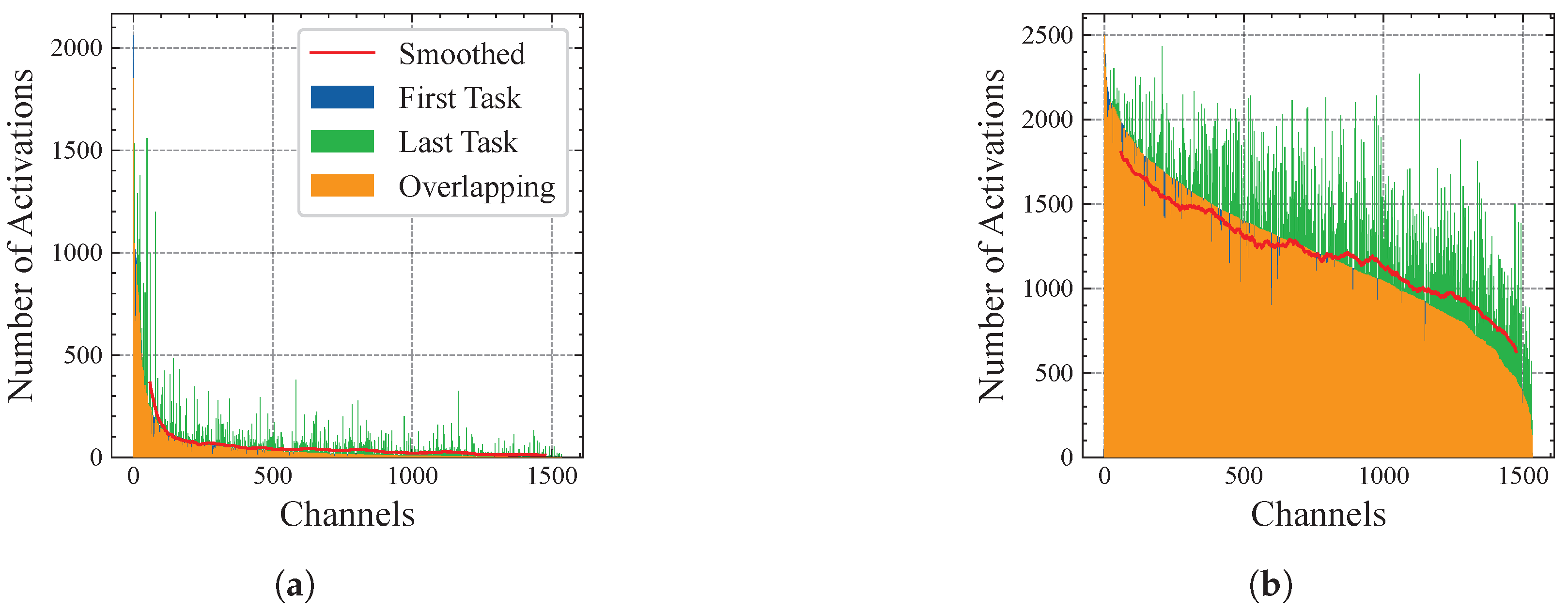
• We conduct detailed analysis on feature channel activation and examine the advantages of the FeTT model in alleviating excessive suppression.
• Extensive benchmark experiments and ablation studies validate the superior performance of the proposed model.

2. Related Work

2.1. Class-Incremental Learning

Generally, there are four directions [12,32,33] of CIL methods: regularization, memory replay, dynamic-architecture-based, and pre-trained methods. Regularization-based methods typically impose constraints between new and old models to alleviate forgetting during training, such as constraints on importance weights [18,19] and knowledge distillation (KD) [20,21]. Memory replay methods [8,22] usually weaken the strict CIL settings by maintaining a small subset data from previous tasks, or synthesizing virtual data [34,35] using generative models. Later, some works further combine the replay with distillation regularization to yield more performance improvements [23,36]. Dynamic-architecture-based methods [24,25,26] primarily freeze the models trained on previous tasks to mitigate forgetting, while allocating additional parameter space to learn new tasks. Due to the excellent feature representations provided by pre-trained models (PTMs) [37,38], recent methods have also gradually benefited from the performance enhancement brought by PTMs, including prompt tuning [27,28,29], zero-shot learning [39,40], and prototype classification [30,41,42].

As mentioned above, PTM-based methods have shown more promising capabilities. However, the prompt tuning strategy [27] usually necessitates learnable parameters at each task stage, resulting not only in additional parameter overhead but also posing potential risks of forgetting due to continual training with mismatched data distributions. Zero-shot learning [39,40] typically incurs significant costs in terms of acquiring large text-image training datasets. As for prototype methods, there is a requirement to retain additional random matrices [42] and a class covariance matrix [41]. On the contrary, our proposed method directly transforms feature representations without requiring any additional parameters or training costs. Moreover, this paper also elucidates the trade-off between stability and plasticity within PTM-based methods from a data distribution perspective.

2.2. Pre-Trained Models (PTMs) and Fine-Tuning

The pre-training paradigm in natural language processing (NLP) [43,44] is gradually being transferred to computer vision (CV) [38,45], enabling deep neural network models to exhibit exceptional capabilities in image feature representation, such as supervised pre-training [46,47], self-supervised pre-training [45,48], and vision-language contrastive pre-training [38,49]. As discussed in Section 2.1, the outstanding feature representation capability of PTMs has greatly enhanced performance in CIL scenarios.

The gap between PTMs and downstream tasks generally necessitates fine-tuning procedures. Early conventional transfer learning methods involved directly fine-tuning all model parameters [50], which inevitably required numerous training iterations and substantial datasets. Then, the introduction of parameter-efficient fine-tuning (PEFT) strategies, such as VPT [51], LoRA [52], SSF [53], and Adapter [54], significantly reduces the expense of fine-tuning overhead, leading to broad application prospects. Following the previous setup [30], this paper extensively applies the proposed method in a plug-and-play manner to various PEFT strategies for comprehensive comparison.

2.3. Feature Transformation

Feature transformation mainly consists of two categories: parametric transformations that involve learnable parameters and non-parametric (training-free) transformations. Broadly speaking, for the former, deep models, including MLPs, attention mechanisms [3], normalization [55], and even the PEFT methods mentioned above [51,53], can all be regarded as transformation operations on features to obtain better latent representations. However, it is evident that achieving a good transformation typically requires training data and an optimization process. On the other hand, training-free transformations directly refine features without requiring any additional parameters or training overhead, mainly including non-linear functions [56,57], chain-of-thought mechanisms [58], and FFT scale functions [59]. In this paper, we propose incorporating training-free transformations onto the backbone model. This approach eliminates the need for parameter updates in CIL, thereby mitigating catastrophic forgetting caused by the unavailability of old task data. By leveraging non-parametric transformations to adapt to all tasks and improve the plasticity, we enable a superior feature space for discrimination in CIL scenarios.

3. Method

3.1. Preliminaries

3.1.1. Problem Formulation

In CIL settings [8], the training data distribution $P_{{\mathcal{D}}_t}$ at each incremental task t is composed of $N_t$ sample pairs without any previous memory instances, denoted by ${\left\{({\mathbf{x}}_{t,i},y_{t,i})\right\}}_{i=1}^{N_t}$, where ${\mathbf{x}}_{t,i}$ and $y_{t,i}$ are the i-th sample pair at the t-th task from data and target space ${\mathcal{X}}_t$ and ${\mathcal{Y}}_t$, respectively. Note that the target spaces at different tasks are assumed to be non-overlapping, i.e., ${\mathcal{Y}}_i\cap {\mathcal{Y}}_j=\varnothing$ for $i\ne j$. For the model F parameterized by $\theta$, our objective is to learn on a current task dataset $P_{{\mathcal{D}}_t}$ and retain classification ability across all previously learned tasks $P_{{\mathcal{D}}_{1:t}}$.

3.1.2. Parameter-Efficient Fine-Tuning (PEFT)

In this section, we briefly elaborate on the employed PEFT methods [30], including VPT [51], SSF [53], and Adapter [54].

Visual Prompt Tuning (VPT) [51] prepends a small amount of learnable parameters tokens to each transformer blocks’ input space. Formally, at i-th block layer $L_i$, given patch embeddings ${\mathbf{E}}_{i-1}$ and the class tokens ${\mathbf{x}}_{i-1}^{\mathrm{cls}}$, the learnable prompt tokens ${\mathbf{P}}_{i-1}$ are added for attention interaction,

$$\begin{array}{cc}\hfill \left[{\mathbf{x}}_i^{\mathrm{cls}},\_,{\mathbf{E}}_i\right]& =L_i\left(\left[{\mathbf{x}}_{i-1}^{\mathrm{cls}},{\mathbf{P}}_{i-1},{\mathbf{E}}_{i-1}\right]\right).\hfill \end{array}$$

(1)

Scale and Shift (SSF) [53] performs the scaling and shifting transformation to modulate the intermediate features. Specifically, given the input features ${\mathbf{x}}_{\mathrm{in}}^{\mathrm{feat}}$, and the scale, shift factors $\gamma$, $\beta$, the output ${\mathbf{x}}_{\mathrm{out}}^{\mathrm{feat}}$ is calculated as,

$${\mathbf{x}}_{\mathrm{out}}^{\mathrm{feat}}=\gamma \otimes {\mathbf{x}}_{\mathrm{in}}^{\mathrm{feat}}+\beta .$$

(2)

Adapter [54] is typically integrated additively into attention blocks via a bottleneck mechanism, which includes learnable weights for upsampling and downsampling. Assuming ${\mathbf{x}}_{\ell }^{\mathrm{feat}}$ is the feature at ℓ-th attention block, we have the following tuning process to obtain the output ${\mathbf{x}}_{\ell }^{\prime \mathrm{feat}}$:

$${\mathbf{x}}_{\ell }^{\prime \mathrm{feat}}=\mathrm{FFN}\left({\mathbf{x}}_{\ell }^{\mathrm{feat}}\right)+s·\mathrm{ReLU}\left({\mathbf{x}}_{\ell }^{\mathrm{feat}}·{\mathbf{W}}_{\mathrm{down}}\right)·{\mathbf{W}}_{\mathrm{up}},$$

(3)

where s is a scale value and ${\mathbf{W}}_{\mathrm{down}}$ and ${\mathbf{W}}_{\mathrm{up}}$ represent the learnable weight parameters for downsampling and upsampling operations in Adapter, respectively.

3.2. PTM-Based CIL for Stability and Plasticity

Following the notations in Section 3.1.1, when conducting supervised training with dataset, our aim is to find the function within the hypothesis space $F\in \mathcal{F}$ that minimizes the expected risk error $\overline{\mathcal{R}}\left(F\right)={\mathbb{E}}_{{\overline{P}}_{\mathcal{D}}}\left[\ell \left(F\right(\mathbf{x}),y)\right]$. Based on the good approximation of the population distribution ${\overline{P}}_{\mathcal{D}}$ by the empirical distribution $P_{\mathcal{D}}$, the empirical risk minimization (ERM) [60] suggests to minimize the risk on empirical data distribution to approximate the expected risk $\mathcal{R}\left(F\right)={\mathbb{E}}_{(\mathbf{x},y)\sim P_{\mathcal{D}}}\left[\ell \left(F\right(\mathbf{x}),y)\right]$. To summarize, a model derived from ERM is considered effective only when the distribution of the training data closely approximate the ideal distribution (test distribution).

From the data distribution perspective, CIL training distributions can be modeled by mixing uniform distribution [23] with the number of sample instances. Formally, given the empirical data distribution $P_{{\mathcal{D}}_t}(\mathbf{x},y)$ at task t, we extend the vanilla model framework to exemplar-free setting, and the class marginal distribution $P_{{\mathcal{D}}_t}\left(y\right)$ is formalized as follows:

$$P_{{\mathcal{D}}_t}\left(y\right)=\int P_{{\mathcal{D}}_t}(\mathbf{x},y)\mathrm{d}\mathbf{x}=\mathbf{U}\left(\right|{\mathcal{Y}}_{1:t-1}|,|{\mathcal{Y}}_{1:t}\left|\right),$$

(4)

where $\mathbf{U}$ denotes the uniform distribution and $|{\mathcal{Y}}_{1:t-1}|$ and $|{\mathcal{Y}}_{1:t}|$ denote the number of classes in previous tasks and all classes at t-th task, respectively. However, in CIL scenarios, the ideal population distribution or test distribution is uniformly distributed across all categories $P_{{\mathcal{D}}_t}^{\mathrm{test}}\left(y\right)=\mathbf{U}(0,|{\mathcal{Y}}_{1:t}\left|\right)$.

3.2.1. Plasticity CIL Method

Plasticity-oriented PTM-based CIL methods [27,28] aim to fine-tune training for each task t to acquire novel knowledge based on the current training data distribution $P_{{\mathcal{D}}_t}$. Given data pairs $(\mathbf{x},y)\sim P_{{\mathcal{D}}_t}$ and pre-trained model F parameterized by $\theta$,

$$arg\underset{\varphi }{min}{\mathbb{E}}_{(\mathbf{x},y)\sim P_{{\mathcal{D}}_t}}\left[\ell \left(F_{\theta ,\varphi }\left(\mathbf{x}\right),y\right)\right],$$

(5)

where $\varphi$ denotes the additional trainable parameters with PEFT strategies, aiming to achieve the optimal ${\varphi }^{*}$ by minimizing the objective loss function ℓ. Obviously, there exists a significant disparity between the training and test data distribution, i.e., $P_{{\mathcal{D}}_t}\left(y\right)$ and $P_{{\mathcal{D}}_t}^{\mathrm{test}}\left(y\right)$ when $t>1$, as shown in Figure 1b. Despite the fact that the PEFT strategy facilitates the model in tuning just a few extra parameters and preserving the original feature space, the optimization of the data distribution remains confined to the new task ${\mathcal{Y}}_t$, consequently overlooking the previous tasks ${\mathcal{Y}}_{1:t-1}$.

3.2.2. Stability CIL Method

In the first task, since no extra incremental tasks have been performed, the data distribution remains temporarily matched, i.e., $P_{{\mathcal{D}}_1}\left(y\right)=P_{{\mathcal{D}}_1}^{\mathrm{test}}\left(y\right)$. Stability-oriented PTM-based CIL methods [30] employ PEFT on such training distribution to adapt on downstream task data.

$$arg\underset{\varphi }{min}{\mathbb{E}}_{(\mathbf{x},y)\sim P_{{\mathcal{D}}_1}}\left[\ell \left(F_{\theta ,\varphi }\left(\mathbf{x}\right),y\right)\right].$$

(6)

Then, the fine-tuned backbone model is frozen to avoid training distributional discrepancies, i.e., $P_{{\mathcal{D}}_{t(t>1)}}\left(y\right)\ne P_{{\mathcal{D}}_{t(t>1)}}^{\mathrm{test}}\left(y\right)$, as shown in Figure 1c. However, despite retaining the acquired knowledge and even the PTMs feature representation space, the model exhibits an insufficient acquisition of knowledge on new tasks ${\mathcal{Y}}_{t(t>1)}$.

In summary, to the best of our knowledge, this is the first discussion on PTM-based CIL methods from the perspective of training and test distributions. The plasticity-oriented and stability-oriented PTM-based CIL methods focus on different aspects of the trade-off between the stability and plasticity. Therefore, the FeTT model is proposed to address the above limitations for learning novel classes incrementally: freezing the model in subsequent incremental tasks to maintain stability while performing training-free feature transformation to enhance plasticity.

3.3. Feature Transformation Tuning Model

The overall architecture of our proposed FeTT model is shown in Figure 2, and the pseudocode is presented in Algorithm 1. In the first task, since there are no missing data, and the training and test data share a consistent class marginal distribution, we perform PEFT to boost the performance of the first task while narrowing the data domain gap for future arriving categories. For the following incremental tasks, the discrepancy in data distribution leads us to directly freeze the model and only update the class prototypes for classification. We additionally employ the feature transformation on the backbone features of all tasks to regulate the feature channel activations. Further empirical discussion and analysis of our proposed FeTT model are elaborated in Section 3.4.

Formally, according to the notation in Section 3.1.1 and Section 3.2.2, given training data pairs $(\mathbf{x},y)\sim P_{{\mathcal{D}}_1}$ in the first task, a pre-trained model F parameterized by $\theta$, and additional PEFT trainable parameters $\varphi$, we optimize Equation (7) to achieve the optimal ${\varphi }^{*}$ by minimizing the cross-entropy objective loss function ℓ.

$$\begin{array}{c}\hfill F_{\theta ,{\varphi }^{*}}=arg\underset{\varphi }{min}{\mathbb{E}}_{(\mathbf{x},y)\sim P_{{\mathcal{D}}_1}}\left[\ell \left(F_{\theta ,\varphi }\left(\mathbf{x}\right),y\right)\right].\end{array}$$

(7)

Then, the cosine similarity metric $\cos (·,·)$ based loss function is defined as follows,

$$\ell (F_{\theta ,\varphi }\left(\mathbf{x}\right),y)=\ell (\mathbf{z},y)=-\sum _{i=1}^C{y}_{i}log{\displaystyle \frac{e^{cos(\mathbf{z},{\mathbf{w}}_y)}}{{\sum }_j{e}^{cos(\mathbf{z},{\mathbf{w}}_j)}}},$$

(8)

where $\mathbf{z}=F_{\theta ,\varphi }\left(\mathbf{x}\right)$ denotes the backbone feature embeddings, the total number of classes is C, and $\mathbf{W}={\mathbf{w}}_{1:C}$ denotes the weight of the classifier. The objective loss function, as formulated in Equation (8), drives the model to minimize empirical risk error only on current training data ${\mathcal{D}}_t$, while disregarding previous data distributions ${\mathcal{D}}_{1:t-1}$. This oversight may fundamentally explain the catastrophic forgetting phenomenon in continual learning systems from the perspective of data distribution. Therefore, as in Equation (7), our model adopts a similar formulation in the stability CIL method. Equation (6) only achieves adaptive fine-tuning of the model on the first task, effectively avoiding severe knowledge degradation of previous tasks during continual fine-tuning. Then, the fine-tuned model $F_{\theta ,{\varphi }^{*}}$ is frozen and concatenated with the original PTM $F_{\theta }$ to retain both adaptability to downstream tasks and the original generalization capability [30].

$$\mathbf{z}\prime =F_{\theta ,{\varphi }^{*}}^{\prime }\left(\mathbf{x}\right)=[F_{\theta ,{\varphi }^{*}}\left(\mathbf{x}\right),F_{\theta }\left(\mathbf{x}\right)],$$

(9)

where $[,]$ denotes the concatenate operation.

Next, we introduce two element-wise transformation functions $T\left(x\right)$ [56,57,61] to refine the features $\mathbf{z}$.

$$\mathrm{LogTrans}\left(x\right)=T\left(x\right)={\displaystyle \frac{1}{{ln}^{\eta }\left(\frac{1}{x}+1\right)}},$$

(10)

$$\mathrm{PwrTrans}\left(x\right)=T\left(x\right)=x^{\kappa },$$

(11)

where $\eta$ and $\kappa$ are two hyper-parameters. The feature transformation is non-parametric in nature, as it modifies the channel activations [62,63] directly to suit both previous old and new tasks, without considering the impact of discrepancy in data distributions, leading to performance and plasticity improvements. When combined with the PEFT strategy in Equation (7), the fusion of parametric PEFT and non-parametric transformation results in further significant performance gains.

Algorithm 1 FeTT model

Require: Backbone parameters $\theta$, PEFT parameters $\varphi$, CIL tasks T, Dataset $P_{{\mathcal{D}}_t}$ at task t. for task $t=1,2,\dots ,T$ do      if task $t=1$ then         Train $\varphi$ by minimizing the error on $P_{{\mathcal{D}}_1}$ in Equation (7);      end if      Forward $\theta$ and $\varphi$ based on dataset $P_{{\mathcal{D}}_t}$ in Equation (9);      Perform feature transformation tuning in Equation (12);      Update category prototypes in Equation (13) for classifier. end for

In practice, these two functions serve similar effects, and we directly employ the former function in the FeTT model, while for optional ensemble strategies, we apply the two different transformations to the models separately. Then, we obtain the FeTT feature embeddings:

$$\mathbf{z}\prime \prime =\mathrm{LogTrans}(\mathbf{z}\prime ),\mathrm{or}\mathbf{z}\prime \prime =\mathrm{PwrTrans}(\mathbf{z}\prime ).$$

(12)

Finally, in each task, update the class prototype by averaging all FeTT features of the same category as the classifier weights.

$${\mathbf{w}}_y={\displaystyle \frac{1}{N_y}}\sum _{i=1}^{N_y}{\mathbf{z}}_y^{\prime \prime },$$

(13)

where ${\mathbf{z}}_y^{\prime \prime }$ and $N_y$ denote the FeTT features and number of samples in class y, respectively. During the evaluation, we perform the classification using cosine similarity.

$$p_y={\displaystyle \frac{e^{cos(\mathbf{z}\prime \prime ,{\mathbf{w}}_y)}}{{\sum }_j{e}^{cos(\mathbf{z}\prime \prime ,{\mathbf{w}}_j)}}}.$$

(14)

Additionally, we extend the model to the optional ensemble strategy for FeTT-E, combining scores from two distinct PTMs for classification.

$$p_y={\displaystyle \frac{e^{cos({\mathbf{z}}_0^{\prime \prime },{\mathbf{w}}_y)+cos({\mathbf{z}}_1^{\prime \prime },{\mathbf{w}}_y)}}{{\sum }_j{e}^{cos({\mathbf{z}}_0^{\prime \prime },{\mathbf{w}}_j)+cos({\mathbf{z}}_1^{\prime \prime },{\mathbf{w}}_j)}}},$$

(15)

where ${\mathbf{z}}_0^{\prime \prime }$ and ${\mathbf{z}}_1^{\prime \prime }$ are FeTT features from different two PTMs. Various PTMs exhibit unique inductive biases toward downstream tasks. The optional introduction of diverse models is intended to broaden the feature space of PTMs. Note that in experimental comparisons, we ensure fairness by presenting results from the same single PTM for comparison.

3.4. Feature Channel Activations

In this section, we further analyze the effect of the FeTT model from the perspective of feature channel activations. Inspired by activation frequency patterns [63], we extend our analysis to examine the feature channel activations in different CIL tasks. Specifically, based on the sample feature embeddings of the first and last tasks in the CIFAR100 B0 Inc5 benchmark, a channel is deemed activated if its activation value exceeds a certain threshold (e.g., 10% of the maximum activation value over all channels). Subsequently, we calculate the activation frequency of each channel for both the first and the final tasks, respectively. Finally, we produce the histogram by organizing the feature channels in descending order according to the activation frequency of the first task, as shown in Figure 3.

As shown in Figure 3a, for the first task activations of the baseline model, owing to the PEFT on the first task data, the model exhibits a high activation frequency to channels associated with the first task categories, while other unrelated channels are suppressed. Intuitively, different feature channels exhibit distinct responses to different categories [62]; therefore, in the CIL scenario, there should naturally be differences in the channel activation patterns between newly arrived categories and the existing categories. However, the activation frequency for the last task exhibits a similar frequency to that of the first task data. Channels that potentially hold discriminative power for future classification appear to be suppressed.

As for our FeTT model, firstly, we can observe that the transformation function $T\left(x\right)$ in Equations (10) and (11) exhibits similar property [57]: when $x>0$, then $T^{\prime }\left(x\right)>0$, $T^{\prime \prime }\left(x\right)<0$, and ${lim}_{x\to 0^{+}}{T}^{\prime }\left(x\right)=+\infty$. The first-order derivative indicates that the relative relationship of the features remains unchanged. Then, applying the same transformation to all CIL tasks ensures the consistency of previous knowledge, preserving the fundamental discriminative nature of the backbone features. Meanwhile, the channel value close to zero are greatly amplified to enhance the response of suppressed features, preparing in advance for newly arriving classes. Additionally, the second derivative indicates a further reduction in the response differences between feature channels, alleviating the issue of certain feature channels dominating and suppressing others. As shown in Figure 3b, compared with the baseline model, our results indicate that the FeTT model exhibits activations of a wider range of channels on both the first task and last task. Moreover, compared with overlapping, the moving average curve suggests that the activation for the last task decreases in the head channels while it increases in the tail channels. This observation identifies not only a mitigation of inhibition, but also indicates a reduction in the dependency of the last task on the highly activated head channels of the first task.

4. Experimental Results

4.1. Setups

4.1.1. Datasets

According to the CIL benchmark settings [28,30,64], this paper conducts experiments on six datasets, including CIFAR100 [65], CUB200 [66], ImageNet-A (IN-A) [67], ImageNet-R (IN-R) [68], ObjectNet (Obj) [69], and VTAB [70].

CIFAR100 [65] is a dataset of $32\times 32$ RGB images, comprising a total of 100 classes and 60,000 images, where 50,000 are used for training and 10,000 for testing. CUB200 [66] is a dataset for fine-grained bird species visual classification tasks, consisting of a total of 200 categories. ImageNet-R [68] and ImageNet-A [67] can be considered as two 200-class datasets evolved from the standard ImageNet [71] dataset, where the former incorporates various artistic renditions, while the latter focuses on natural adversarial examples. ObjectNet [69] consists of a total of 313 categories, with objects in the collected images appearing in cluttered natural scenes and exhibiting unusual poses. In this paper, we follow the settings in [30] and select subset of 200 classes for CIL scenario. VTAB [70] was originally designed as a cross-domain evaluation benchmark, comprising a total of 19 datasets divided into 3 groups: natural, specialized, and structured. Following the setup described in [30], we select five datasets from these groups to create a task for cross-domain class-incremental learning.

4.1.2. Benchmarks

Currently, the evaluation benchmark protocols for CIL mainly consist of two aspects [8,24]. On the one hand, the dataset is partitioned directly into incremental tasks, where all categories are uniformly divided. On the other hand, the model first learns half of the categories (base categories) in the dataset, followed by incremental learning on the remaining half of the categories. The aforementioned protocols are denoted as the Base 0/Half, incremental n task (abbreviated as B 0/H Inc n), with n representing the number of classes learned per incremental task. The Base 0 and Base Half, respectively, denote conducting incremental tasks directly and learning half of the classes in the first incremental task. We build a comprehensive and detailed comparison benchmark that includes a total of 14 different settings.

4.1.3. Evaluation Metrics

The metrics used in this paper are all based on the top-1 classification accuracy. Specifically, we report the average accuracy $\overline{\mathcal{A}}={\displaystyle \frac{1}{T}}{\sum }_{t=1}^T{\mathcal{A}}_t$ across all tasks as the main quantitative metric for all settings, where ${\mathcal{A}}_t$ denotes the accuracy on all previously learned tasks after the t-th task and T denotes the total number of tasks. Additionally, the last accuracy ${\mathcal{A}}_T$ after completing all incremental tasks is also considered for comprehensive evaluation.

4.2. Implementation Details

We implement all our model with PyTorch [72]. During model parameter-efficient fine-tuning (PEFT) in the first task, we employ the SGD optimizer with a weight decay of 5e-4 across all datasets. The learning rate is set to 0.01 and a cosine annealing schedule is employed. Additionally, the total number of epochs is set to 20, with a batch size of 48. The standard data pre-processing procedures, such as random crop and horizontal flip, are employed to ensure that the input images are scaled to $224\times 224$ dimensions. For pre-trained models (PTMs), we follow the same benchmark settings as before [30], using the ImageNet-21k pre-trained Vision Transformer (ViT-B/16) as the feature extractor backbone. When employing optional ensemble strategies, another model utilizes ImageNet-1k based pre-trained ViT to enhance ensemble diversity. The category order of all incremental tasks remains consistent with previous work [30]. The hyper-parameters $\eta$ and $\kappa$ of our proposed transformation tuning are mainly set to $0.1$ and $0.3$, respectively.

4.3. Main Results

Our proposed method is compared with various models, including fine-tuning, LwF [21], L2P [27], DualPrompt [28], CODA-Prompt [29], SimpleCIL, and ADAM [30]. We further divide the above methods into two categories according to Section 3.2: stability (S.) and plasticity (P.). In addition, we conduct detailed comparisons by seamlessly integrating the FeTT model and optional ensemble FeTT-E model into various PEFT strategies in a plug-and-play manner. The numerical results of the comparative methods are cited from [30]. For the ADAM model [30], the results are reported based on the selection of the best outcome as indicated in the original paper. For the methods marked with †, the results are based on our re-implementation using open-source code. Note that all the results use the same ImageNet-21k pre-trained ViT-B/16 model, except ours, i.e., FeTT-E, uses both ImageNet-21k and ImageNet-1k models for ensemble strategy.

Table 1. Comparison results of average accuracy $\overline{\mathcal{A}}$ and last accuracy ${\mathcal{A}}_T$ on six datasets. Note that IN-R, IN-A, and Obj denote the abbreviations of ImageNet-R, ImageNet-A, and ObjectNet datasets, respectively. $\Delta$ and gray boxes highlight the performance gap. * indicates the best results cited from the original paper. † denotes the re-implemented results using open source code. P. and S. denote plasticity and stability, respectively, as described in Section 3.2.

Method		CIFAR B0 Inc5		CUB B0 Inc10		IN-R B0 Inc5		IN-A B0 Inc10		Obj B0 Inc10		VTAB B0 Inc10
		$\overline{\mathcal{A}}$	${\mathcal{A}}_{\mathbf{T}}$	$\overline{\mathcal{A}}$	${\mathcal{A}}_{\mathbf{T}}$	$\overline{\mathcal{A}}$	${\mathcal{A}}_{\mathbf{T}}$	$\overline{\mathcal{A}}$	${\mathcal{A}}_{\mathbf{T}}$	$\overline{\mathcal{A}}$	${\mathcal{A}}_{\mathbf{T}}$	$\overline{\mathcal{A}}$	${\mathcal{A}}_{\mathbf{T}}$
P.	Fine-Tuning	$38.90$	$20.17$	$26.08$	$13.96$	$21.61$	$10.79$	$21.60$	$10.96$	$19.14$	$8.73$	$34.95$	$21.25$
	Fine-Tuning Adapter	$60.51$	$49.32$	$66.84$	$52.99$	$47.59$	$40.28$	$43.05$	$37.66$	$50.22$	$35.95$	$48.91$	$45.12$
	LwF [21]	$46.29$	$41.07$	$48.97$	$32.03$	$39.93$	$26.47$	$35.39$	$23.83$	$33.01$	$20.65$	$40.48$	$27.54$
	L2P [27]	$85.94$	$79.93$	$67.05$	$56.25$	$66.53$	$59.22$	$47.16$	$38.48$	$63.78$	$52.19$	$77.11$	$77.10$
	DualPrompt [28]	$87.87$	$81.15$	$77.47$	$66.54$	$63.31$	$55.22$	$52.56$	$42.68$	$59.27$	$49.33$	$83.36$	$81.23$
	CODA-Prompt [29]	$89.11$	$81.96$	$84.00$	$73.37$	$64.42$	$55.08$	$48.51$	$36.47$	$66.07$	$53.29$	$83.90$	$83.02$
S.	SimpleCIL [30]	$87.57$	$81.26$	$92.20$	$86.73$	$62.58$	$54.55$	$60.50$	$49.44$	$65.45$	$53.59$	$85.99$	$84.38$
	ADAM * [30]	$90.65$	$85.15$	$92.21$	$86.73$	$72.35$	$64.33$	$62.81$	$51.48$	$69.15$	$56.64$	$87.47$	$85.36$
Ours	SimpleCIL†	$87.57$	$81.26$	$92.23$	$86.77$	$62.39$	$54.33$	$60.63$	$48.45$	$65.45$	$53.59$	$86.34$	$84.46$
	+ FeTT	$89.22$	$83.42$	$92.41$	$87.02$	$64.32$	$56.55$	$63.58$	$52.34$	$67.13$	$54.68$	$88.83$	$87.61$
	$\Delta$	$+1.65$	$+2.16$	$+0.18$	$+0.25$	$+1.93$	$+2.22$	$+2.95$	$+3.89$	$+1.68$	$+1.09$	$+2.49$	$+3.15$
	+ FeTT-E	$88.81$	$83.12$	$92.08$	$86.94$	$68.66$	$61.97$	$65.93$	$54.71$	$67.20$	$55.05$	$88.97$	$87.82$
	$\Delta$	$+1.24$	$+1.86$	$-0.15$	+0.17	$+6.27$	$+7.64$	+5.30	$+6.26$	$+1.75$	+1.46	$+2.63$	$+3.36$
	ADAM (VPT) †	$85.28$	$78.24$	$91.79$	$85.92$	$55.75$	$47.08$	$48.62$	$37.39$	$62.03$	$49.17$	$82.18$	$79.94$
	+ FeTT	$88.00$	$82.40$	$91.80$	$85.96$	$65.79$	$57.62$	$57.85$	$46.15$	$67.24$	$54.60$	$85.86$	$83.65$
	$\Delta$	$+2.72$	$+4.16$	$+0.01$	$+0.04$	$+10.04$	$+10.54$	$+9.23$	$+8.76$	$+5.21$	$+5.43$	$+3.68$	$+3.71$
	+ FeTT-E	$88.58$	$82.84$	$91.73$	$86.22$	$68.95$	$61.12$	$55.37$	$44.04$	$68.22$	$55.76$	$86.63$	$85.10$
	$\Delta$	$+3.30$	$+4.60$	$-0.06$	+0.30	$+13.20$	$+14.04$	$+6.75$	$+6.65$	$+6.19$	$+6.59$	$+4.45$	$+5.16$
	ADAM (SSF) †	$87.89$	$81.88$	$91.80$	$86.43$	$68.99$	$60.63$	$61.04$	$49.11$	$69.12$	$56.38$	$86.31$	$82.55$
	+ FeTT	$89.05$	$83.67$	$91.81$	$86.43$	$73.65$	$66.10$	$64.03$	$52.47$	$70.14$	$57.30$	$89.50$	$87.64$
	$\Delta$	$+1.16$	$+1.79$	$+0.01$	$+0.00$	$+4.66$	$+5.47$	$+2.99$	$+3.36$	$+1.02$	$+0.92$	$+3.19$	$+5.09$
	+ FeTT-E	$88.94$	$83.74$	$91.69$	$86.64$	$75.32$	$68.00$	$67.31$	$55.04$	$69.91$	$57.09$	$90.27$	$88.46$
	$\Delta$	$+1.05$	$+1.86$	$-0.11$	+0.21	$+6.33$	$+7.37$	$+6.27$	$+5.93$	$+0.79$	$+0.71$	$+3.96$	$+5.91$
	ADAM (Adapter) †	$90.58$	$85.04$	$92.24$	$86.73$	$62.85$	$54.78$	$60.78$	$48.65$	$67.15$	$55.21$	$86.24$	$84.38$
	+ FeTT	$91.78$	$86.76$	$92.32$	$86.94$	$64.78$	$57.15$	$63.53$	$52.21$	$69.05$	$56.83$	$88.82$	$87.63$
	$\Delta$	$+1.20$	$+1.72$	$+0.08$	$+0.21$	$+1.93$	$+2.37$	$+2.75$	$+3.56$	$+1.90$	$+1.62$	$+2.58$	$+3.25$
	+ FeTT-E	$91.96$	$86.94$	$92.07$	$86.94$	$69.04$	$62.38$	$65.90$	$54.64$	$69.46$	$57.26$	$88.97$	$87.82$
	$\Delta$	$+1.38$	$+1.90$	$-0.17$	$+0.21$	$+6.19$	$+7.60$	$+5.12$	$+5.99$	$+2.31$	$+2.05$	$+2.73$	$+3.44$

and Figure 4 summarize the main quantitative results of various methods on different datasets. Overall, with the support of our proposed model, whether employing the SimpleCIL method of classifying prototypes using frozen PTMs or different PEFT-based ADAM strategies, we can observe a noticeable improvement in both average and last accuracy performance, validating the effectiveness of our proposed model. Furthermore, the accuracy line plots for each task in Figure 4 demonstrate that our method mainly outperforms other methods, indicating strong performance improvements across all task stages. In particular, on the CIFAR B0 Inc5 benchmark, employing our FeTT method with SimpleCIL by prototype classification leads to the enhancement from $87.57\%$ to $89.22\%$ ($+1.65\%$) and $81.26\%$ to $83.42\%$ ($+2.16\%$) on average and last accuracy, respectively. With the Adapter PEFT strategy, our FeTT-E model demonstrate the improvement in the average and last accuracy from $90.58\%$ to $91.96\%$ ($+1.38\%$) and $85.04\%$ to $86.94\%$ ($+1.90\%$). Additionally, on cross-domain CIL VTAB benchmark, we achieve performance with an average and last accuracy of $90.27\%$ and $88.46\%$ based on the SSF PEFT strategy. In summary, our proposed method improves performance and confirms its plug-and-play versatility across different dataset scenarios. It should be noted that, compared to FeTT, the performance does not always increase with FeTT-E ensemble. Specifically, FeTT-E model primarily demonstrates further performance on the ImageNet-R, ImageNet-A, and VTAB datasets, yet it does not consistently yield performance gains across all datasets like CIFAR and CUB. We believe that this could be attributed to the inductive biases of different PTMs when dealing with downstream task data. The dataset variation between ImageNet-1k and ImageNet-21k could potentially result in performance differences. For larger domain gaps and fine-grained image datasets like CIFAR and CUB datasets, the ImageNet-21k based PTMs may be more suitable. Moreover, for the fine-grained CUB benchmark depicted in Figure 4, the performance levels have consistently remained high, having reached a saturation point. The comparative efficacy of different methods is close, demonstrating a trend of diminishing marginal returns. We also directly use the FeTT model for inference due to the matching of pre-trained knowledge and performance improvement. Conversely, for downstream tasks derived from standard ImageNet dataset such as ImageNet-A and ImageNet-R, the ImageNet-1k based PTMs might exhibit superior performance. Still, FeTT-E is equally outstanding and competitive with the baseline models.

4.4. Ablation Study

In this section, we conduct comprehensive ablation studies to validate the effectiveness of our proposed method.

As shown in

Table 2. Ablation results of average accuracy $\overline{\mathcal{A}}$ and last accuracy ${\mathcal{A}}_T$ on ObjectNet and ImageNet-A datasets. Log and Pwr are the Log transformation and Power transformation, respectively. Ens. is the abbreviation for ensemble strategy. ✓ indicates the use of the corresponding component. The best results are in bold.

Baseline	Ablations			Obj		IN-A
	Log	Pwr	Ens.	$\overline{\mathcal{A}}$	${\mathcal{A}}_{\mathit{T}}$	$\overline{\mathcal{A}}$	${\mathcal{A}}_{\mathit{T}}$
SimpleCIL				$65.45$	$53.59$	$60.63$	$48.45$
	✓			$67.13$	$54.68$	$63.58$	$52.34$
		✓		$66.99$	$54.66$	$63.54$	$52.34$
			✓	$65.69$	$53.74$	$61.79$	$51.15$
	✓	✓	✓	$\mathbf{67}.\mathbf{21}$	$\mathbf{55}.\mathbf{05}$	$\mathbf{65}.\mathbf{93}$	$\mathbf{54}.\mathbf{71}$
ADAM (Adapter)				$67.15$	$55.21$	$60.78$	$48.65$
	✓			$69.05$	$56.83$	$63.53$	$52.21$
		✓		$68.96$	$56.76$	$63.52$	$52.21$
			✓	$68.00$	$56.26$	$61.74$	$51.02$
	✓	✓	✓	$\mathbf{69}.\mathbf{46}$	$\mathbf{57}.\mathbf{26}$	$\mathbf{65}.\mathbf{90}$	$\mathbf{54}.\mathbf{64}$

, the ablation experiments are performed on the baseline model of SimpleCIL and of the Adapter-based PEFT strategy, respectively, to comprehensively validate the model’s capabilities. The overall benchmark datasets for model ablation includes the ObjectNet and ImageNet-A datasets. Our proposed method mainly consists of two feature transformation functions and an ensemble strategy, resulting in a total of three components.

Clearly, under the baselines of SimpleCIL and Adapter, we can observe performance improvements brought about by applying two transformation functions. Specifically, the Log feature transformation function yields average accuracies of $67.13\%$ and $63.58\%$ on the ObjectNet and ImageNet-A datasets, while the Pwr function achieves average accuracies of $66.99\%$ and $63.54\%$. Compared to the baseline model’s average accuracies of $65.45\%$ and $60.63\%$, both functions show notable performance enhancements, affirming the efficacy of the feature transformation module. When using the Adapter baseline on the ObjectNet dataset, we can observe that, compared to the SimpleCIL baseline model, the model’s domain gap narrowed via PEFT, leading to a performance improvement from $65.45\%$ to $67.15\%$. Furthermore, our proposed two-feature transformation functions are able to continue to contribute to performance enhancement. Meanwhile, without employing any feature transformation functions, we introduce diverse pre-trained ImageNet-1k ViT model for ensemble, leading to accuracy boosting compared with two baseline models. Finally, with the support of all constituent components, the model performance achieves the most outstanding results.

4.5. Further Exploration

In this section, we conduct an in-depth investigation of our model, including results from different PTMs, analysis of different PEFT dataset sizes, and t-SNE visualization.

4.5.1. Different PTMs

As shown in

Table 3. Ablation results of average accuracy $\overline{\mathcal{A}}$ using different pre-trained models (PTMs) on CIFAR B0 Inc5 benchmark. IN-1K and IN-21K denote the ImageNet-1K and ImageNet-21K pre-trained ViTs. IN-1K-M and IN-21K-M denote the MIIL-pre-process-based pre-trained ViTs [73]. CLIP denotes the pre-trained vision-language model [38]. The best results are in bold.

Ablations	PTMs
	IN-1K	IN-21K	IN-1K-M	IN-21K-M	CLIP
SimpleCIL	$82.79$	$87.57$	$86.35$	$89.75$	$64.63$
+ LogTrans	$\mathbf{85}.\mathbf{61}$	$\mathbf{89}.\mathbf{22}$	$\mathbf{86}.\mathbf{48}$	$\mathbf{89}.\mathbf{93}$	$\mathbf{64}.\mathbf{66}$

, we explore the application of our feature transformation function across various types of PTMs, including ImageNet based ViT-B/16 PTMs, ImageNet-MIIL-based ViT-B/16 PTMs [73], as well as CLIP-based ViT-B/32 PTMs [38]. Obviously, thanks to the pre-training data refinement, the ImageNet-MIIL-based PTMs achieve better performance. On the contrary, the performance of the CLIP model is likely weakest due to the significant gap between the text-image training dataset and the CIFAR dataset. In this paper, although stronger models generally have the potential to achieve better performance in CIL tasks, we mainly adopt the ImageNet-21k based PTMs for fair comparison and benchmark settings. More importantly, applying our feature transformation function to various PTMs consistently shows performance gains in Table 3, underscoring its broad applicability and generalizability. Meanwhile,

Table 4. Ablation results of average accuracy $\overline{\mathcal{A}}$ using ImageNet-1K and ImageNet-21K pre-trained ViT models on ObjectNet and ImageNet-A benchmarks. The best results are in bold.

Ablations	Obj		IN-A
	IN-1K	IN-21K	IN-1K	IN-21K
SimpleCIL	$63.12$	$65.45$	$60.04$	$60.63$
+ FeTT (Ours)	$65.25$	$67.13$	$65.68$	$63.57$
+ FeTT-E (Ours)	$\mathbf{67}.\mathbf{21}$	$\mathbf{67}.\mathbf{21}$	$\mathbf{65}.\mathbf{93}$	$\mathbf{65}.\mathbf{93}$

further illustrates the experimental results of single models and ensemble models on the ObjectNet and ImageNet-A datasets using IN-1k and IN-21k PTMs. The performance improvement of FeTT-E model over individual models suggests the promising potential of integrating diverse models.

4.5.2. PEFT Dataset Sizes

As for the results of dataset sizes,

Table 5. Ablation results of last accuracy ${\mathcal{A}}_T$ using different parameter-efficient fine-tuning (PEFT) data volumes in the first step (measured by number of classes) on the CIFAR dataset. ‘None’ signifies the absence of any training data, which degrades to the SimpleCIL method. The best results are in bold.

Ablations	Number of Training Classes in First Step for PEFT
	None	2 Classes	5 Classes	10 Classes	20 Classes	40 Classes
ADAM (Adapter)	$81.26$	$81.48$	$85.03$	$87.50$	$88.33$	$89.27$
+ FeTT (Ours)	$\mathbf{83}.\mathbf{42}$	$\mathbf{84}.\mathbf{16}$	$86.75$	$88.76$	$89.39$	$89.93$
+ FeTT-E (Ours)	$83.12$	$83.79$	$\mathbf{86}.\mathbf{96}$	$\mathbf{88}.\mathbf{91}$	$\mathbf{89}.\mathbf{61}$	$\mathbf{90}.\mathbf{17}$

illustrates the impact of different PEFT data volumes in the first task, which are measured by the number of classes. As the volume of data increases gradually, there is a corresponding steady improvement in accuracy. With an ample dataset, PEFT methods can more effectively generalize to new emerging classes, which also substantiates PEFT’s superiority in narrowing the gap between PTMs and downstream task data. On the contrary, in general scenarios where data are limited (e.g., 2 classes of training data), the model obviously tends to suppress feature channels of new classes, as discussed in Section 3.4. Consequently, the accuracy drops to only $81.48\%$, in contrast to an accuracy of $89.27\%$ with 40 classes of data. However, by employing our proposed FeTT model, we achieve an accuracy from $81.48\%$ to $84.16\%$ ($+2.68\%$) with 2 classes of data, validating the effectiveness of performance improvement by mitigating channel suppression. Moreover, when using 40 classes of PEFT first-task data, our model is still capable of achieving further improvements ($89.93\%$ and $90.17\%$ on FeTT and FeTT-E models), proving the effectiveness and generalization of different data sizes.

4.5.3. The t-SNE Visualization

In Figure 5, the t-SNE [74] strategy is employed to visually analyze the feature representations on the CIFAR B0 Inc5 benchmark. Specifically, distinct marker symbols and colors are utilized to symbolize different class samples. Five classes from the first task are marked with circles “∘”, and another five classes in the last incremental task are marked with “×”. In summary, in comparison with the baseline model, our model’s experiential visualization demonstrates superior cohesiveness. Particularly, for the red × markers samples, the baseline model’s samples are scattered into two clusters, separated by black ∘ samples. In contrast, in the results of our proposed FeTT model, the red × markers samples become more compact without a significant intra-class gap.

5. Conclusions

This paper introduces a novel PTM-based class-incremental learning method. We firstly conduct a detailed analysis of the PTM-based CIL methods from the perspective of data distribution, revealing two distinct types, i.e., stability method and plasticity method. Then, we propose the feature transformation tuning (FeTT) model based on these two aspects. Specifically, the PEFT strategy is performed in the first task using matched data distribution to reduce the domain gap between the PTMs and downstream CIL tasks. Subsequently, the model remains frozen for the prototype update to ensure stability while mitigating the mismatch in training data distribution. Additionally, feature transformation is employed to regulate the backbone representations for enhancing model plasticity without incurring any additional training or parameter costs. Extensive experimental results and feature channel activations discussion validate that our proposed model obtains superior performance on CIL benchmarks.

Furthermore, it should be acknowledged that this study has several limitations. On the one hand, we directly propose the use of ImageNet-based PTMs in the CIL scenario for fair comparison. However, utilizing alternative PTMs may yield even more significant performance improvements. Furthermore, the issue of which PTM, e.g., vision-language models (VLMs), is better suited for CIL is still undetermined. On the other hand, our proposed method alleviates the dilemma between the stability and plasticity from the perspective of data distribution. However, the frozen backbone and non-parametric transformations still limit the plasticity of the model’s space. How to perform ERM under mismatched data distributions to effectively conduct CIL remains a research question that has yet to be fully addressed.

References

1. Krizhevsky, A.; Sutskever, I.; Hinton, G.E. ImageNet classification with deep convolutional neural networks. Commun. ACM 2017, 60, 84–90. [Google Scholar]
2. He, K.; Zhang, X.; Ren, S.; Sun, J. Deep Residual Learning for Image Recognition. In Proceedings of the 2016 IEEE Conference on Computer Vision and Pattern Recognition (CVPR 2016), Las Vegas, NV, USA, 27–30 June 2016; IEEE Computer Society: Los Alamitos, CA, USA, 2016; pp. 770–778. [Google Scholar]
3. Vaswani, A.; Shazeer, N.; Parmar, N.; Uszkoreit, J.; Jones, L.; Gomez, A.N.; Kaiser, L.; Polosukhin, I. Attention is All you Need. In Proceedings of the Advances in Neural Information Processing Systems 30 (NeurIPS 2017), Long Beach, CA, USA, 4–9 December 2017; pp. 5998–6008. [Google Scholar]
4. Russakovsky, O.; Deng, J.; Su, H.; Krause, J.; Satheesh, S.; Ma, S.; Huang, Z.; Karpathy, A.; Khosla, A.; Bernstein, M.S.; et al. ImageNet Large Scale Visual Recognition Challenge. Int. J. Comput. Vis. 2015, 115, 211–252. [Google Scholar]
5. van de Ven, G.M.; Tuytelaars, T.; Tolias, A.S. Three types of incremental learning. Nat. Mac. Intell. 2022, 4, 1185–1197. [Google Scholar]
6. Chen, K.; Gal, E.; Yan, H.; Li, H. Domain Generalization with Small Data. Int. J. Comput. Vis. 2024, 132, 3172–3190. [Google Scholar]
7. Li, K.; Chen, H.; Wan, J.; Yu, S. ESDB: Expand the Shrinking Decision Boundary via One-to-Many Information Matching for Continual Learning With Small Memory. IEEE Trans. Circuits Syst. Video Technol. 2024, 34, 7328–7343. [Google Scholar]
8. Rebuffi, S.; Kolesnikov, A.; Sperl, G.; Lampert, C.H. iCaRL: Incremental Classifier and Representation Learning. In Proceedings of the 2017 IEEE Conference on Computer Vision and Pattern Recognition (CVPR 2017), Honolulu, HI, USA, 21–26 July 2017; IEEE Computer Society: Los Alamitos, CA, USA, 2017; pp. 5533–5542. [Google Scholar]
9. Hu, Q.; Gao, Y.; Cao, B. Curiosity-Driven Class-Incremental Learning via Adaptive Sample Selection. IEEE Trans. Circuits Syst. Video Technol. 2022, 32, 8660–8673. [Google Scholar]
10. Luo, Y.; Ge, H.; Liu, Y.; Wu, C. Representation Robustness and Feature Expansion for Exemplar-Free Class-Incremental Learning. IEEE Trans. Circuits Syst. Video Technol. 2024, 34, 5306–5320. [Google Scholar]
11. Wang, S.; Shi, W.; Dong, S.; Gao, X.; Song, X.; Gong, Y. Semantic Knowledge Guided Class-Incremental Learning. IEEE Trans. Circuits Syst. Video Technol. 2023, 33, 5921–5931. [Google Scholar]
12. Belouadah, E.; Popescu, A.; Kanellos, I. A comprehensive study of class incremental learning algorithms for visual tasks. Neural Netw. 2021, 135, 38–54. [Google Scholar]
13. Wang, L.; Zhang, X.; Su, H.; Zhu, J. A Comprehensive Survey of Continual Learning: Theory, Method and Application. IEEE Trans. Pattern Anal. Mach. Intell. 2024, 46, 5362–5383. [Google Scholar]
14. Cong, W.; Cong, Y.; Sun, G.; Liu, Y.; Dong, J. Self-Paced Weight Consolidation for Continual Learning. IEEE Trans. Circuits Syst. Video Technol. 2024, 34, 2209–2222. [Google Scholar]
15. Mermillod, M.; Bugaiska, A.; Bonin, P. The stability-plasticity dilemma: Investigating the continuum from catastrophic forgetting to age-limited learning effects. Front. Psychol. 2013, 4, 504. [Google Scholar]
16. Dohare, S.; Hernandez-Garcia, J.F.; Lan, Q.; Rahman, P.; Mahmood, A.R.; Sutton, R.S. Loss of plasticity in deep continual learning. Nature 2024, 632, 768–774. [Google Scholar]
17. McCloskey, M.; Cohen, N.J. Catastrophic interference in connectionist networks: The sequential learning problem. In Psychology of Learning and Motivation; Elsevier: Amsterdam, The Netherlands, 1989; Volume 24, pp. 109–165. [Google Scholar]
18. Kirkpatrick, J.; Pascanu, R.; Rabinowitz, N.; Veness, J.; Desjardins, G.; Rusu, A.A.; Milan, K.; Quan, J.; Ramalho, T.; Grabska-Barwinska, A.; et al. Overcoming catastrophic forgetting in neural networks. Proc. Natl. Acad. Sci. USA 2017, 114, 3521–3526. [Google Scholar]
19. Aljundi, R.; Babiloni, F.; Elhoseiny, M.; Rohrbach, M.; Tuytelaars, T. Memory Aware Synapses: Learning What (not) to Forget. In Proceedings of the European Conference on Computer Vision (ECCV 2018), Munich, Germany, 8–14 September 2018; Springer: Cham, Switzerland, 2018; Volume 11207, pp. 144–161. [Google Scholar]
20. Hinton, G.E.; Vinyals, O.; Dean, J. Distilling the Knowledge in a Neural Network. arXiv 2015, arXiv:1503.02531. [Google Scholar]
21. Li, Z.; Hoiem, D. Learning Without Forgetting. In Proceedings of the European Conference on Computer Vision (ECCV 2016), Amsterdam, The Netherlands, 11–14 October 2016; Springer: Cham, Switzerland, 2016; Volume 9908, pp. 614–629. [Google Scholar]
22. Lopez-Paz, D.; Ranzato, M. Gradient Episodic Memory for Continual Learning. In Proceedings of the Advances in Neural Information Processing Systems 30 (NeurIPS 2017), Long Beach, CA USA, 4–9 December 2017; pp. 6467–6476. [Google Scholar]
23. Qiang, S.; Hou, J.; Wan, J.; Liang, Y.; Lei, Z.; Zhang, D. Mixture Uniform Distribution Modeling and Asymmetric Mix Distillation for Class Incremental Learning. In Proceedings of the Thirty-Seventh AAAI Conference on Artificial Intelligence (AAAI 2023), Washington, DC, USA, 7–14 February 2023; AAAI Press: Washington, DC, USA, 2023; pp. 9498–9506. [Google Scholar]
24. Yan, S.; Xie, J.; He, X. DER: Dynamically Expandable Representation for Class Incremental Learning. In Proceedings of the IEEE Conference on Computer Vision and Pattern Recognition (CVPR 2021), Virtual, 19–25 June 2021; Computer Vision Foundation/IEEE: Washington, DC, USA, 2021; pp. 3014–3023. [Google Scholar]
25. Wang, F.; Zhou, D.; Ye, H.; Zhan, D. FOSTER: Feature Boosting and Compression for Class-Incremental Learning. In Proceedings of the Uropean Conference on Computer Vision (ECCV 2022), Tel Aviv, Israel, 23–27 October 2022; Springer: Cham, Switzerland, 2022; Volume 13685, pp. 398–414. [Google Scholar]
26. Qiang, S.; Liang, Y.; Wan, J.; Zhang, D. Dynamic Feature Learning and Matching for Class-Incremental Learning. arXiv 2024, arXiv:2405.08533. [Google Scholar]
27. Wang, Z.; Zhang, Z.; Lee, C.; Zhang, H.; Sun, R.; Ren, X.; Su, G.; Perot, V.; Dy, J.G.; Pfister, T. Learning to Prompt for Continual Learning. In Proceedings of the IEEE/CVF Conference on Computer Vision and Pattern Recognition (CVPR 2022), New Orleans, LA, USA, 18–24 June 2022; IEEE: Washington, DC, USA, 2022; pp. 139–149. [Google Scholar]
28. Wang, Z.; Zhang, Z.; Ebrahimi, S.; Sun, R.; Zhang, H.; Lee, C.; Ren, X.; Su, G.; Perot, V.; Dy, J.G.; et al. DualPrompt: Complementary Prompting for Rehearsal-Free Continual Learning. In Proceedings of the European Conference on Computer Vision (ECCV 2022), Tel Aviv, Israel, 23–27 October 2022; Springer: Cham, Switzerland, 2022; Volume 13686, pp. 631–648. [Google Scholar]
29. Smith, J.S.; Karlinsky, L.; Gutta, V.; Cascante-Bonilla, P.; Kim, D.; Arbelle, A.; Panda, R.; Feris, R.; Kira, Z. CODA-Prompt: COntinual Decomposed Attention-Based Prompting for Rehearsal-Free Continual Learning. In Proceedings of the IEEE/CVF Conference on Computer Vision and Pattern Recognition (CVPR 2023), Vancouver, BC, Canada, 17–24 June 2023; IEEE: Washington, DC, USA, 2023; pp. 11909–11919. [Google Scholar]
30. Zhou, D.; Ye, H.; Zhan, D.; Liu, Z. Revisiting Class-Incremental Learning with Pre-Trained Models: Generalizability and Adaptivity are All You Need. arXiv 2023, arXiv:2303.07338. [Google Scholar]
31. Zhang, W.; Huang, Y.; Zhang, W.; Zhang, T.; Lao, Q.; Yu, Y.; Zheng, W.S.; Wang, R. Continual Learning of Image Classes with Language Guidance from a Vision-Language Model. IEEE Trans. Circuits Syst. Video Technol. 2024, 34, 13152–13163. [Google Scholar]
32. Lange, M.D.; Aljundi, R.; Masana, M.; Parisot, S.; Jia, X.; Leonardis, A.; Slabaugh, G.G.; Tuytelaars, T. A Continual Learning Survey: Defying Forgetting in Classification Tasks. IEEE Trans. Pattern Anal. Mach. Intell. 2022, 44, 3366–3385. [Google Scholar]
33. Zhou, D.; Sun, H.; Ning, J.; Ye, H.; Zhan, D. Continual Learning with Pre-Trained Models: A Survey. arXiv 2024, arXiv:2401.16386. [Google Scholar]
34. Shin, H.; Lee, J.K.; Kim, J.; Kim, J. Continual Learning with Deep Generative Replay. In Proceedings of the Advances in Neural Information Processing Systems 30 (NeurIPS), Long Beach, CA, USA, 4–9 December 2017; pp. 2990–2999. [Google Scholar]
35. Gao, R.; Liu, W. DDGR: Continual Learning with Deep Diffusion-based Generative Replay. In Proceedings of the International Conference on Machine Learning, (ICML 2023 PMLR), Honolulu, Hawaii, USA, 23–29 July 2023; Volume 202, pp. 10744–10763. [Google Scholar]
36. Douillard, A.; Cord, M.; Ollion, C.; Robert, T.; Valle, E. PODNet: Pooled Outputs Distillation for Small-Tasks Incremental Learning. In Proceedings of the European Conference on Computer Vision (ECCV 2020), Glasgow, UK, 23–28 August 2020; Springer: Cham, Switzerland, 2020; Volume 12365, pp. 86–102. [Google Scholar]
37. Dosovitskiy, A.; Beyer, L.; Kolesnikov, A.; Weissenborn, D.; Zhai, X.; Unterthiner, T.; Dehghani, M.; Minderer, M.; Heigold, G.; Gelly, S.; et al. An Image is Worth 16x16 Words: Transformers for Image Recognition at Scale. In Proceedings of the 9th International Conference on Learning Representations (ICLR 2021), Virtual, 3–7 May 2021; Available online: https://openreview.net/forum?id=YicbFdNTTy (accessed on 26 March 2025).
38. Radford, A.; Kim, J.W.; Hallacy, C.; Ramesh, A.; Goh, G.; Agarwal, S.; Sastry, G.; Askell, A.; Mishkin, P.; Clark, J.; et al. Learning Transferable Visual Models From Natural Language Supervision. In Proceedings of the 38th International Conference on Machine Learning (ICML 2021 PMLR), Virtual, 18–24 July 2021; Volume 139, pp. 8748–8763. [Google Scholar]
39. Zheng, Z.; Ma, M.; Wang, K.; Qin, Z.; Yue, X.; You, Y. Preventing Zero-Shot Transfer Degradation in Continual Learning of Vision-Language Models. In Proceedings of the IEEE/CVF International Conference on Computer Vision (ICCV 2023), Paris, France, 1–6 October 2023; IEEE: Washington, DC, USA, 2023; pp. 19068–19079. [Google Scholar]
40. Yu, J.; Zhuge, Y.; Zhang, L.; Hu, P.; Wang, D.; Lu, H.; He, Y. Boosting Continual Learning of Vision-Language Models via Mixture-of-Experts Adapters. arXiv 2024, arXiv:2403.11549. [Google Scholar]
41. Zhang, G.; Wang, L.; Kang, G.; Chen, L.; Wei, Y. SLCA: Slow Learner with Classifier Alignment for Continual Learning on a Pre-trained Model. In Proceedings of the IEEE/CVF International Conference on Computer Vision (ICCV 2023), Paris, France, 1–6 October 2023; IEEE: Washington, DC, USA, 2023; pp. 19091–19101. [Google Scholar]
42. McDonnell, M.D.; Gong, D.; Parvaneh, A.; Abbasnejad, E.; van den Hengel, A. RanPAC: Random Projections and Pre-trained Models for Continual Learning. In Proceedings of the Advances in Neural Information Processing Systems 36 (NeurIPS 2023), New Orleans, LA, USA, 10–16 December 2023. [Google Scholar]
43. Devlin, J.; Chang, M.; Lee, K.; Toutanova, K. BERT: Pre-training of Deep Bidirectional Transformers for Language Understanding. In Proceedings of the 2019 Conference of the North American Chapter of the Association for Computational Linguistics: Human Language Technologies (NAACL-HLT 2019), Minneapolis, MN, USA, 2–7 June 2019; Association for Computational Linguistics: Stroudsburg, PA, USA, 2019; pp. 4171–4186. [Google Scholar]
44. Radford, A.; Wu, J.; Child, R.; Luan, D.; Amodei, D.; Sutskever, I. Language models are unsupervised multitask learners. OpenAI Blog 2019, 1, 9. [Google Scholar]
45. Chen, T.; Kornblith, S.; Norouzi, M.; Hinton, G.E. A Simple Framework for Contrastive Learning of Visual Representations. In Proceedings of the 37th International Conference on Machine Learning (ICML 2020 PMLR), Virtual, 13–18 July 2020; Volume 119, pp. 1597–1607. [Google Scholar]
46. He, K.; Girshick, R.B.; Dollár, P. Rethinking ImageNet Pre-Training. In Proceedings of the 2019 IEEE/CVF International Conference on Computer Vision (ICCV 2019), Seoul, Republic of Korea, 27 October–2 November 2019; IEEE: Washington, DC, USA, 2019; pp. 4917–4926. [Google Scholar]
47. Khosla, P.; Teterwak, P.; Wang, C.; Sarna, A.; Tian, Y.; Isola, P.; Maschinot, A.; Liu, C.; Krishnan, D. Supervised Contrastive Learning. In Proceedings of the Advances in Neural Information Processing Systems 33 (NeurIPS 2020); Virtual, 6–12 December 2020. [Google Scholar]
48. He, K.; Fan, H.; Wu, Y.; Xie, S.; Girshick, R.B. Momentum Contrast for Unsupervised Visual Representation Learning. In Proceedings of the 2020 IEEE/CVF Conference on Computer Vision and Pattern Recognition (CVPR 2020), Seattle, WA, USA, 13–19 June 2020; Computer Vision Foundation/IEEE: Washington, DC, USA, 2020; pp. 9726–9735. [Google Scholar]
49. Jia, C.; Yang, Y.; Xia, Y.; Chen, Y.; Parekh, Z.; Pham, H.; Le, Q.V.; Sung, Y.; Li, Z.; Duerig, T. Scaling Up Visual and Vision-Language Representation Learning With Noisy Text Supervision. In Proceedings of the 38th International Conference on Machine Learning (ICML 2021 PMLR), Virtual, 18–24 July 2021; Volume 139, pp. 4904–4916. [Google Scholar]
50. Xu, L.; Xie, H.; Qin, S.J.; Tao, X.; Wang, F.L. Parameter-Efficient Fine-Tuning Methods for Pretrained Language Models: A Critical Review and Assessment. arXiv 2023, arXiv:2312.12148. [Google Scholar]
51. Jia, M.; Tang, L.; Chen, B.; Cardie, C.; Belongie, S.J.; Hariharan, B.; Lim, S. Visual Prompt Tuning. In Proceedings of the European Conference on Computer Vision (ECCV 2022), Tel Aviv, Israel, 23–27 October 2022; Springer: Cham, Switzerland, 2022; Volume 13693, pp. 709–727. [Google Scholar]
52. Hu, E.J.; Shen, Y.; Wallis, P.; Allen-Zhu, Z.; Li, Y.; Wang, S.; Wang, L.; Chen, W. LoRA: Low-Rank Adaptation of Large Language Models. In Proceedings of the The Tenth International Conference on Learning Representations (ICLR 2022), Virtual, 25–29 April 2022; Available online: https://openreview.net/forum?id=nZeVKeeFYf9 (accessed on 26 March 2025).
53. Lian, D.; Zhou, D.; Feng, J.; Wang, X. Scaling & Shifting Your Features: A New Baseline for Efficient Model Tuning. In Proceedings of the Advances in Neural Information Processing Systems 35 (NeurIPS 2022), New Orleans, LA, USA, 28 November–9 December 2022. [Google Scholar]
54. Chen, S.; Ge, C.; Tong, Z.; Wang, J.; Song, Y.; Wang, J.; Luo, P. AdaptFormer: Adapting Vision Transformers for Scalable Visual Recognition. In Proceedings of the Advances in Neural Information Processing Systems 35 (NeurIPS 2022), New Orleans, LA, USA, 28 November–9 December 2022. [Google Scholar]
55. Ioffe, S.; Szegedy, C. Batch Normalization: Accelerating Deep Network Training by Reducing Internal Covariate Shift. In Proceedings of the 32nd International Conference on Machine Learning (ICML 2015), Lille, France, 6–11 July 2015; Volume 37, pp. 448–456. Available online: http://proceedings.mlr.press/v37/ioffe15.html (accessed on 26 March 2025).
56. Yang, S.; Liu, L.; Xu, M. Free Lunch for Few-shot Learning: Distribution Calibration. In Proceedings of the 9th International Conference on Learning Representations (ICLR 2021), Virtual, 3–7 May 2021; Available online: https://openreview.net/forum?id=JWOiYxMG92s (accessed on 26 March 2025).
57. Luo, X.; Xu, J.; Xu, Z. Channel Importance Matters in Few-Shot Image Classification. In Proceedings of the International Conference on Machine Learning, (ICML 2022 PMLR), Baltimore, MR, USA, 17–23 July 2022; Volume 162, pp. 14542–14559. [Google Scholar]
58. Kojima, T.; Gu, S.S.; Reid, M.; Matsuo, Y.; Iwasawa, Y. Large Language Models are Zero-Shot Reasoners. In Proceedings of the Advances in Neural Information Processing Systems 35 (NeurIPS 2022), New Orleans, LA, USA, 28 November–9 December 2022. [Google Scholar]
59. Si, C.; Huang, Z.; Jiang, Y.; Liu, Z. FreeU: Free Lunch in Diffusion U-Net. arXiv 2023, arXiv:2309.11497. [Google Scholar]
60. Vapnik, V. Principles of Risk Minimization for Learning Theory. In Proceedings of the Advances in Neural Information Processing Systems 4 (NeuIPS 1991), Denver, CO, USA, 2–5 December 1991; Morgan Kaufmann: San Francisco, CA, USA, 1991; pp. 831–838. [Google Scholar]
61. Tukey, J.W. Exploratory Data Analysis; Springer: Cham, Switzerland, 1977; Volume 2. [Google Scholar]
62. Zhou, B.; Khosla, A.; Lapedriza, À.; Oliva, A.; Torralba, A. Learning Deep Features for Discriminative Localization. In Proceedings of the 2016 IEEE Conference on Computer Vision and Pattern Recognition (CVPR 2016), Las Vegas, NV, USA, 27–30 June 2016; IEEE Computer Society: Washington, DC, USA, 2016; pp. 2921–2929. [Google Scholar]
63. Bai, Y.; Zeng, Y.; Jiang, Y.; Xia, S.; Ma, X.; Wang, Y. Improving Adversarial Robustness via Channel-wise Activation Suppressing. In Proceedings of the 9th International Conference on Learning Representations (ICLR 2021), Virtual, 3–7 May 2021; Available online: https://openreview.net/forum?id=zQTezqCCtNx (accessed on 26 March 2025).
64. Yu, L.; Twardowski, B.; Liu, X.; Herranz, L.; Wang, K.; Cheng, Y.; Jui, S.; van de Weijer, J. Semantic Drift Compensation for Class-Incremental Learning. In Proceedings of the 2020 IEEE/CVF Conference on Computer Vision and Pattern Recognition (CVPR 2020), Seattle, WA, USA, 13–19 June 2020; Computer Vision Foundation/IEEE: Washington, DC, USA, 2020; pp. 6980–6989. [Google Scholar]
65. Krizhevsky, A.; Hinton, G. Learning Multiple Layers of Features from Tiny Images; University of Toronto: Toronto, ON, Canada, 2009. [Google Scholar]
66. Wah, C.; Branson, S.; Welinder, P.; Perona, P.; Belongie, S. The Caltech-Ucsd Birds-200-2011 Dataset; California Institute of Technology: Pasadena, CA, USA, 2011. [Google Scholar]
67. Hendrycks, D.; Zhao, K.; Basart, S.; Steinhardt, J.; Song, D. Natural Adversarial Examples. In Proceedings of the IEEE Conference on Computer Vision and Pattern Recognition (CVPR 2021), Virtual, 19–25 June 2021; Computer Vision Foundation/IEEE: Washington, DC, USA, 2021; pp. 15262–15271. [Google Scholar]
68. Hendrycks, D.; Basart, S.; Mu, N.; Kadavath, S.; Wang, F.; Dorundo, E.; Desai, R.; Zhu, T.; Parajuli, S.; Guo, M.; et al. The Many Faces of Robustness: A Critical Analysis of Out-of-Distribution Generalization. In Proceedings of the 2021 IEEE/CVF International Conference on Computer Vision (ICCV 2021), Montreal, QC, Canada, 10–17 October 2021; IEEE: Washington, DC, USA, 2021; pp. 8320–8329. [Google Scholar]
69. Barbu, A.; Mayo, D.; Alverio, J.; Luo, W.; Wang, C.; Gutfreund, D.; Tenenbaum, J.; Katz, B. ObjectNet: A large-scale bias-controlled dataset for pushing the limits of object recognition models. In Proceedings of the Advances in Neural Information Processing Systems (NeurIPS 2019), Vancouver, BC, Canada, 8–14 December 2019; pp. 9448–9458. [Google Scholar]
70. Zhai, X.; Puigcerver, J.; Kolesnikov, A.; Ruyssen, P.; Riquelme, C.; Lucic, M.; Djolonga, J.; Pinto, A.S.; Neumann, M.; Dosovitskiy, A.; et al. A large-scale study of representation learning with the visual task adaptation benchmark. arXiv 2019, arXiv:1910.04867. [Google Scholar]
71. Deng, J.; Dong, W.; Socher, R.; Li, L.; Li, K.; Fei-Fei, L. ImageNet: A large-scale hierarchical image database. In Proceedings of the 2009 IEEE Computer Society Conference on Computer Vision and Pattern Recognition (CVPR 2009), Miami, FL, USA, 20–25 June 2009; IEEE Computer Society: Los Alamitos, CA, USA, 2009; pp. 248–255. [Google Scholar]
72. Paszke, A.; Gross, S.; Massa, F.; Lerer, A.; Bradbury, J.; Chanan, G.; Killeen, T.; Lin, Z.; Gimelshein, N.; Antiga, L.; et al. PyTorch: An Imperative Style, High-Performance Deep Learning Library. In Proceedings of the Advances in Neural Information Processing Systems 32 (NeurIPS 2019), Vancouver, BC, Canada, 8–14 December 2019; pp. 8024–8035. [Google Scholar]
73. Ridnik, T.; Baruch, E.B.; Noy, A.; Zelnik, L. ImageNet-21K Pretraining for the Masses. In Proceedings of the Neural Information Processing Systems Track on Datasets and Benchmarks, NeurIPS Datasets and Benchmarks 2021, Virtual, December 2021. [Google Scholar]
74. Van der Maaten, L.; Hinton, G. Visualizing data using t-SNE. J. Mach. Learn. Res. 2008, 9, 2579–2605. [Google Scholar]
Figure 1. Methods comparison. (a) Regularization-, memory-replay-based, and dynamic-architecture-based CIL methods achieve stability and plasticity with limited performance. (b) Plasticity-oriented PTM-based CIL methods mainly focus on the new tasks through PEFT at each stage. (c) Stability-oriented PTM-based CIL methods generally freeze the backbone model to preserve previous knowledge. (d) Our proposed FeTT model freezes the fine-tuned backbone and further non-parametrically regulates features across all tasks to achieve performance gains ( 85 % new and 87 % old ). Note that the accuracy originates from the results on the last task of the CIFAR dataset. (b,c) depict the performance of the L2P [27] and the Adapter-based ADAM [30], respectively.
Mathematics 13 01095 g001
Figure 2. The architecture of our proposed FeTT model. (a) First task tuning. During the first CIL task, the model applies the PEFT strategies for adaption based on the first task dataset. (b) First task prototype update. The fine-tuned model is frozen and concatenated with the original PTM to update the class prototypes via feature transformations. (c) Following tasks’ prototype update. In subsequent tasks, similarly, the model stays frozen and only updates the class prototypes with feature transformations. (d) Non-parametric feature transformation. (e) The class prototypes are computed by averaging the sample features within the same category.
Mathematics 13 01095 g002
Figure 3. The feature activation frequency of (a) the Adapter-based PEFT baseline model and (b) our FeTT model on the CIFAR dataset. The feature channel data from both the first and last tasks are provided for comparison. The overlapping area denotes the activation levels that can be achieved by both the first and the last tasks. In detail, channels are sorted in a descending order of activation frequency of first task samples. Additionally, we include a line plot depicting the moving average of the last task feature activations for better comparative visualization.
Mathematics 13 01095 g003
Figure 4. Performance comparison of each step. Our proposed FeTT model directly select the best results for comparison among various parameter-efficient fine-tuning (PEFT) strategies.
Mathematics 13 01095 g004
Figure 5. The t-SNE visualization results on the CIFAR B0 Inc5 benchmark. (a) The baseline model. (b) Our proposed FeTT model. The distinct marker symbols and colors are utilized to symbolize different class samples. The five classes in the first base step are denoted with circles ∘, while the other five classes are in the last incremental step and marked with ×.
Mathematics 13 01095 g005