1. Introduction
The correlation between strain and magnetic fields in thermoelastic materials is increasingly intriguing due to its many applications in plasma physics, geophysics, and other disciplines. Internal magnetic fields, elevated temperatures, and temperature gradients in nuclear reactors significantly influence the comprehension of their operational mechanics. Magnetothermoelasticity is pertinent to this domain. This hybrid theory integrates electromagnetism and thermoelasticity [
1,
2]. Electromagnetic theory is regulated by hyperbolic partial differential equations, which, therefore, impose limitations on wave propagation velocities. The parabolic partial differential equation of heat conduction and hyperbolic partial differential equation of motion underpin Biot’s theory of thermoelasticity [
3]. Despite the contradicting findings, the attributes of the second equation suggest that heat waves may propagate at an unrestricted velocity. Lord and Shulman developed the idea of generalized thermoelasticity with a singular relaxation time to address this problem. Furthermore, they introduced a novel and distinct principle of heat transfer to replace the traditional Fourier’s law of heat conduction (L-S) [
4]. This control considers both the heat flow vector and its time derivative. Furthermore, it has an innovative element that serves as a respite throughout the procedure. The classification of the heat equation in this theory as wave-like imposes restrictions on the propagation velocities of thermal and elastic waves. The governing differential equations of this theory include the equations of motion and the constitutive relations for stress and strain, similar to both coupled and uncoupled theories. This theory was formulated by Dhaliwal and Sherief to include a broader anisotropic environment than previously considered [
5]. In the examination of thermoelasticity, Green and Naghdi (G-N) suggested three possibilities for consideration. The models are based on specific entropy differences rather than inequality as their basis. The position of the heat flow vector is variable [
6,
7]. The Green–Naghdi theory encompasses three distinct classifications: type-I, type-II, and type-III. Each of these categories embodies a distinct assumption being proposed. The linear variation of type-I is determined by the conventional thermoelasticity mechanism. Energy wasting is absolutely prohibited under type-II regulations. The designation “type-II” pertains to a subgroup within the type-III classification. Type-III facilitates the use of energy in an inefficient way [
7,
8,
9,
10,
11,
12]. In discussions about magnetothermoelastic challenges, the generalized heat equation is often overlooked. This is true irrespective of whether the discussion pertains to coupled or uncoupled formulations. It is standard procedure to validate this method due to the little quantitative variance seen in the outcomes of these equations. Neglecting the whole generalized system of differential equations results in significant accuracy loss when accounting for short-term variations. This concept serves as an invaluable instrument for addressing a diverse array of problems, including heat gradients, and for assessing the consequences that manifest in a brief timeframe [
1,
13]. Leibniz was the first individual to provide the derivative of order one-half, marking the beginning of the whole history of fractional calculus [
14,
15]. Leibniz, Liouville, Grunwald, Letnikov, and Riemann are widely recognized as the pioneers of fractional order integrals and derivatives theory. The domain of fractional calculus and fractional differential equations offers a wealth of compelling literature and resources [
14,
16]. In recent years, physicists have used fractional-order derivatives and integrals, as well as fractional integro-differential equations, for various research endeavors [
17,
18]. The study of fractional-order electrodynamics is a novel area within academic discourse that merits exploration. Classical derivatives are local, meaning they represent changes in the vicinity of a point, while fractional derivatives may characterize changes throughout an interval. A fractional derivative has a nonlocal characteristic. This feature makes these derivatives appropriate for simulating many physical processes, including seismic vibrations and polymers. Among the several accessible methodologies, one that is particularly notable is the incorporation of fractional-order derivatives into Maxwell’s equations throughout both spatial and temporal domains [
19,
20,
21,
22,
23]. To elucidate the dynamics of electromagnetic systems, including memory and energy dissipation, one may use expansions of Maxwell’s equations that include fractional-order derivatives [
23]. In electrodynamics, the use of fractional-order derivatives offers an extra benefit in the form of the ability to represent the electric potential in terms of fractional-order poles [
23,
24]. Youssef is accountable for the development of the notion of fractional-order generalized thermoelasticity. The hypothesis is based on the fractional-order non-Fourier heat conduction equation [
25] with the theory of generalized thermoelasticity with fractional-order strain, which is based on fractional-order equations of motion and arises from fractional-order stress–strain relationships [
26]. Kumar et al. introduced a two-dimensional thermoelastic model for a homogeneous isotropic half-space with double porosity underlying an inviscid liquid half-space featuring temperature variations [
27]. This study is unique since it seeks to address a problem concerning a generalized magnetothermoelastic half-space within the context of the Green–Naghdi theorem, type-I and type-III. This issue occurs when the surface of the half-space is subjected to the time-fractional Maxwell electromagnetic phenomenon. The Caputo fractional derivative formulation has been used for the time-fractional Maxwell’s equations.
2. The Problem Formulation
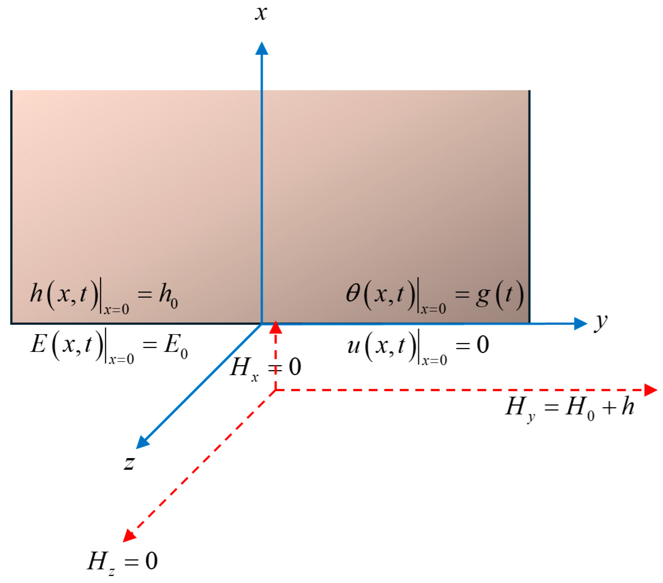
By assuming the space is occupied by an isotropic, generalized thermoelastic, electromagnetic, half-space, the magnetic vector field has been considered and acts tangent to the surface of the half-space when , and all the studied functions of the material are dependent only on one-dimension distance and the time variable .
gives the induced magnetic vector field due to the effect of the primary magnetic vector field
, then, an induced electric intensity vector field
will be generated as in
Figure 1 [
13,
28,
29,
30]:
We assume the vectors
and
have a small magnitude in the context of the linear generalized thermoelasticity theory of Green–Naghdi. Hence, the vector of displacement takes the following form:
The magnetic intensity vector takes the following components [
13,
28,
29,
30]:
Due to the role of the left-hand, the electric intensity vector field must be perpendicular to the displacement vectors and the magnetic intensity vector.
Hence, the electric field vector
has the following components:
Moreover, the current density vector
must be in the same direction as the electric intensity vector
. Thus, we have the following:
In general vector forms based on a fractional derivative definition, the time-fractional Maxwell’s equations can be written as follows [
23]:
and
The fractional-order time-derivative operator
will be applied in which the integer derivative
gives the free-space situation, and the Caputo fractional derivative when
, respectively, as in the following unified form [
14,
15,
16,
17,
18,
19,
20,
21,
22,
23,
24,
25,
26]:
where
and
give the magnetic and electric permeabilities, respectively [
2,
6,
13,
23,
31,
32].
Equations (5)–(9) are supported by Ohm’s law, namely [
2,
6,
13,
23,
31,
32] as follows:
Ohm’s law gives the following equation [
2,
6,
13,
23,
31,
32]:
where
gives the electric conductivity.
Lorentz’s force vector is given by the following law [
2,
6,
13,
23,
31,
32]:
Hence, from Equations (9), (12), and (13), we obtain the following:
After linearization, we obtain the following:
The strain components take the following forms [
13]:
and
The stress components are given by the following relation [
13]:
which has the following components [
13]:
and
where
defines the absolute temperature of the medium;
is a reference temperature assumed to be such that
;
and
are Lamé’s moduli;
; and
is the linear thermal expansion coefficient.
Equations of motion in general unified form are as follows [
1,
3,
4]:
where
gives the density of the material.
By inserting Equation (12) into Equation (9), we obtain the equation of motion in one-dimensional form as follows [
2,
6,
13,
29,
31,
32]:
By exciting the partial derivative concerning the variable
and using Equation (17), Equation (23) takes the following new form:
The one-dimensional heat conduction equation of Green–Naghdi of type-I and type-III takes the following unified form [
33,
34,
35]:
The unified form of Equation (25) can be applied to both type-I and type-III of the Green–Naghdi theorem as follows:
- (a)
provides Green–Naghdi type-I.
- (b)
provides Green–Naghdi type-III.
We may take as the main character of the Green–Naghdi theory, while gives the thermal conductivity, and denotes the specific heat at constant deformation.
Equation (5) for the current model takes the following form:
Substituting from Equation (12), we obtain [
23] the following:
Also, Equation (6) takes the following form [
23]:
By adding a one-order partial derivative with respect to the variable
for Equation (27) and using Equation (28), we obtain the following equation [
23]:
In addition, Equation (24) will take the following form [
23]:
The following dimensionless variables will be applied for simplifications as follows [
13,
28,
29,
36]:
After omitting the primes for ease, the preceding equations have been simplified to the following system of differential equations:
and
where
The constitutive relations will be reduced to the following forms:
and
where
.
The Laplace transform of Formula (10) and its derivatives are given by the following [
14,
15,
16,
17,
18,
19,
20,
21,
22,
23,
24,
25,
26]:
The initial conditions of the current model are given as follows:
After applying initial conditions, form (37) will be in the following simple form [
14,
15,
16,
17,
18,
19,
20,
21,
22,
23,
24,
25,
26]:
Then, we have the following:
and
where
The constitutive equations are given by the following:
and
By eliminating the three functions
from Equations (40)–(42), we have the following characteristic equations:
where
, and
.
The solutions of Equation (46) bounded for
have the following forms:
and
where
are the roots of the characteristic equation:
By inserting Equations (47)–(49) into Equations (40)–(42), we obtain the following relations:
and
Then, we have the following:
and
Then, from the Equations (16) and (53), we have the following:
From Equations (43) and (54), we obtain the following:
To obtain the parameters , the following boundary conditions at the bounding surface of the half-space will be applied as follows:
- 1.
The half-space connected to a rigid foundation enough to prevent the displacement of the material is the mechanical boundary condition, i.e.,
- 2.
The surface of the half-space
loaded thermally by ramp-type heat gives the thermal boundary condition, which is defined as follows:
where
is called the ramp-time heat parameter and
is constant.
Applying the Laplace transform, the above condition takes the following form:
- 3.
The magnetic and electric functions
and
must satisfy the continuity conditions around the surface
and give the magnetic and electrical boundary conditions as follows [
13]:
and
where
give the magnetic and electric intensities in the free space, respectively.
In the free space, in the non-dimensional Maxwell’s equations in the Laplace transform domain, we can put
, which give the following equations:
and
Eliminating
between the above two equations, we obtain the following:
where
.
The bounded solution of Equation (64) in a general form is given by the following:
From Equations (63) and (65), we obtain the following:
From Equations (62) and (66), we obtain the condition when
as [
13] follows:
Applying the boundary conditions (57), (59), and (67), we obtain the following system of linear equations in the unknown parameters
:
and
Solving the system of linear Equations (68)–(70) gives complete solutions in the domain of the Laplace transform.
3. The Numerical Results and Discussion
The Laplace transform inversions may be determined using the iteration form indicated in the following equation [
37]:
gives the unit of an imaginary number, while “
” provides the real part of any complex function, and
is an integer parameter that could be chosen such that the following applies:
To get a faster convergence for the above iteration, the parameter “
“ may satisfy the following condition:
[
37,
38].
Copper material has been used for the numerical calculations. The properties of the material and the parameters have been taken as follows [
2,
6,
13,
29,
30,
32]:
The dimensionless dimension variable has been taken as follows: .
Figure 2,
Figure 3,
Figure 4,
Figure 5,
Figure 6 and
Figure 7 show the distributions of the temperature increment, the volumetric dilatation, displacement, stress, induced magnetic field, and induced electric field based on Green–Naghdi type-I and type-III, respectively, under the definition of the fractional-order derivative of Caputo for three different values of the fractional-order parameter where
gives the traditional material of normal derivative, while
gives the time-fractional Maxwell’s equations cases. The results have been obtained based on two different cases of the ramp-time heat parameter
to stand on this parameter’s effects on all the studied functions.
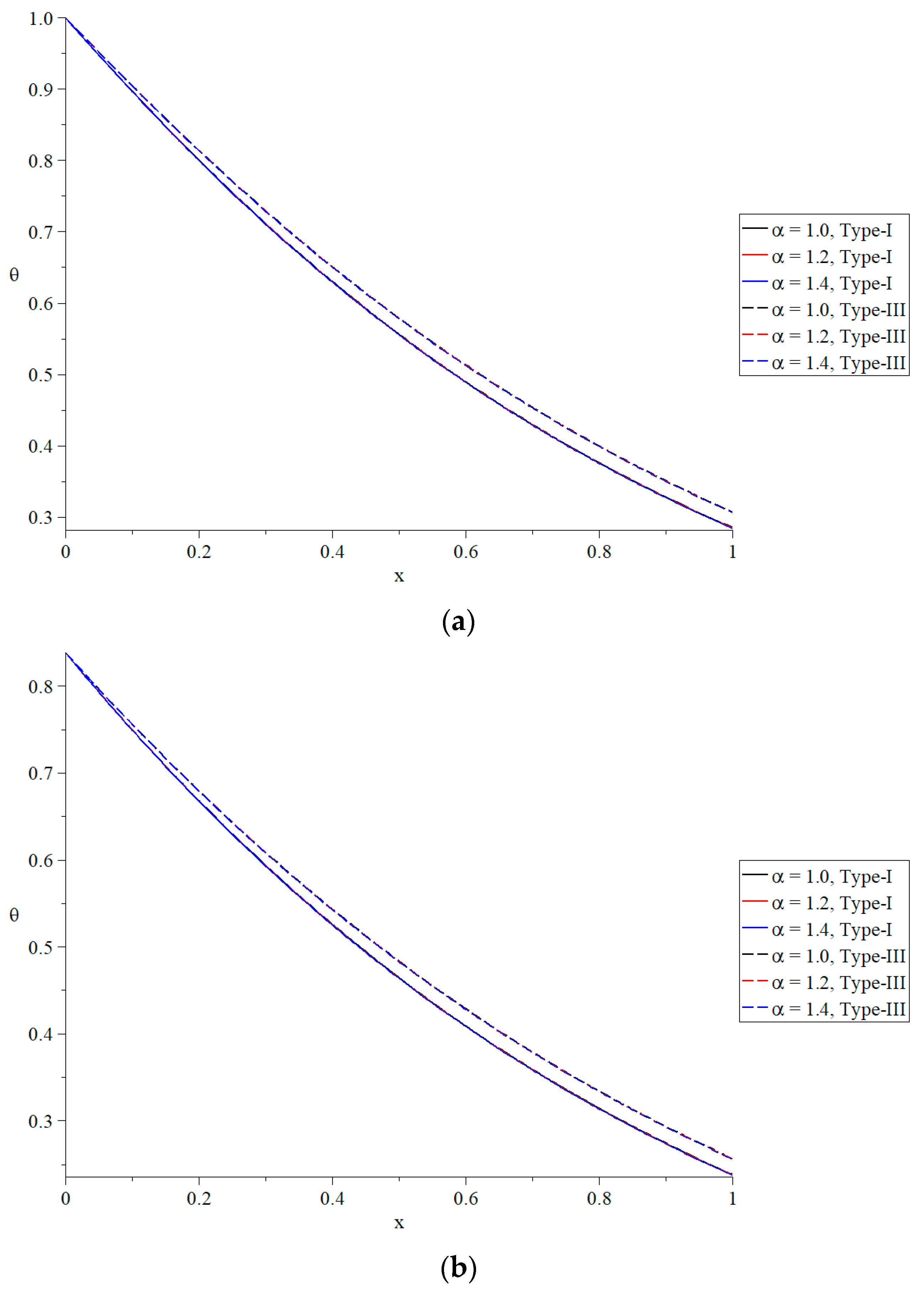
Figure 2 depicts the impact of the time-fractional parameter in Maxwell’s equations on the temperature increment distribution, revealing a minimal effect.
Figure 2a,b illustrate that the ramp-time heat parameter significantly influences the temperature increment, whereas an increase in the ramp-time heat parameter correlates with a reduction in the temperature increment. Moreover, the values of the temperature increment under Green–Naghdi type-I and type-III take the following order:
which means that the thermal wave based on Green–Naghdi type-I propagates with a more limited speed than type-III.
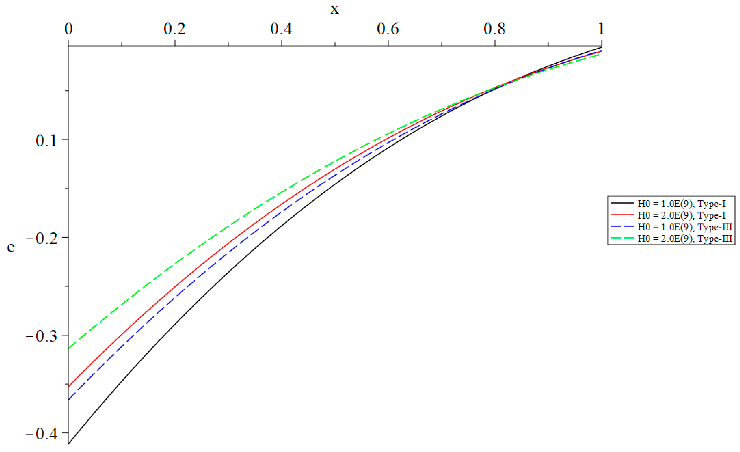
The effects of the time-fractional parameter on the volumetric dilatation distribution are shown in
Figure 3, which indicates that the volumetric dilatation distribution is significantly affected. Within both categories shown in
Figure 3a,b, it can be seen that an increase in the time-fractional parameter of Maxwell’s equations results in a reduction in the absolute value of volumetric dilatation. When compared to the results obtained from Green–Naghdi type-III, the volumetric dilatation values obtained from Green–Naghdi type-I are superior. Within the framework of Maxwell’s equations, the time-fractional parameter functions as a resistor to the deformation of the material. There is a considerable relationship between the ramp-time heat parameter and the distribution of volumetric dilatation; an increase in this parameter leads to a decrease in the absolute value of volumetric dilatation.
The absolute values of the volumetric dilatation take the following order:
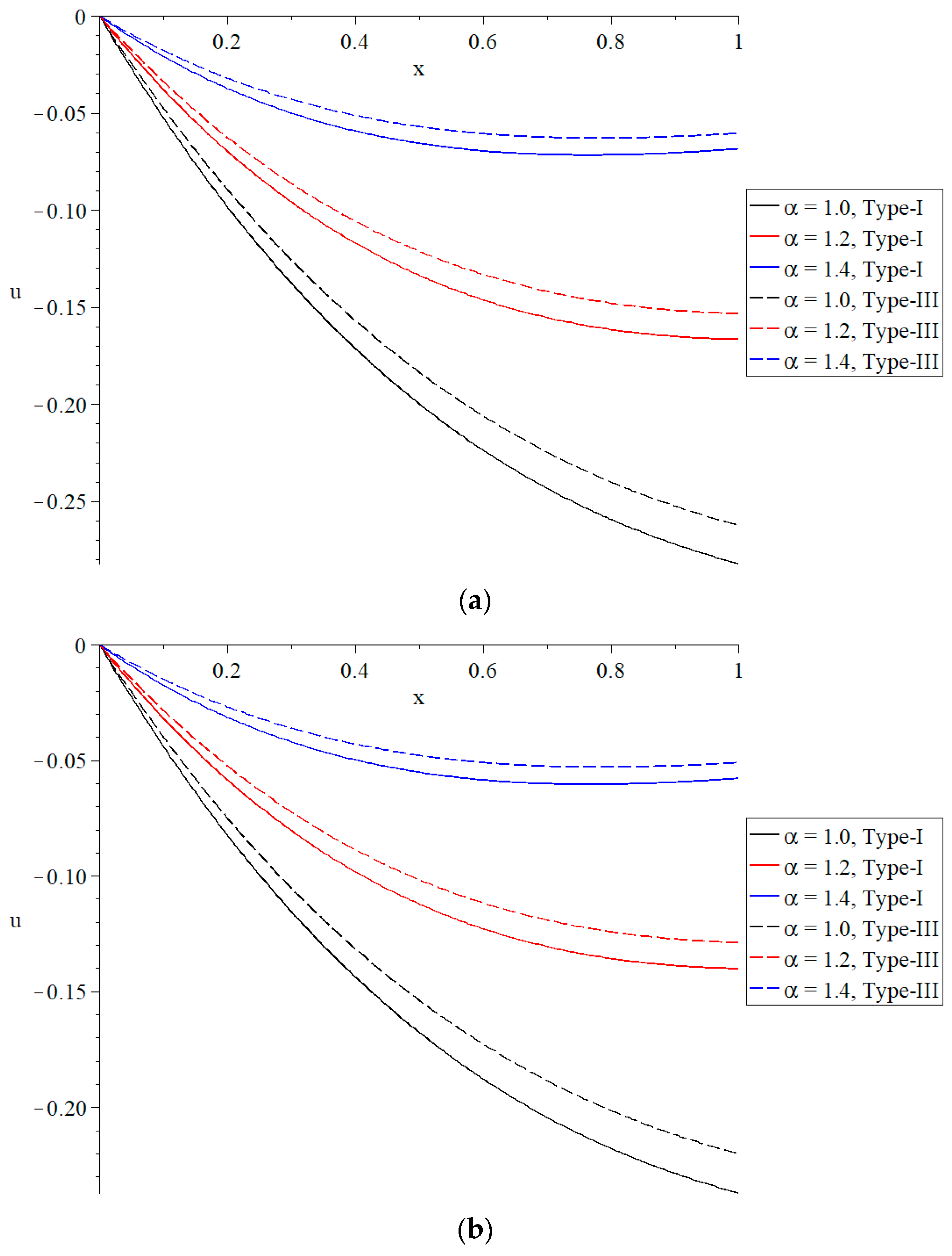
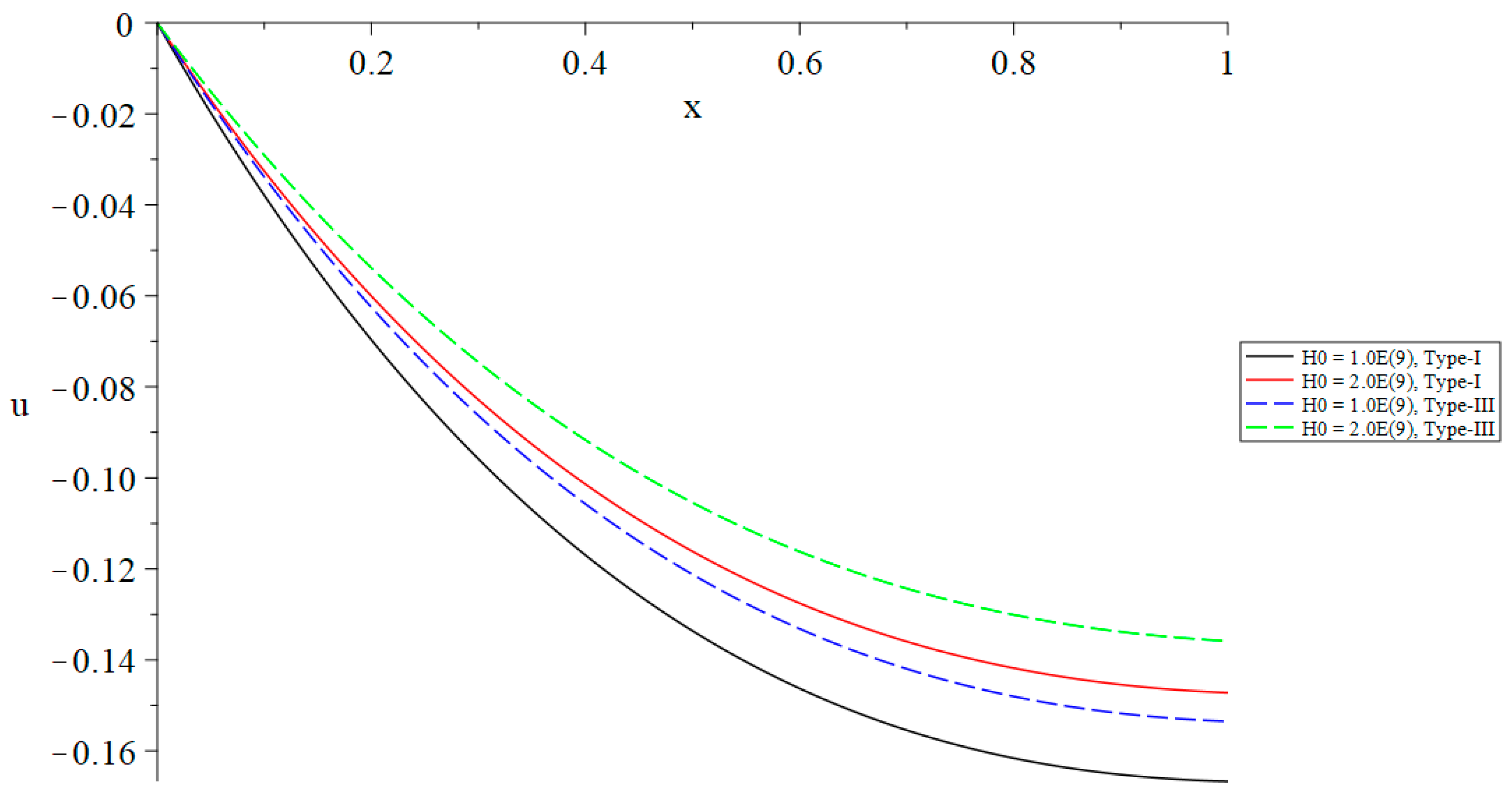
The influence that the time-fractional parameter has on the distribution of displacement is seen in
Figure 4, which may be found here. The magnitude of this influence is significant; as can be seen in
Figure 4a,b, an increase in the time-fractional parameter results in a reduction in displacement for both species that were investigated. There is a significant improvement in the displacement values obtained from Green–Naghdi type-I in comparison to those obtained from Green–Naghdi type-III. A further purpose of the time-fractional parameter in Maxwell’s equations is to serve as a resistor to the movement of particles inside the medium. A decrease in the absolute displacement value is the consequence of an increase in the value of the ramp-time heat parameter, which has a substantial impact on the distribution of displacement. The absolute values of the displacement take the following order:
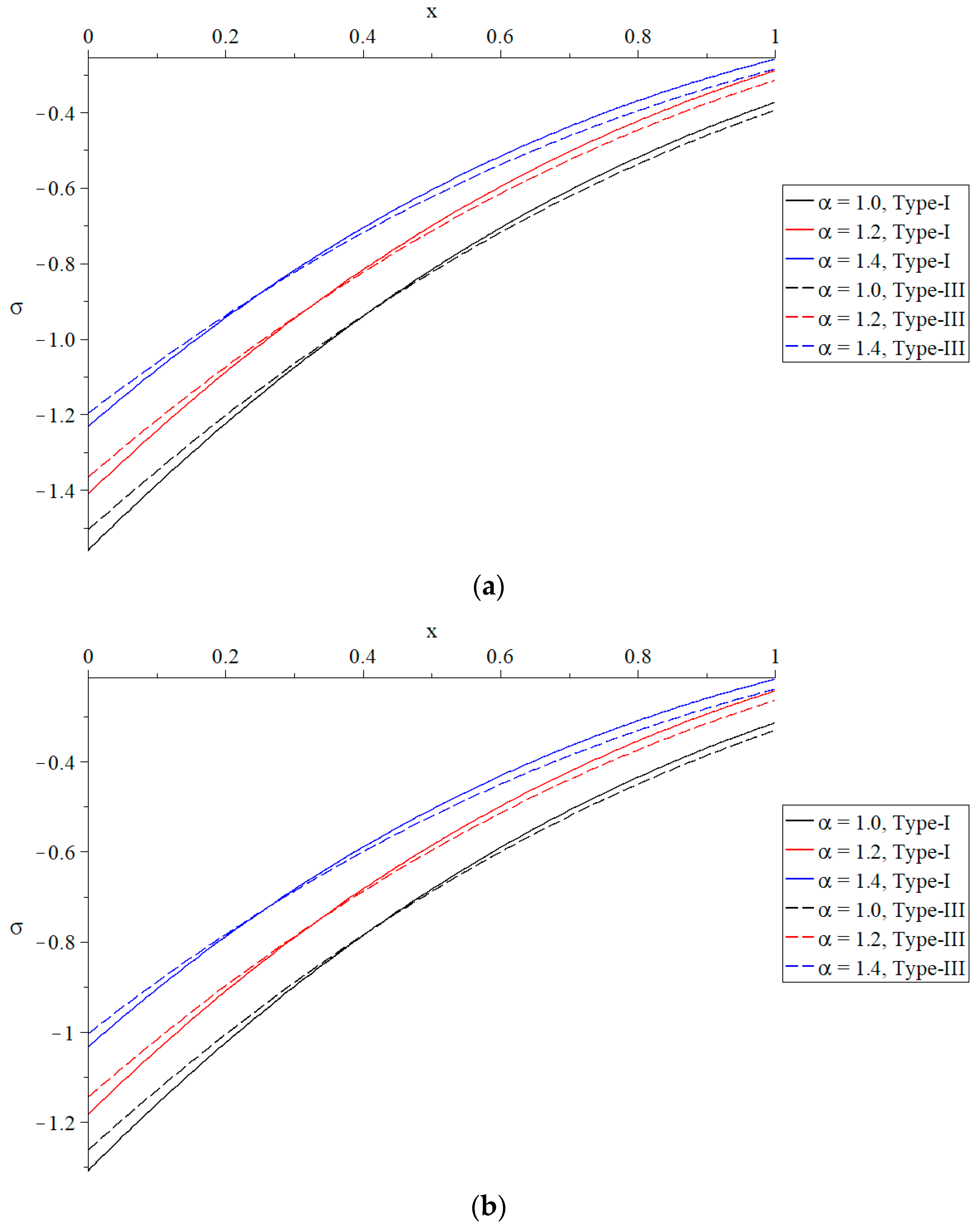
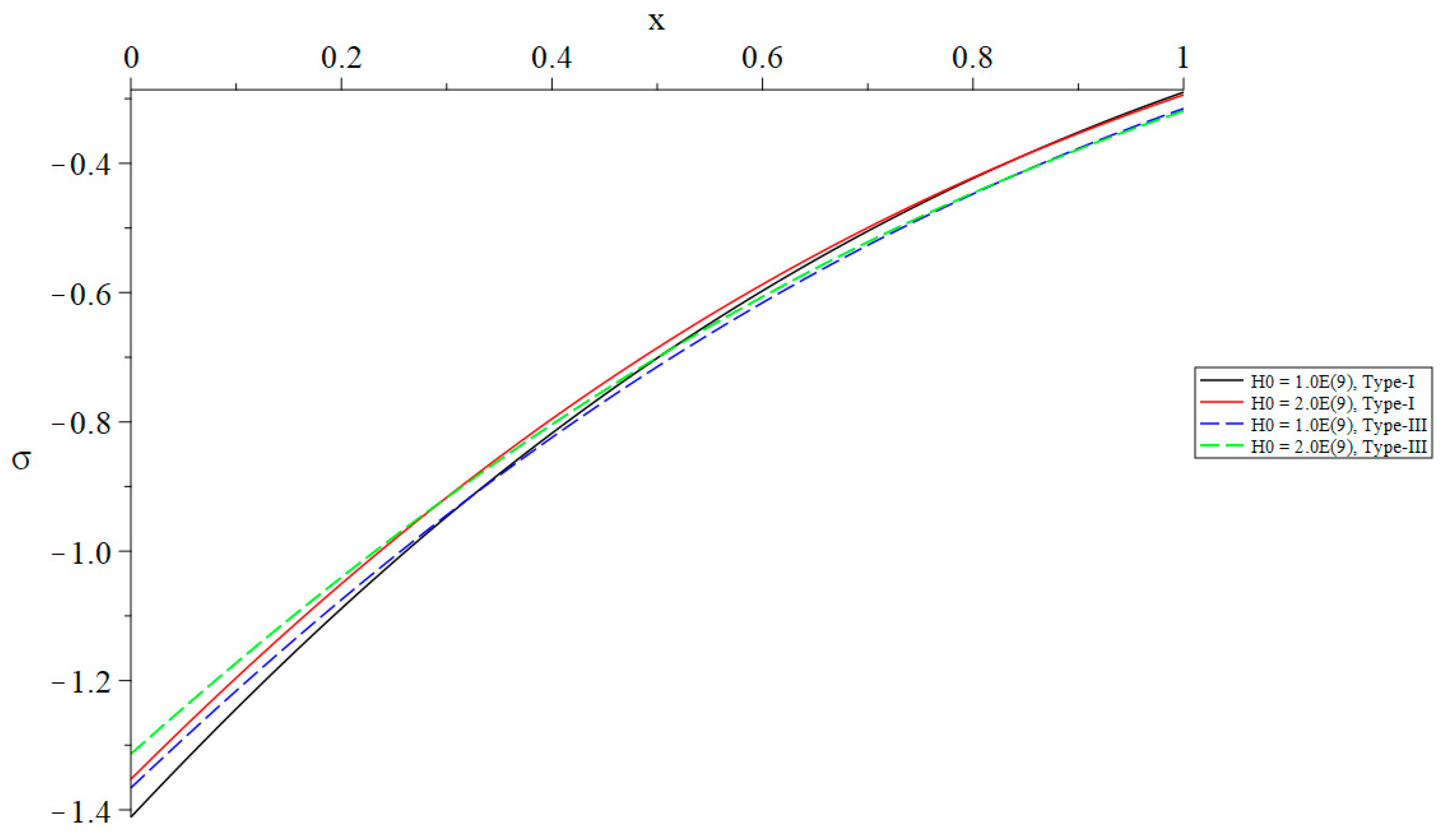
The influence of the time-fractional parameter in Maxwell’s equations on the distribution of stress is seen in
Figure 5, which reveals that the effect is both significant and continuously growing. There is a correlation between a rise in the time-fractional parameter and an increase in the absolute stress value at the boundary surface as can be observed in both types of stress that are shown in
Figure 5a,b. In comparison to Green–Naghdi type-III, the absolute levels of stress that were acquired from Green–Naghdi type-I were determined to be higher. In addition, the ramp-time heat parameter has a significant impact on the distribution of stress, and an increase in its value leads to a decrease in the relative magnitude of the absolute stress. The absolute values of the stress on the bounding plane of the half-space
take the following order:
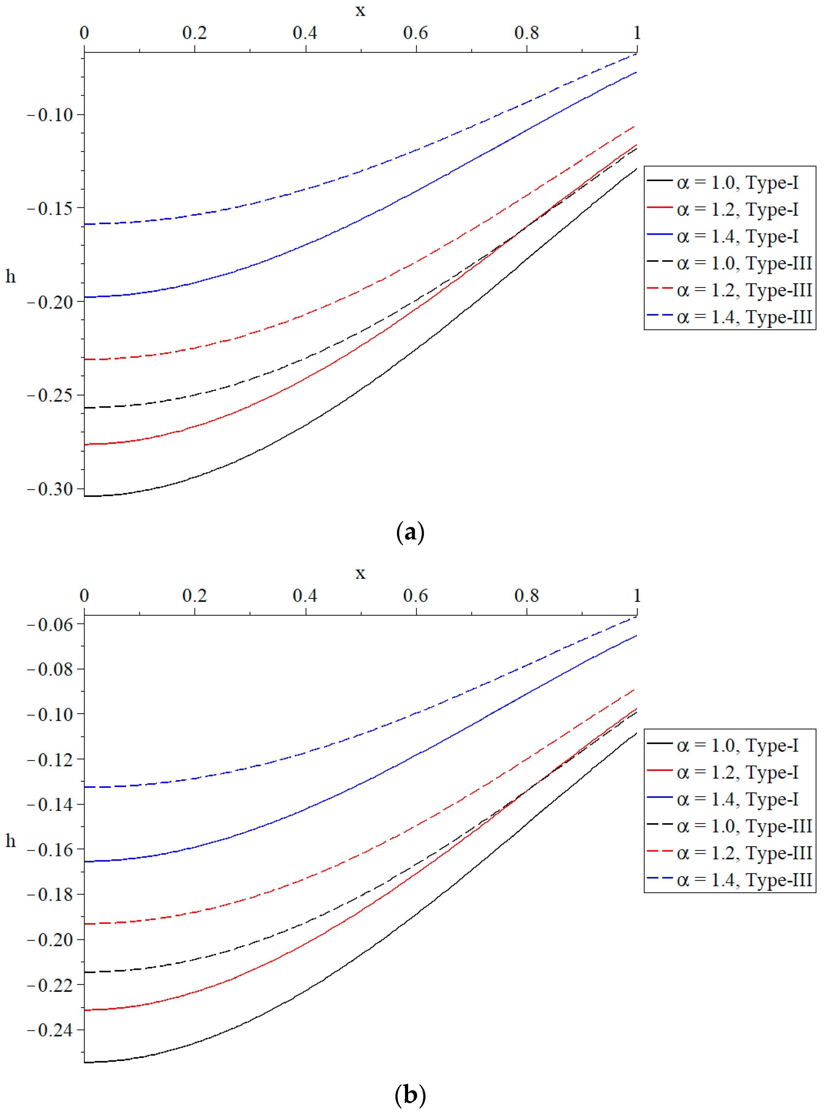
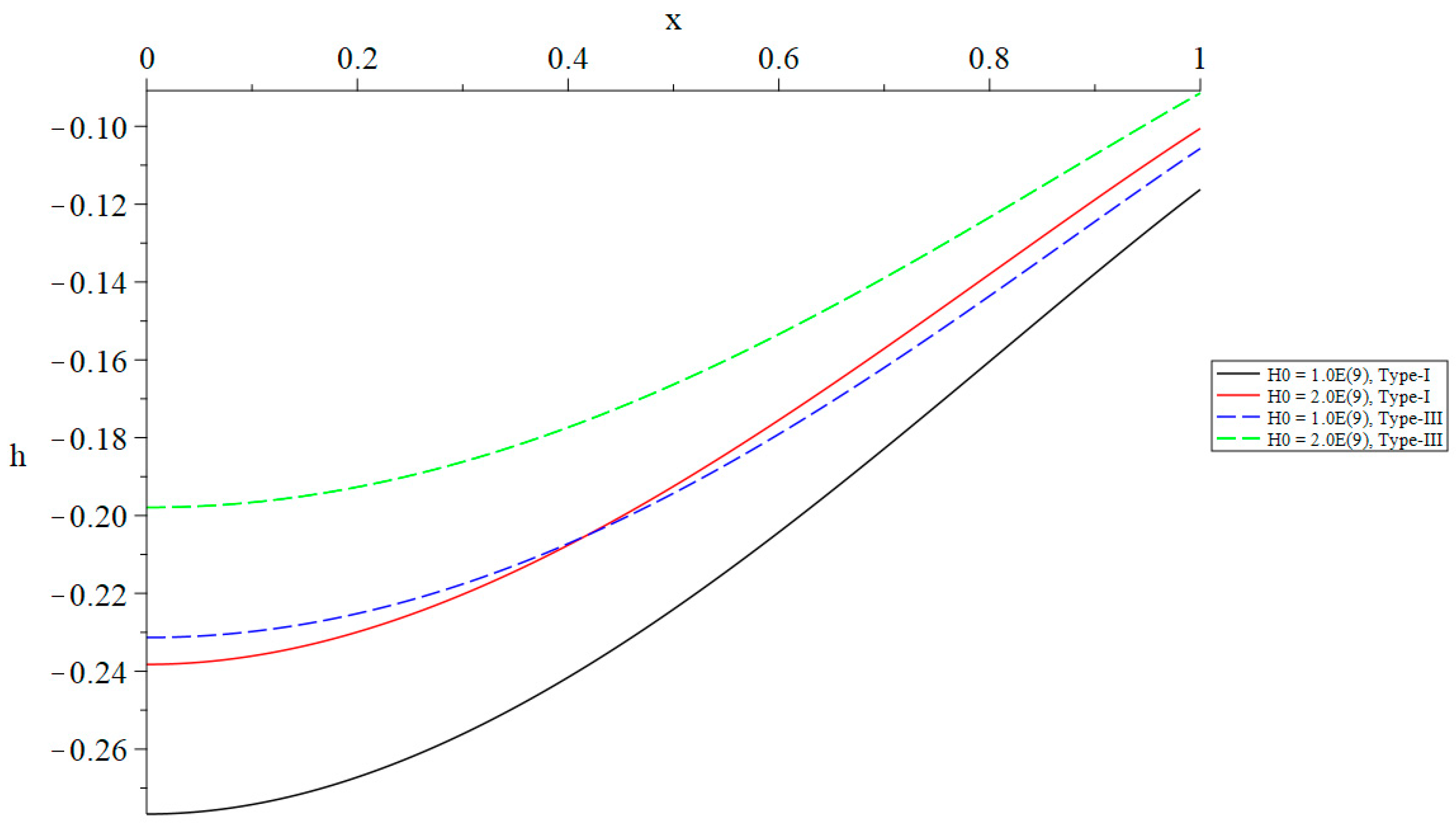
The influence that the time-fractional parameter in Maxwell’s equations has on the distribution of the magnetic field that is created is seen in
Figure 6. An increase in the time-fractional parameter results in a reduction in the induced magnetic field as can be seen in
Figure 6a,b for both kinds that were investigated. This is a considerable influence. When compared to the values generated by Green–Naghdi type-III, the induced magnetic field values that are acquired from Green–Naghdi type-I may be considered better. Maxwell’s equations include a time-fractional parameter that functions as a barrier to the magnetic field that is created inside the material under consideration. In addition, the ramp-time heat parameter has a major impact on the distribution of the magnetic field that is created. Furthermore, an increase in the value of this parameter leads to a decrease in the absolute magnitude of the magnetic field that is induced. The absolute values of the induced magnetic field take the following order:
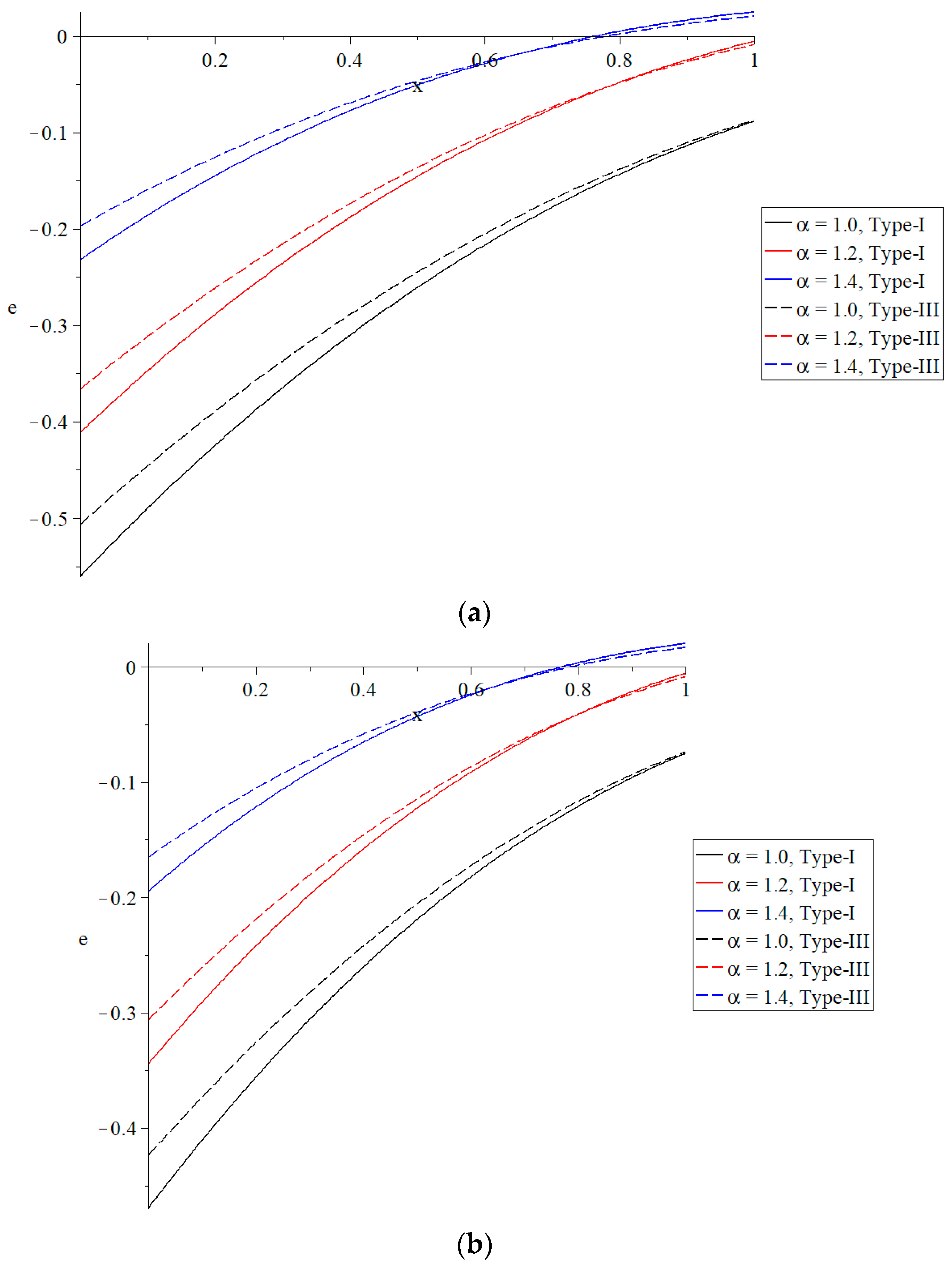
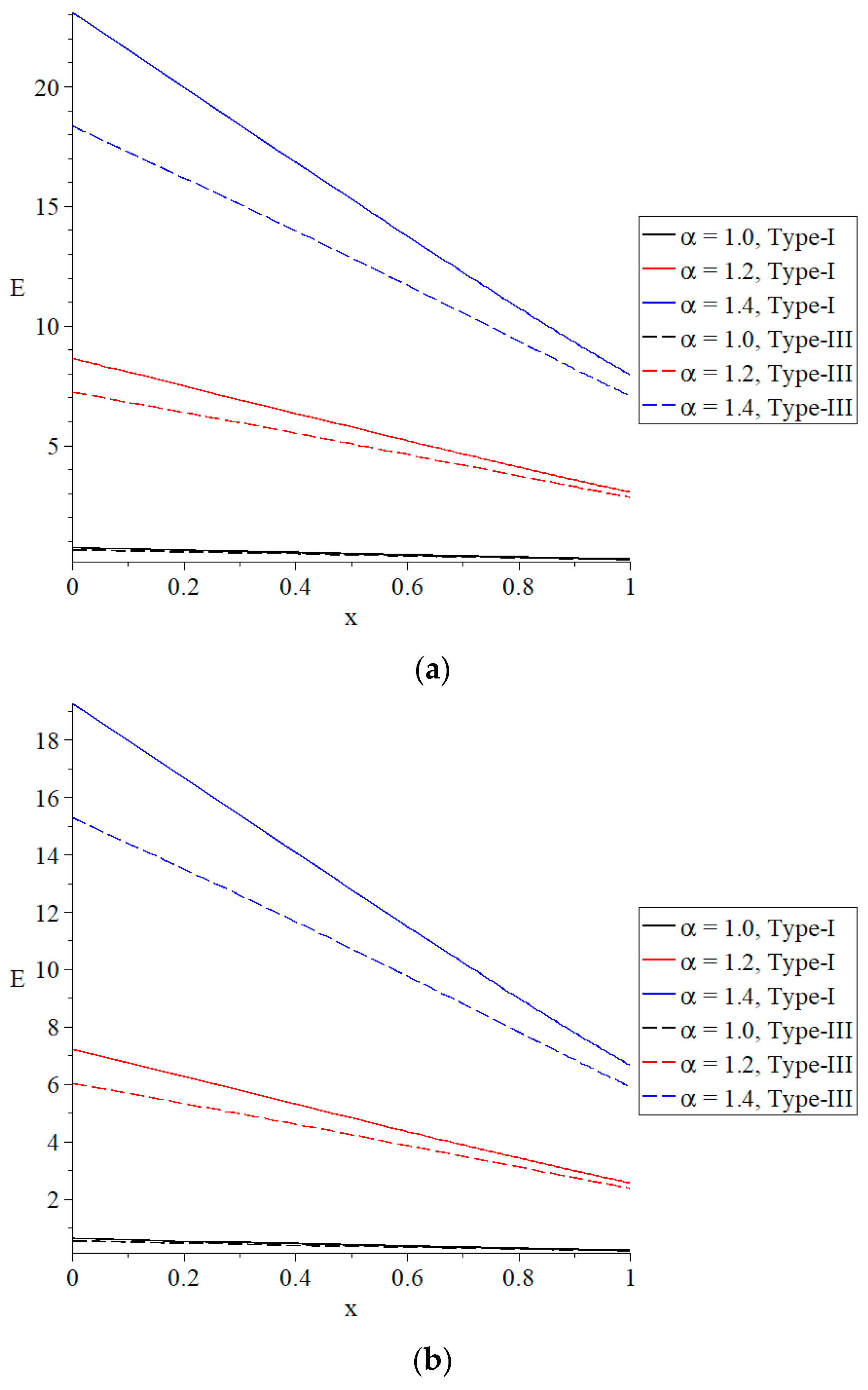
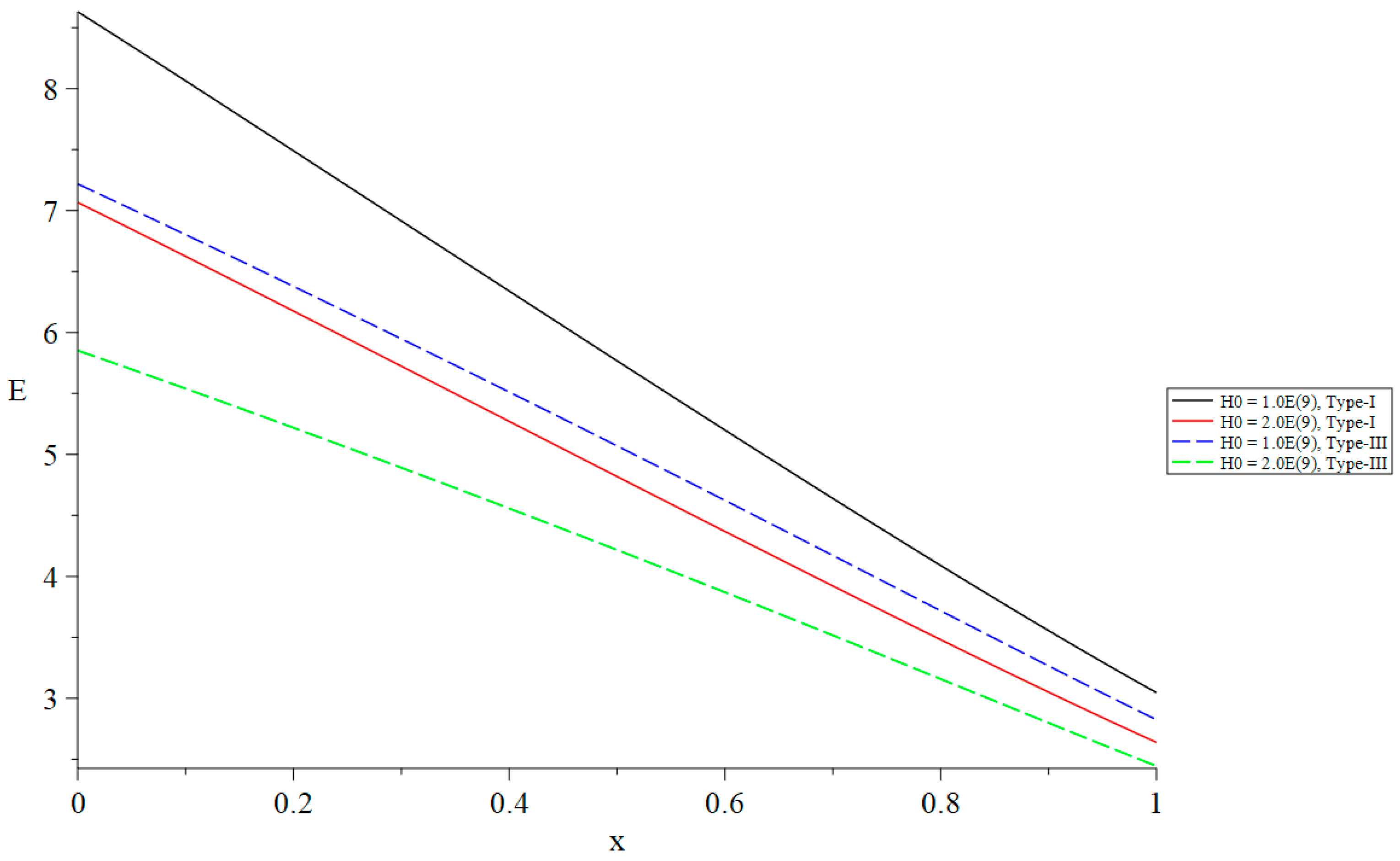
The influence that the time-fractional parameter in Maxwell’s equations has on the distribution of the electric field that is created is seen in
Figure 7. As can be observed in
Figure 7a,b, the influence is significant; an increase in the time-fractional parameter coincides with an elevation in the generated electric field. This is the case for both kinds that were investigated. When compared to the values obtained from Green–Naghdi type-III, the induced electric field values obtained from Green–Naghdi type-I are exceptional. The creation of the induced electric field inside the material is made easier by the time-fractional parameter that is included in Maxwell’s equations. To add insult to injury, the ramp-time heat parameter has a substantial impact on the distribution of the produced electric field. As a consequence, a rise in its value leads to a decrease in the intensity of the induced electric field. The values of the induced electric field take the following order:
Figure 8,
Figure 9,
Figure 10,
Figure 11,
Figure 12 and
Figure 13 show the distributions of the temperature increment, the volumetric dilatation, displacement, stress, induced magnetic field, and induced electric field based on Green–Naghdi type-I and type-III, respectively, under the definition of the fractional-order derivative of Caputo when
with different values of the primary magnetic field
.
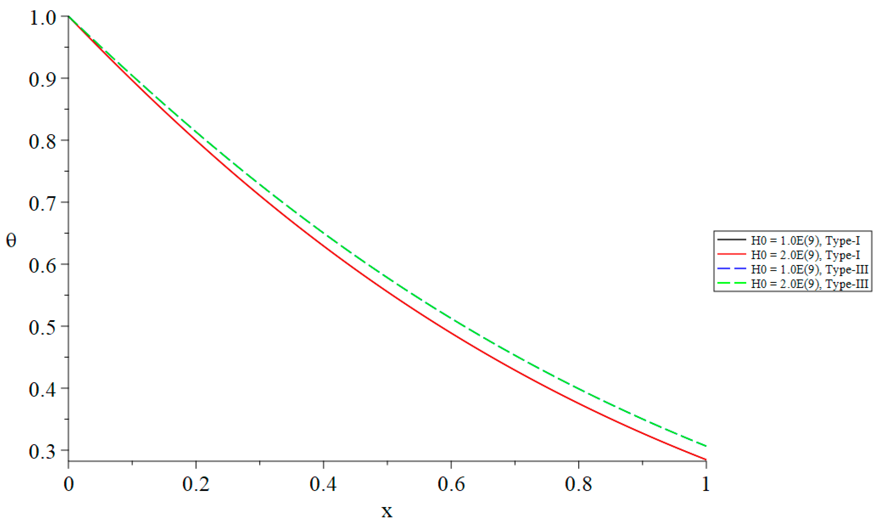
In
Figure 8, it is shown that the primary magnetic field has a negligible impact on the temperature rise.
Figure 9 demonstrates that the primary magnetic field has a significant impact on volumetric dilatation. Specifically, an increase in the primary magnetic field is correlated with a decrease in the absolute value of volumetric dilatation. An increase in the primary magnetic field is correlated with a decrease in the absolute value of the displacement as shown in
Figure 10. This indicates that the primary magnetic field has a significant impact on displacement. An increase in the primary magnetic field is correlated with a decrease in the absolute magnitude of stress as shown in
Figure 11. This demonstrates that the primary magnetic field has a significant impact on stress.
Figure 12 demonstrates that the primary magnetic field has a significant impact on the induced magnetic field. This influence is such that an increase in the magnitude of the primary magnetic field leads to a decrease in the absolute value of the induced magnetic field. It is shown in
Figure 13 that the primary magnetic field has a significant impact on the electromagnetic field. Specifically, a rise in the primary magnetic field is correlated with a decrease in the induced electric field.
5. Conclusions
Within the scope of this study, a novel and distinct mathematical model of a generalized magnetothermoelastic half-space with a single thermal relaxation period was presented. Taking into consideration time-fractional Maxwell’s equations, the model was constructed using Green–Naghdi theory type-I and type-III as its theoretical foundation. This model makes use of the definition of the Caputo fractional derivative, which is the fractional derivative that has been applied. It was determined that direct use of Laplace transform methods was the most effective method for this. For calculating the inverse Laplace transform, the iteration method that Tzou had created was used. It has been determined and described how the distributions of temperature increment, strain, displacement, stress, induced magnetic field, and induced electric field are distributed. These distributions have been determined and explained.
The distributions of temperature increment, strain, displacement, stress, induced magnetic field, and induced electric field based on Green–Naghdi type-I and type-III are significantly influenced by the time-fraction parameter in Maxwell’s equations. This is the case because the time-fraction parameter has a significant effect.
More than any other parameter, the time-fraction parameter has the greatest impact on these distributions.
The time-fractional parameter of Maxwell’s equations functions as a resistor to the movement of the particle, volumetric dilatation, and the induced magnetic field. On the other hand, it functions as a catalyst for the induced electric field that is present inside the material.
Thermal, mechanical, and magnetoelectric waves are all significantly impacted by the ramp-time heat parameter due to their considerable implications.
When it comes to mechanical and magnetoelectric waves, the ramp-time heat parameter has a substantial impact, although it has no impact whatsoever on the thermal temperature wave.
The pace at which thermal, mechanical, and magnetoelectric waves propagate under Green–Naghdi type-III is slower than the speed at which type-I waves propagate.
There are considerable effects that the main magnetic field has on all of the functions that were investigated.


