Abstract
Emotion recognition based on Electroencephalogram (EEG) signals plays a vital role in affective computing and human–computer interaction (HCI). However, noise, artifacts, and signal distortions present challenges that limit classification accuracy and robustness. To address these issues, we propose ECA-ResDNN, a novel hybrid model designed to leverage the frequency, spatial, and temporal characteristics of EEG signals for improved emotion recognition. Unlike conventional models, ECA-ResDNN integrates an Efficient Channel Attention (ECA) mechanism within a residual neural network to enhance feature selection in the frequency domain while preserving essential spatial information. A Deep Neural Network further extracts temporal dependencies, improving classification precision. Additionally, a hybrid loss function that combines cross-entropy loss and fuzzy set loss enhances the model’s robustness to noise and uncertainty. Experimental results demonstrate that ECA-ResDNN significantly outperforms existing approaches in both accuracy and robustness, underscoring its potential for applications in affective computing, mental health monitoring, and intelligent human–computer interaction.
MSC:
68T07
1. Introduction
Emotion is a psycho-physiological process triggered by conscious or unconscious perceptions of objects or situations and is often linked with feelings, temperament, personality, and motivation [1]. Emotion recognition has emerged as a critical research area in human–computer interaction and affective computing, with vast application prospects in fields such as human–computer interaction, psychotherapy, and education [2,3,4,5,6,7,8,9]. In recent years, emotion recognition based on electroencephalogram (EEG) signals has gained significant attention as EEG provides physiological data that directly reflects human emotional states. It offers advantages such as resistance to external interference and high spatiotemporal resolution [10,11].
Prior to the widespread adoption of deep learning in EEG research, several automatic or semi-automatic EEG recognition methods had been proposed [12,13,14,15,16]. With the rise of deep learning techniques, a growing number of scholars have applied these methods to emotion recognition, which surpass the performance of traditional approaches and achieve results previously unattainable. For example, Tripathi et al. [17] proposed using Convolutional Neural Networks (CNNs) to estimate functions that are dependent on a large number of typically unknown inputs, which classify users’ emotions using EEG data from the DEAP dataset. This approach outperformed the Support Vector Machine (SVM) binary classification model [3] by 4.51% and 4.96% on the valence and arousal dimensions, respectively, and surpassed emotion classification methods based on Bayesian classifiers and supervised learning [18] by 13.39% and 6.58%. These findings demonstrate that neural networks can serve as powerful classifiers for brain signals, surpassing traditional learning techniques. In the same year, Al-Nafjan et al. [19] proposed the use of Deep Neural Networks (DNNs) for recognizing user emotions from power spectral density (PSD) and frontal asymmetry features in EEG signals, which achieved an average identification accuracy of 82.0% for binary classification on the DEAP dataset. This highlights the significant performance improvement of emotion recognition using DNNs, especially when large training datasets are available.
Attention mechanisms play an indispensable role in human perception, particularly in filtering, integrating, and interpreting information [20]. In traditional deep learning models, feature fusion is often achieved through simple operations like weighted averaging or concatenation, which may not fully capture the differences in importance among various features. The integration of attention mechanisms allows models to learn the relevance of features automatically and adjust their weights based on their importance, resulting in more effective feature fusion. Liu et al. [21] introduced the 3DCANN model, which incorporated an EEG channel attention learning module to extract discriminative features from continuous multi-channel EEG signals, highlighting the variability of EEG signals across different emotional states. Tao et al. [22] proposed the ACRNN model, which integrated self-attention mechanisms into Recurrent Neural Networks (RNNs) to focus on the temporal information in EEG signals, adaptively assigning weights to different channels via a channel-wise attention mechanism. Zhang et al. [23] proposed a novel two-step spatial-temporal emotion recognition framework, combined local and global temporal self-attention networks to improve recognition performance, and introduced a new emotion localization task to identify segments with stronger emotional signals. Building on the development of attention mechanisms, Liu et al. [24] explored the use of Transformer-based multi-head attention mechanisms, proposing four variant transformer frameworks to investigate the relationship between emotions and EEG spatial-temporal features, thus demonstrating the importance of modeling spatial-temporal feature correlations for emotion recognition. These studies clearly indicate that incorporating attention mechanisms can substantially enhance recognition performance.
In this paper, we propose a novel hybrid model for EEG-based emotion recognition, named ECA-ResDNN. The main contributions of this work are as follows:
- To address challenges such as noise, artifacts, discontinuities, drift, and distortion in EEG signal data, we introduce a novel preprocessing method that integrates Generative Adversarial Networks (GANs) and fuzzy set theory. This approach enhances the clarity and stability of EEG signals, improving the accuracy and robustness of the algorithm.
- A novel Deep Neural Network is employed for EEG-based emotion recognition, leveraging its ability to capture intricate features within EEG signals. Additionally, an attention mechanism is incorporated to enhance the model’s sensitivity and ability to differentiate emotional information. This combination enables the model to better interpret and represent the emotional content of EEG signals, leading to more accurate and reliable emotion recognition.
- To further enhance the robustness and accuracy of the classification model in handling uncertainty and noisy data, we propose a hybrid loss function that integrates cross-entropy loss with fuzzy set loss. This approach aims to combine the efficiency of cross-entropy loss in classification tasks with the advantages of fuzzy set loss in dealing with noise and uncertainty.
Comparative experiments were conducted against classical models, including CNNs, CNN-GRU, CNN-LSTM, and DNNs, as well as state-of-the-art methods such as SPD + SVM [25] and GLFANet [26]. The results demonstrate that ECA-ResDNN achieves superior accuracy and robustness compared to existing emotion recognition models. These findings validate the effectiveness of the proposed hybrid model in enhancing classification performance.
2. Materials and Methods
2.1. DEAP Dataset
The DEAP dataset was created by Koelstra et al. [1] from Queen Mary University of London in collaboration with other institutions. EEG signals were recorded using the ActiveTwo system, manufactured by Biosemi B.V., located in Amsterdam, The Netherlands, with 32 active AgCl electrodes placed according to the international 10–20 system and a sampling rate of 512 Hz [27]. In addition to EEG, peripheral physiological signals were also recorded, including EOG (electrooculography, with four facial electrodes capturing eye movement signals) and EMG (electromyography, with four electrodes placed on the zygomaticus major and trapezius muscles to capture muscle activity signals). Furthermore, physiological sensors were placed on the left hand, measuring pulse oximetry, temperature, and galvanic skin response (GSR).
A total of 32 participants (16 males and 16 females, aged between 19 and 37 years, with a mean age of 26.9 years) were recruited. All participants were in good physical and mental health, had no history of neurological or psychiatric disorders, and were all right-handed. Prior to the experiment, participants were required to read and acknowledge the experimental instructions and procedures. The instructions included guidelines on minimizing movement artifacts and emotional tension, which could introduce noise into EEG recordings. During the experiment, each participant watched 40 one-minute video clips sequentially while their EEG data were recorded in real-time. The data collection process for the DEAP dataset is illustrated in Figure 1.
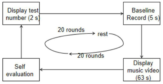
Figure 1.
DEAP data collection process flowchart.
In each experimental session, the current experiment number was displayed to inform participants of their progress. This was followed by a five-second baseline recording to capture initial brain activity. Subsequently, a one-minute music video was presented, forming the core of the experimental procedure. After the video, participants were asked to self-assess their arousal, valence, and other emotional states, with their responses reflecting various affective conditions. To minimize fatigue and ensure data accuracy, participants took short breaks every 20 trials, during which experimental equipment and electrode placements were checked and adjusted if necessary.
2.2. Data Augmentation
The Wasserstein Generative Adversarial Network (WGAN) [28] is an advanced architecture within the framework of Generative Adversarial Networks (GANs) that introduces the Wasserstein distance as a new metric to measure the discrepancy between generated and real samples. Unlike the commonly used Jensen–Shannon (JS) divergence [29] in traditional GANs, the Wasserstein distance has been shown to perform more effectively, particularly in the field of emotion recognition [30]. As illustrated in Figure 2, Q and P represent the probability distributions of the generated and real samples, respectively. The arrow represents the transformation of the probability distribution of generated samples (Q) towards the real samples (P) in the Wasserstein distance framework. To transform Q into P, one can imagine using a bulldozer to move the “dirt” (i.e., probability mass) within Q, gradually reshaping it to match P. The average shortest distance the bulldozer must travel during this process is defined as the Wasserstein distance, mathematically expressed as follows:
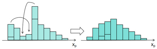
Figure 2.
Wasserstein Distance.
In Equation (1), π() represents the set of all possible joint distributions γ between the real distribution and the generated distribution . denotes the distance between a real sample x and a generated sample y, and E(x,y) is the expected value of this distance for the pair of samples.
During the training process, two distinct loss functions are utilized—one for the discriminator and one for the generator—as follows:
2.3. Data Preprocessing
In this study, EEG signals from 32 channels of the DEAP dataset are initially selected. After configuring the electrode layout and reference signal, a 50 Hz notch filter and a 4–45 Hz band-pass filter are applied to remove noise and highlight the frequency components of interest, thereby enhancing the signal quality. To further improve signal purity, Independent Component Analysis (ICA) and wavelet transform are applied to remove ocular and muscle artifacts. Following this, based on event information extracted from the stimulus channel and a specified time window, the raw EEG data are segmented into a series of epochs with a window size of 2 s and a step size of 0.125 s.
Next, the Fuzzy C-Means (FCM) [31] algorithm is employed to cluster the epoch data, remove noise components, and downsample the signals to a target sampling frequency of 128 Hz. Unlike traditional filtering methods that rely on predefined basis functions, FCM utilizes soft clustering to assign membership probabilities to each data point, enabling a more flexible and adaptive noise removal process. This characteristic is particularly advantageous for EEG signals, which exhibit high variability and overlapping frequency components. The processed EEG signal spans 63 s and consists of 3 s of transition time between video segments and 60 s of actual video stimulus presentation. The objective function of FCM is defined as follows:
In Equation (4), n represents the number of data points, c is the number of clusters, is the degree of membership of the i-th data point in the j-th cluster, m is the fuzziness parameter, is the i-th data point, and is the center of the j-th cluster.
The power spectral density (PSD) plots of the epoch data after noise removal and downsampling are shown in Figure 3. The colors of the dots represent different EEG channels, while the lines corresponding to each color indicate the variation in power spectral density (PSD) for the respective channels. For each epoch, the EEG signal from the 3 s video transition period is used as a baseline to eliminate any EEG activity unrelated to the video stimulus. This results in a 60 s EEG signal sequence. Subsequently, feature extraction is performed on the processed data.
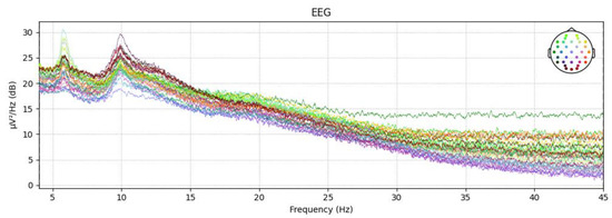
Figure 3.
PSD plot of the epochs data after noise removal and downsampling.
2.4. Feature Extraction
The Fast Fourier Transform (FFT) is an efficient algorithm for the Discrete Fourier Transform (DFT) [32], enabling the rapid conversion of time domain signals into frequency-domain signals. If the input time domain signal satisfies the following condition
then can undergo a continuous Fourier transform with the following formula:
In Equation (6), represents the output frequency signal, is the frequency, and i is the imaginary unit. However, since both the time domain and frequency domain signals are discrete in digital signal processing, the continuous Fourier transform is not directly computable on a computer. Therefore, the Discrete Fourier Transform (DFT) is commonly used. For a discrete signal sample , the DFT result is given by the following:
In Equation (7), N is the length of the signal, and is the frequency index, ranging from 0 to .
The Fast Fourier Transform (FFT) takes advantage of the symmetry, periodicity, and reducibility of Fourier coefficients to optimize the calculation of the DFT, significantly improving computational efficiency. The basic FFT algorithms are divided into two main types: the time-decimation method and the frequency-decimation method. This design employs a time-window-based approach. Assuming that the data within the k-th time window are represented as , the spectrum is computed as follows:
In Equation (8), is the number of sampling points within each time window.
To mitigate noise, spikes, and interference while preserving the relevant signal information, a Least Mean Square (LMS) filter is applied in this design. The filter updates its coefficients based on the error between the input signal and the desired output, minimizing the mean square error. The weight update rule is the following:
In Equation (9), is the learning rate, is the prediction error, and is the input signal vector.
Additionally, window functions are widely used in spectral analysis to effectively suppress the effects of signal truncation and improve processing accuracy. In this design, the Hanning window is selected due to its ability to balance spectral resolution and leakage suppression, making it particularly suitable for EEG signals with overlapping frequency components. The formula for the Hanning window is the following:
In Equation (10), represents the window length, and denotes the index of the sample point within the window. A longer window provides higher frequency resolution but may blur temporal details, while a shorter window improves temporal resolution but increases spectral leakage. is carefully selected based on the EEG sampling rate and epoch segmentation to ensure an optimal trade-off between frequency resolution, temporal precision, and noise suppression.
Finally, all feature vectors and labels are saved as .npy files. The results of feature extraction for the EEG signal data from the first participant are shown in Figure 4.
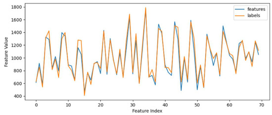
Figure 4.
FFT feature extraction of EEG signals.
2.5. ECA Module
In recent years, channel attention mechanisms have demonstrated great potential in enhancing the performance of neural networks. The ECA (Efficient Channel Attention) module is inspired by the SE (Squeeze-and-Excitation) attention module [33] and the CBAM (Convolutional Block Attention Module) [34], which offer an efficient channel attention mechanism while maintaining computational efficiency. EEG signals are commonly divided into five frequency bands: delta (1–3 Hz), theta (4–7 Hz), alpha (8–13 Hz), beta (14–29 Hz), and gamma (30–47 Hz) [35]. Research has shown that the beta and gamma bands of EEG signals exhibit the strongest response to emotions, followed by the alpha band, while the theta band shows the weakest response [36,37]. Based on this characteristic, the ECA module assigns different weights to these frequency bands, focusing on the frequency bands most relevant to emotional responses in the emotion classification task, thereby improving classification performance.
The structure of the ECA module is shown in Figure 5. Let the input feature map be ∈Rℎ×w×c, where h, w, and c represent the height, width, and number of channels, respectively. First, global average pooling (GAP) is applied along the spatial dimensions to obtain a 1 × 1 × C feature map, where C represents the number of channels. By aggregating spatial information through global average pooling, global features are extracted, which simplifies computational complexity while preserving the overall information of the input feature map. The calculation for the feature weights is as follows:
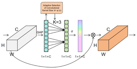
Figure 5.
ECA attention mechanism module.
The core idea of the ECA attention mechanism is to use a window function to perform a weighted summation over each channel of the feature map, calculating the weight for each channel. This helps effectively capture the interaction between channels and prevents the loss of channel information. This window function can be a one-dimensional convolutional kernel. As shown in Figure 5, local cross-channel interactions are captured through 1D convolution without reducing dimensions, where k determines the range of interaction. Since k is related to the channel dimension c, larger channel sizes result in stronger long-range interactions, while smaller channel sizes lead to stronger short-range interactions. Therefore, the following adaptive method is used to determine the kernel size:
In Equation (12), γ and b are constants, and a denotes the closest odd integer. In this study, the number of input channels C is set to 3, with both γ and b set to 1. Finally, after passing through the Sigmoid function (denoted by σ in Figure 3), the channel attention feature map is obtained. This feature map is then element-wise multiplied with the original input feature map to produce the final output feature map with channel attention.
2.6. ECA-ResDNN Model
In traditional residual networks, a max pooling layer is often added after each residual block to reduce computational cost and model complexity while retaining significant features. However, frequent pooling may cause information loss, impacting performance and generalization. To address this, we add a max pooling layer only after the final convolutional layer. As illustrated in Figure 6, the ECA-ResNet model consists of convolutional layers, batch normalization layers, three attention mechanism residual blocks, a max pooling layer, and a flatten layer.
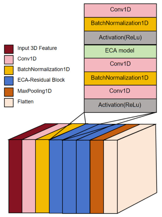
Figure 6.
ECA-ResNet model.
The parameter configuration for each attention mechanism residual block is summarized in Table 1. Each residual block includes convolutional layers, batch normalization layers, ReLU activation layers, and an ECA module. By setting the first dimension of the output shape to “None”, the model can accommodate batch data of varying sizes during training, which enhances its flexibility and generalizability. The mathematical formulation for the attention mechanism residual block is as follows:

Table 1.
Parameters of the ECA Residual Block.
In Equation (13), represents the output after convolution, batch normalization, ReLU activation, and ECA attention mechanisms. Here, x is the input feature map, and y is the output feature map after applying the residual learning.
To effectively capture both temporal and spectral features from EEG signals and achieve accurate emotion classification, this paper introduces the ECA-ResDNN (Efficient Channel Attention Residual Deep Neural Network) model. This model integrates attention mechanisms, residual networks, and deep neural networks, allowing it to deeply mine the intrinsic features of EEG signals.
As shown in Figure 7, the model consists of four main components:
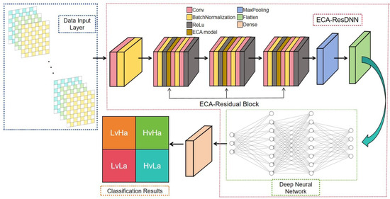
Figure 7.
ECA-ResDNN model.
- (1)
- Data Input Layer: Accepts a preprocessed three-dimensional feature matrix from various EEG signal channels.
- (2)
- Spectral Feature Extraction Layer: The ECA-ResNet model with an attention mechanism captures significant spectral information from each time slice.
- (3)
- Temporal Feature Extraction Layer: A deep neural network extracts temporal features from the ECA-ResNet output, enabling higher-level abstraction.
- (4)
- Fully Connected Layer: Final classification using a softmax activation function to categorize the input into emotional states.
3. Experimental Design
3.1. Experimental Parameter Settings
The experiments in this study were conducted using a consistent software and hardware environment. The experimental setup was performed on an HP laptop (Compal, Hangzhou, China) equipped with the TensorFlow 2.10.0 framework, an NVIDIA GeForce RTX 2080 Super graphics card (NVIDIA Corporation, Santa Clara, CA, USA), and an Intel® Core™ i7-10750H CPU (Intel Corporation, Chengdu, China). The entire training process took approximately 36 h and was distributed over a two-week period.
After preprocessing and feature extraction, the dataset was split into training and testing sets based on a specific indexing rule. One out of every eight rows was selected as the test set, with the remaining rows used as the training set. This data partitioning method was applied uniformly across all experiments to ensure consistency. Additionally, to handle outliers in the labels, any label with a value of 9 was replaced with 8.99.
For the training sessions, the batch size was set to 256. The number of epochs was configured to 120 for binary classification and 240 for eight-class classification tasks. The log display mode (verbose) was set to 1, allowing for progress updates during training.
3.2. Loss Function
This study introduces a novel loss function that integrates cross-entropy loss and fuzzy set loss, aiming to synergize the advantages of both methods for enhanced performance. The cross-entropy loss is effective for classification tasks, while the fuzzy set loss helps address uncertainty and noise in the data. The combined loss function is defined as follows:
In Equation (14), represents the cross-entropy loss, represents the fuzzy set loss, and λ is a hyperparameter in the range [0, 1] used to adjust the relative weight between the two loss functions.
The cross-entropy loss, , measures the difference between the predicted probability distribution and the true labels. Its mathematical expression is given by the following, where C is the number of classes, is the one-hot encoded true label, and is the predicted probability for the i-th class:
The fuzzy set loss, , introduces a fuzziness parameter α to control the sensitivity of the loss function to misclassifications. Its expression is as follows:
In Equation (16), α is a positive parameter that adjusts the degree of fuzziness in the loss function, allowing it to better handle uncertainty and noise in the data.
4. Result Analysis
4.1. Comparative Experiments
To comprehensively evaluate the performance and effectiveness of the proposed model, we conducted comparative experiments against four baseline models: CNN, CNN-GRU, CNN-LSTM, and DNN. These models were assessed based on their performance in EEG-based emotion classification tasks. Additionally, we compared our approach with state-of-the-art methods in emotion classification, including SPD + SVM [25] and GLFANet [26]. To ensure fairness, all experimental conditions were kept consistent except for the model architectures. Figure 8 presents the classification accuracy of the models, while Table 2 and Table 3 summarize the results for binary classification and multi-class classification tasks, respectively.
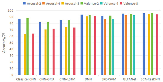
Figure 8.
Classification accuracy rates of different models.
Table 2.
Comparative model classification report (binary classification).
Table 3.
Comparative model classification report (multi-class classification).
4.1.1. Binary Classification Results
The classical CNN model achieved an accuracy of 87.68% for binary classification. The CNN-GRU model, due to the simplicity of its GRU structure, achieved an accuracy of 85.42% in binary classification. The CNN-LSTM model, capable of capturing long-term dependencies, showed moderate performance with an accuracy of 85.42% in binary classification. Lastly, the DNN model outperformed other baseline models in binary classification, achieving an accuracy of 93.15%, showcasing its strong generalization ability. In addition to the classical methods, new methods such as SPD + SVM [25] and GLFANet [26] were introduced. Among them, SPD + SVM achieved an accuracy of 91.84% for binary classification, demonstrating its ability to handle more complex feature spaces. GLFANet, which integrates global-to-local feature aggregation, reached an accuracy of 94.72%.
4.1.2. Multi-Class Classification Results
The multi-class classification task introduces more challenges, which require models to address the complex decision boundaries between multiple classes. The classical CNN model exhibits limited performance, with an accuracy of 63.80% in the eight-class classification task, reflecting its difficulty in handling multi-class scenarios. The CNN-GRU and CNN-LSTM models perform better than the CNN, leveraging their ability to model temporal dependencies, achieving accuracies of 73.72% and 71.00%, respectively. However, the DNN model achieved the best performance with an accuracy of 91.26%, effectively handling the complex features required for emotion classification across multiple categories. Moreover, SPD + SVM [25] and GLFANet [26] achieved accuracies of 86.71% and 92.92% on the four-class classification task, respectively.
4.1.3. Comparative Analysis
For the binary classification task, the CNN model demonstrated high precision, recall, and F1 scores. However, due to the adaptability of the GRU and LSTM modules for simpler tasks, their performance was relatively poor. In the eight-class classification task, which requires handling complex multi-class decision boundaries, the CNN model performed the worst. The CNN-GRU and CNN-LSTM models showed better performance in the eight-class classification. The DNN model performed the best in the eight-class task, effectively handling multi-class tasks.
The SPD + SVM model excels in handling more complex decision boundaries. By combining Spectral Power Density (SPD) features from EEG data, Support Vector Machines can effectively capture relevant information for both binary and four-class classification tasks. The high accuracy of the GLFANet model is attributed to its ability to perform global-to-local feature aggregation. Particularly in tasks with diverse and rich data, GLFANet significantly improves classification performance.
4.2. Experimental Results Analysis
This study utilized the ECA-ResDNN network model to perform binary and eight-class classification experiments on the arousal and valence dimensions of the DEAP dataset. The confusion matrices for the binary and eight-class classification tasks using the ECA-ResDNN model are depicted in Figure 9 and Figure 10, respectively. These results indicate that the model achieves high classification accuracy for both tasks. Specifically, in the binary classification task, the model performs optimally when predicting samples labeled as “1”. For the eight-class classification task, the model exhibits superior performance in predicting samples labeled as “2”, “6”, and other specific classes.
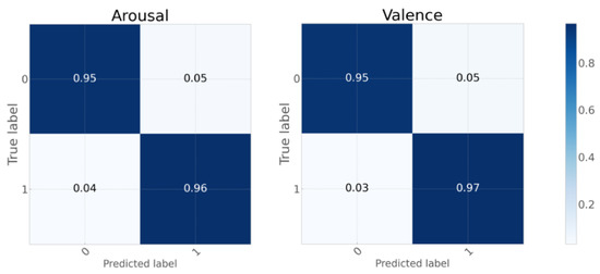
Figure 9.
Confusion matrix (binary classification).
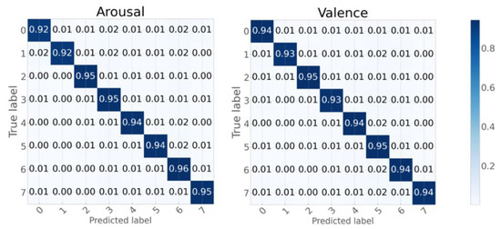
Figure 10.
Confusion matrix (eight-class classification).
Detailed statistical metrics derived from the confusion matrices are presented in Table 4 and Table 5. For the binary classification task, the average precision, recall, and F1 score of the model are all 0.96. In the eight-class classification task, the average precision, recall, and F1 score are 0.95, 0.93, and 0.94, respectively. These results demonstrate that the precision and recall values are consistently high across both tasks, leading to robust F1 scores. Furthermore, these metrics surpass those of the comparative models discussed in Section 4.1, underscoring the superior performance of the ECA-ResDNN model. The model not only excels in binary classification tasks but also maintains consistent and reliable performance in the more complex eight-class classification tasks, highlighting its robustness and generalization capabilities across varying levels of task complexity.
Table 4.
Classification report (binary classification).
Table 5.
Classification report (eight-class classification).
Table 6 presents a comparative analysis of the proposed model against other experimental models. The ECA-ResDNN network demonstrates significant performance improvements in both the arousal and valence dimensions. Specifically, it achieves classification accuracies of 95.95%, 94.33%, 96.10%, and 94.04% in binary and eight-class classification tasks, respectively. It not only outperforms other models in the binary classification task but also achieves performance in the more challenging eight-class classification task. This performance is comparable to or even surpasses that of other models in four-class tasks. Moreover, in the binary classification task, the model performs slightly better on the valence dimension than on arousal, indicating its superior ability to distinguish positive and negative emotions over capturing emotional intensity. This is because valence is closely related to asymmetric activity in the prefrontal cortex, which depends on spatial distribution, while the ECA-ResNet module enhances spatial and spectral feature extraction, improving classification performance in the valence dimension. In the eight-class classification task, the performance gap between the two dimensions becomes less significant. This is due to the deep neural network extracting higher-level temporal and global features, reducing reliance on individual spatial or spectral patterns. Additionally, the hybrid loss function enhances robustness against uncertainty and label noise, ensuring stable generalization across different emotion intensities and valence levels, thereby minimizing performance differences between the dimensions.
Table 6.
Emotional recognition results of different models.
4.3. Ablation Study
To evaluate the impact of various modules on the model’s performance and assess their contributions to performance enhancement, an ablation study was conducted on the ECA-ResDNN model. By systematically removing or replacing key components, the study examined the resulting changes in performance on the eight-class classification task. The ablation study results are summarized in Table 7, where “−ECA” indicates the removal of the ECA attention module, “+SE” and “+CBAM” represent replacing the ECA attention module with the Squeeze-and-Excitation (SE) and Convolutional Block Attention Module (CBAM) mechanisms, “−ResBlock” represents a reduction in the number of residual blocks incorporating the attention mechanism (with the parameter num_res_blocks reduced from 3 to 1), and “−” denotes the removal of the fuzzy set loss component from the combined loss function.
Table 7.
Comparison of ablation study results.
Based on the results in Table 7, the following conclusions can be drawn:
- The ECA attention module positively impacts the model’s performance, although it is not the sole determinant of success. Additionally, CBAM, which integrates both spatial and channel attention, slightly outperforms SE, indicating that spatial attention contributes to performance improvement.
- The ResBlock is critical to the model’s effectiveness. By increasing the network’s depth and complexity, ResBlock enables the capture of more comprehensive feature information, thereby significantly enhancing the model’s performance.
- Removing results in a slight performance drop, particularly in recall, suggesting that the fuzzy set loss improves classification stability by mitigating the impact of label noise and uncertainty in EEG data.
4.4. Analysis of Model Complexity
To analyze the computational burden, we present a comparative analysis of different models in terms of Model Size (KB), Running Time (seconds), FLOPs (Giga), and Parameters. As shown in Table 8, “DNN” refers to the classical DNN model without the ECA attention module and residual blocks; “−ECA” indicates the removal of the ECA attention module, and “−ResBlock” represents a reduction in the number of residual blocks that incorporate the attention mechanism (with the parameter num_res_blocks reduced from 3 to 1). According to the experimental results, it is evident that by introducing the ECA attention module and residual networks (ResNet), the model complexity increases, and the training time significantly rises. In particular, the introduction of residual blocks results in increased computation as the network depth grows, and each convolutional layer has its own set of weight matrices, which further increases the parameter count. However, this added complexity enhances the accuracy and stability of the emotion recognition task, especially in more complex multi-class classification tasks, making the increase in complexity worthwhile.
Table 8.
Comparison of model complexity results.
5. Conclusions
In this paper, we proposed a novel hybrid model, ECA-ResDNN, for EEG-based emotion recognition, aiming to address key challenges such as noise, artifacts, and signal distortions in EEG data. By integrating an advanced preprocessing method that combines Generative Adversarial Networks (GANs) and fuzzy set theory, the clarity and stability of EEG signals were significantly enhanced. The adoption of a Deep Neural Network in conjunction with an attention mechanism allowed the model to more effectively capture and represent emotional features within EEG data. Furthermore, the introduction of a hybrid loss function, which combines cross-entropy loss with fuzzy set loss, optimized the training process, thus improving the model’s sensitivity to misclassification and enhancing its generalization capabilities.
Experimental comparisons demonstrated that the proposed ECA-ResDNN model outperforms existing models in both accuracy and robustness for emotion recognition tasks. These results validate the effectiveness and reliability of our approach, suggesting promising applications in fields such as affective computing, mental health monitoring, and human–computer interaction.
In future work, we plan to explore further enhancements through multimodal fusion and the implementation of real-time systems, which will enable deployment in practical, real-world scenarios. Additionally, current source density (CSD) transformation offers a more localized representation of cortical activity by reducing volume conduction effects, thereby improving source localization and neural activity decomposition. Given its potential to enhance EEG feature extraction, we will investigate its applicability to emotion recognition and conduct comparative analyses with conventional referencing techniques.
Author Contributions
Conceptualization, J.L. and N.F.; methodology, J.L. and N.F.; software, J.L.; validation, J.L. and N.F.; formal analysis, J.L. and N.F.; investigation, J.L.; resources, Y.L.; data curation, J.L.; writing—original draft preparation, J.L.; writing—review and editing, N.F.; visualization, J.L.; supervision, Y.L.; project administration, Y.L.; funding acquisition, N.F. All authors have read and agreed to the published version of the manuscript.
Funding
This research was funded by China Postdoctoral Science Foundation (grant number 2023M732107) and Qingdao Postdoctoral Foundation (grant number QDBSH20220202177).
Data Availability Statement
Data will be made available on request.
Conflicts of Interest
The authors declare no conflicts of interest.
References
- Koelstra, S.; Muhl, C.; Soleymani, M.; Lee, J.-S.; Yazdani, A.; Ebrahimi, T.; Pun, T.; Nijholt, A.; Patras, I. Deap: A database for emotion analysis; using physiological signals. IEEE Trans. Affect. Comput. 2011, 3, 18–31. [Google Scholar] [CrossRef]
- Bhattacharya, S. Artificial intelligence, human intelligence, and the future of public health. AIMS Public Health 2022, 9, 644. [Google Scholar] [CrossRef] [PubMed]
- Xu, F.F.; Pan, D.; Zheng, H.; Ouyang, Y.; Jia, Z.; Zeng, H. EESCN: A novel spiking neural network method forEEG-based emotion recognition. Comput. Methods Programs Biomed. 2024, 243, 107927. [Google Scholar]
- Li, Y.; Wang, D.; Liu, F. The auto-correlation function aided sparse support matrix machine for EEG-based fatigue detection. IEEE Trans. Circuits Syst. II Express Briefs 2022, 70, 836–840. [Google Scholar]
- Mohsen, S.; Alharbi, A.G. EEG-based human emotion prediction using an LSTM model. In Proceedings of the 2021 IEEE International Midwest Symposium on Circuits and Systems (MWSCAS), Lansing, MI, USA, 9–11 August 2021; IEEE: Piscataway, NJ, USA, 2021; pp. 458–461. [Google Scholar]
- Du, X.; Ma, C.; Zhang, G.; Li, J.; Lai, Y.-K.; Zhao, G.; Deng, X.; Liu, Y.-J.; Wang, H. An efficient LSTM network for emotion recognition from multichannel EEG signals. IEEE Trans. Affect. Comput. 2020, 13, 1528–1540. [Google Scholar]
- Zheng, Y.; Ding, J.; Liu, F.; Wang, D. Adaptive neural decision tree for EEG based emotion recognition. Inf. Sci. 2023, 643, 119160. [Google Scholar]
- Ouyang, D.; Yuan, Y.; Li, G.; Guo, Z. The effect of time window length on EEG-based emotion recognition. Sensors 2022, 22, 4939. [Google Scholar] [CrossRef]
- Zhang, Y.; Cui, C.; Zhong, S. EEG-Based Emotion Recognition via Knowledge-Integrated Interpretable Method. Mathematics 2023, 11, 1424. [Google Scholar] [CrossRef]
- Atkinson, J.; Campos, D. Improving BCI-based emotion recognition by combining EEG feature selection and kernel classifiers. Expert Syst. Appl. 2016, 47, 35–41. [Google Scholar]
- Xing, X.; Li, Z.; Xu, T.; Shu, L.; Hu, B.; Xu, X. SAE+ LSTM: A new framework for emotion recognition from multi-channel EEG. Front. Neurorobot. 2019, 13, 37. [Google Scholar]
- Zhang, X.; Hu, B.; Chen, J.; Moore, P. Ontology-based context modeling for emotion recognition in an intelligent web. World Wide Web 2013, 16, 497–513. [Google Scholar]
- Rozgić, V.; Vitaladevuni, S.N.; Prasad, R. Robust EEG emotion classification using segment level decision fusion. In Proceedings of the 2013 IEEE International Conference on Acoustics, Speech and Signal Processing, Vancouver, BC, Canada, 26–31 May 2013; IEEE: Piscataway, NJ, USA, 2013; pp. 1286–1290. [Google Scholar]
- Yoon, H.J.; Chung, S.Y. EEG-based emotion estimation using Bayesian weighted-log-posterior function and perceptron convergence algorithm. Comput. Biol. Med. 2013, 43, 2230–2237. [Google Scholar]
- Zheng, W.L.; Zhu, J.Y.; Lu, B.L. Identifying stable patterns over time for emotion recognition from EEG. IEEE Trans. Affect. Comput. 2017, 10, 417–429. [Google Scholar] [CrossRef]
- Rayatdoost, S.; Soleymani, M. Cross-corpus EEG-based emotion recognition. In Proceedings of the 2018 IEEE 28th International Workshop on Machine Learning for Signal Processing (MLSP), Aalborg, Denmark, 17–20 September 2018; IEEE: Piscataway, NJ, USA, 2018; pp. 1–6. [Google Scholar]
- Tripathi, S.; Acharya, S.; Sharma, R.; Mittal, S.; Bhattacharya, S. Using deep and convolutional neural networks for accurate emotion classification on DEAP data. In Proceedings of the AAAI Conference on Artificial Intelligence, San Francisco, CA, USA, 4–9 February 2017; Volume 31, pp. 4746–4752. [Google Scholar]
- Chung, S.Y.; Yoon, H.J. Affective classification using Bayesian classifier and supervised learning. In Proceedings of the 2012 12th International Conference on Control, Automation and Systems, Jeju, Republic of Korea, 17–21 October 2012; IEEE: Piscataway, NJ, USA, 2012; pp. 1768–1771. [Google Scholar]
- Al-Nafjan, A.; Hosny, M.; Al-Wabil, A.; Al-Ohali, Y. Classification of human emotions from electroencephalogram (EEG) signal using deep neural network. Int. J. Adv. Comput. Sci. Appl. 2017, 8, 419–425. [Google Scholar]
- Itti, L.; Koch, C.; Niebur, E. A model of saliency-based visual attention for rapid scene analysis. IEEE Trans. Pattern Anal. Mach. Intell. 1998, 20, 1254–1259. [Google Scholar]
- Liu, S.; Wang, X.; Zhao, L.; Li, B.; Hu, W.; Yu, J.; Zhang, Y. 3DCANN: A spatio-temporal convolution attention neural network for EEG emotion recognition. IEEE J. Biomed. Health Inform. 2021, 26, 5321–5331. [Google Scholar]
- Tao, W.; Li, C.; Song, R.; Cheng, J.; Liu, Y.; Wan, F.; Chen, X. EEG-based emotion recognition via channel-wise attention and self attention. IEEE Trans. Affect. Comput. 2020, 14, 382–393. [Google Scholar]
- Zhang, Y.; Liu, H.; Zhang, D.; Chen, X.; Qin, T.; Zheng, Q. EEG-based emotion recognition with emotion localization via hierarchical self-attention. IEEE Trans. Affect. Comput. 2022, 14, 2458–2469. [Google Scholar]
- Liu, J.; Wu, H.; Zhang, L.; Zhao, Y. Spatial-temporal transformers for EEG emotion recognition. In Proceedings of the 6th International Conference on Advances in Artificial Intelligence, New York, NY, USA, 21–23 October 2022; pp. 116–120. [Google Scholar]
- Gao, Y.; Sun, X.; Meng, M.; Zhang, Y. EEG emotion recognition based on enhanced SPD matrix and manifold dimensionality reduction. Comput. Biol. Med. 2022, 146, 105606. [Google Scholar]
- Liu, S.; Zhao, Y.; An, Y.; Zhao, J.; Wang, S.-H.; Yan, J. GLFANet: A global to local feature aggregation network for EEG emotion recognition. Biomed. Signal Process. Control 2023, 85, 104799. [Google Scholar]
- Lebedev, M.A.; Nicolelis, M.A.L. Brain–machine interfaces: Past, present and future. Trends Neurosci. 2006, 29, 536–546. [Google Scholar] [CrossRef] [PubMed]
- Arjovsky, M.; Chintala, S.; Bottou, L. Wasserstein generative adversarial networks. In Proceedings of the International Conference on Machine Learning, PMLR, Sydney, Australia, 6–11 August 2017; pp. 214–223. [Google Scholar]
- Goodfellow, I.; Pouget-Abadie, J.; Mirza, M.; Xu, B.; Warde-Farley, D.; Ozair, S.; Courville, A.; Bengio, Y. Generative adversarial nets. Adv. Neural Inf. Process. Syst. 2014, 27. [Google Scholar]
- Zhang, R.; Zeng, Y.; Tong, L.; Shu, J.; Lu, R.; Yang, K.; Li, Z.; Yan, B. Erp-wgan: A data augmentation method for EEG single-trial detection. J. Neurosci. Methods 2022, 376, 109621. [Google Scholar] [CrossRef] [PubMed]
- Bezdek, J.C.; Ehrlich, R.; Full, W. FCM: The fuzzy c-means clustering algorithm. Comput. Geosci. 1984, 10, 191–203. [Google Scholar] [CrossRef]
- Gonzales, R.C.; Wintz, P. Digital Image Processing; Addison-Wesley Longman Publishing Co., Inc.: Boston, MA, USA, 1987. [Google Scholar]
- Hu, J.; Shen, L.; Sun, G. Squeeze-and-excitation networks. In Proceedings of the IEEE Conference on Computer Vision and Pattern Recognition, Salt Lake City, UT, USA, 18–23 June 2018; pp. 7132–7141. [Google Scholar]
- Woo, S.; Park, J.; Lee, J.Y.; Kweon, I.S. Cbam: Convolutional block attention module. In Proceedings of the European Conference on Computer Vision (ECCV), Munich, Germany, 8–14 September 2018; pp. 3–19. [Google Scholar]
- Ray, W.J.; Cole, H.W. EEG alpha activity reflects attentional demands, and beta activity reflects emotional and cognitive processes. Science 1985, 228, 750–752. [Google Scholar] [CrossRef]
- Barry, R.J.; Clarke, A.R.; Johnstone, S.J.; Brown, C.R. EEG differences in children between eyes-closed and eyes-open resting conditions. Clin. Neurophysiol. 2009, 120, 1806–1811. [Google Scholar] [CrossRef]
- Onton, J.A.; Makeig, S. High-frequency broadband modulation of electroencephalographic spectra. Front. Hum. Neurosci. 2009, 3, 560. [Google Scholar] [CrossRef]
Disclaimer/Publisher’s Note: The statements, opinions and data contained in all publications are solely those of the individual author(s) and contributor(s) and not of MDPI and/or the editor(s). MDPI and/or the editor(s) disclaim responsibility for any injury to people or property resulting from any ideas, methods, instructions or products referred to in the content. |
© 2025 by the authors. Licensee MDPI, Basel, Switzerland. This article is an open access article distributed under the terms and conditions of the Creative Commons Attribution (CC BY) license (https://creativecommons.org/licenses/by/4.0/).