Abstract
Motivated by important biophysical applications, we study the stochastic version of a mathematical model of calcium oscillations. For the deterministic model proposed by Li and Rinzel, a parametric zone of tristability, where two stable equilibria and a limit cycle coexist, is found for the first time. In this zone, and also in adjacent bi- and monostability zones, different scenarios of noise-induced generation and suppression of complex calcium oscillations are studied in detail. In these studies, along with the traditional direct numerical simulation and statistical processing, a new analytical apparatus of the stochastic sensitivity technique and confidence domains is effectively used.
Keywords:
mathematical modelling; calcium oscillations; multistability; stochastic sensitivity; confidence domains; stochastic preference MSC:
37H10; 37H20
1. Introduction
Intracellular calcium dynamics and its exchange processes during intercellular interactions are fundamental to the information processing mechanisms that enable living organisms to sense and respond to environmental stimuli. In many cell types, exposure to external signals leads not only to a sharp increase in calcium ion concentration but also to an oscillatory behaviour [1,2,3,4]. Understanding the mathematical basis of these calcium oscillations and identifying their driving mechanisms represent key challenges for modern biophysics [5,6,7,8,9,10]. Here, in particular, mathematical models based on the fractional advection–diffusion equations for cellular calcium are studied (see, e.g., [11,12] and bibliography therein).
As studies have shown, the relationships that determine calcium dynamics are highly nonlinear. It is well known that under conditions of strong nonlinearity, mathematical models can demonstrate multistability [13], i.e., the coexistence of several, often qualitatively different, dynamic regimes. Then, the dynamics of the system depends not only on the model parameters but also on the choice of initial data. In multistable systems, random perturbations cause transitions between coexisting attractors, which significantly complicates the dynamics scenarios and generates oscillatory regimes that have no analogues in the original deterministic models [14,15,16,17,18,19]. Therefore, identifying multistability modes in calcium dynamics models is fundamental to understanding the variety of possible oscillatory modes induced by random perturbations. The study of stochastic calcium oscillations is the subject of active research (see, e.g., [20,21,22,23,24]).
In this paper, the conceptual deterministic model of calcium dynamics proposed by Li and Rinzel in [25] is considered as a baseline. This model, which is a simplification of the two-variable De Young-Kaiser model [26], captures the main features of calcium oscillations (see biophysical details in [25]). In [27], different types of calcium oscillations in the deterministic Li–Rinzel model were characterized by different encoding of external stimuli in amplitude and frequency modulation. This model was studied in many papers (see, e.g., [7,28] and bibliography therein) where mono- and bistability modes were parametrically described.
In this paper, for the first time, a parametric zone of tristability with the coexistence of two stable equilibria and a limit cycle is found. This tristability is the reason for the complexity of the dependence of calcium dynamics on the initial data. Thus, depending on the initial data, calcium concentration can either stabilize to two different equilibrium regimes or make calcium self-oscillations of large amplitudes. Section 2 presents the results of a bifurcation analysis and describes the dynamical regimes in this tristable zone and in the adjacent zones with bi- and monostability.
The aim of this work is to investigate the response of cells to the inevitably present random perturbations of calcium flux through inositol triphosphate channels in a system with such a high number of coexisting attractors. Section 3 introduces a stochastic model that accounts for random fluctuations in the parameter that determines the calcium flux intensity. Our further study of stochastic effects is based on direct numerical modelling of stochastic system solutions [29,30] and the new mathematical apparatus of stochastic sensitivity function and confidence domains [31,32,33,34]. We study conditions under which random perturbations transfer the system from the equilibrium regimes to the oscillatory modes and vice versa, generating both unidirectional transitions and bidirectional ones with the formation of complex mixed-mode oscillations.
2. Deterministic Model
Consider the Li–Rinzel model [25,35] of calcium oscillations:
The dynamical variables of the Li–Rinzel model (1) are the free cytosolic concentration c and the fraction h of the open inositol trisphosphate receptor subunits.
The dynamics of the calcium concentration c is governed by three fluxes: a passive leak of from the endoplasmic reticulum to the cytosol, ; an active uptake of into the endoplasmic reticulum due to the action of the pumps, ; a release, , that is mutually gated by and the inositol trisphosphate concentration p.
Here, we follow [27] in notations and choice of fix values of parameters as follows:
In this paper, we considered = 0.04 M and used the inositol trisphosphate concentration p as a key bifurcation parameter. The value of p changes under the signals entering the cell from the external environment, which in turn affects the dynamics of calcium concentration. Mathematically, qualitative changes in calcium dynamics are described by the bifurcation diagram and enlarged fragment shown in Figure 1a,b. Here, six bifurcation points are marked: and In this diagram, we plotted the c-coordinates of equilibria and extreme values of cycles . Stable equilibria are shown with solid lines, and unstable equilibria are shown with dashed lines.
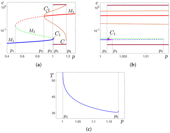
Figure 1.
Deterministic system (1): (a) bifurcation diagram; (b) the enlarged fragment with tristability zone ; (c) period of limit cycles. In the bifurcation diagram, values are = 0.50933, = 0.88385, = 1.00147, = 1.00266, = 1.01385, and = 1.18042. In (a,b), we show stable equilibria (solid, blue), (solid, red), unstable equilibria (dashed, blue), (dashed, red), (dashed, green), stable cycle C (brown), unstable cycle (magenta), and unstable cycle (light brown).
The equilibrium (blue) is stable in the interval and unstable for . The equilibrium (red) is stable in the interval and unstable for . The unstable equilibrium (green) exists for . The stable cycle C (brown) exists for . The unstable cycle (magenta) surrounding the stable equilibrium is observed in the interval . The unstable cycle (light brown) surrounding the stable equilibrium is observed in the interval .
The system (1) models an important class of calcium oscillations with frequency modulation. Indeed, in system (1), a period of the self-oscillations significantly depends on the parameter p (see Figure 1c).
Several phase portraits illustrating zones of tri-, bi-, and monostability are plotted in Figure 2. The tristability zone is presented in Figure 2a for . Here, we show stable equilibria (blue dot), (red dot), the unstable equilibrium (empty green circle), the stable cycle C (brown), the unstable cycle (magenta), and the unstable cycle (light brown). Unstable cycles play an important role by separating basins of coexisting attractors , and C. The bistability zone is presented in Figure 2b for . Here, we show the stable equilibrium (red dot), the stable cycle C (brown), and the unstable cycle (light brown) which separates basins of and C. A phase portrait for the monostability zone is presented in Figure 2c for , where the stable equilibrium (red dot) and a phase trajectory (black) are plotted.
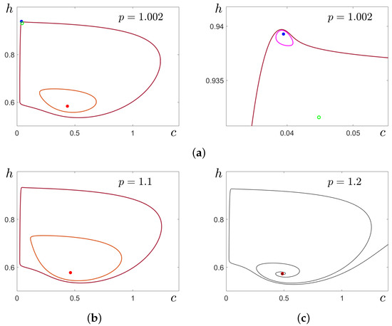
Figure 2.
Phase portraits of the deterministic system (1) for (a) , (b) , (c) . Here, we show stable equilibria (blue dot), (red dot), unstable equilibrium (green empty circle), stable cycle C (brown), unstable cycle (magenta), and unstable cycle (light brown).
Because of high nonlinearity and multistability of system (1), random disturbances can generate a wide variety of calcium oscillatory regimes.
3. Stochastic Model
In this paper, we considered the following stochastic version of the model
accounting for parametric random disturbances in the flux : Here, is a white Gaussian noise of intensity . Thus, in system (2), we have
Under stochastic perturbations, the random solutions of system (2) leave the attractors from which they started and form some probability distribution. For weak noise, random solutions are localised near the initial deterministic attractors. In Figure 3, for , = 0.02, we show in green system (2) solutions starting at the equilibrium (red dot) and the cycle C (brown). As can be seen, in both cases, the dispersion of random solutions is quite non-uniform. For a quantitative description of this dispersion, we apply the stochastic sensitivity technique [28,31].
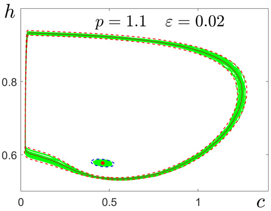
Figure 3.
Random solutions (green) of the stochastic system (2) with , confidence ellipse around the equilibrium (red dot), and confidence band around the cycle C (brown).
3.1. Stochastic Sensitivity of Attractors
In understanding the internal mechanisms of the various noise-induced deformations of calcium oscillations, a stochastic sensitivity analysis of the coexisting attractors plays an important role.
Stochastic sensitivity theory was initiated by studies on the quasipotential approximation of nonlinear stochastic differential equations. Under the influence of random perturbations, around the attractors of the system, a probability distribution is formed, the geometrical properties of which are determined by the spectral characteristics of the corresponding stochastic sensitivity matrix. Using these spectral characteristics, one can construct a confidence domain around the attractor that approximates the dispersion of the random states: an ellipsoid around the equilibrium and a torus around the cycle [36]. For discrete-time systems, the theory of stochastic sensitivity has been developed for the cases of quasiperiodic and chaotic attractors (see, e.g., [37]). This theory and the confidence domain method have been successfully applied to studies of the constructive role of noise in mathematical models of neural activity [32,38], population dynamics [34,39], climatology [33], pattern formation [40], etc.
Let us briefly discuss the stochastic sensitivity technique for equilibria and cycles of the two-dimensional continuous-time model (2) of calcium stochastic dynamics. In this case, the stochastic sensitivity of the stable equilibrium is determined by the -matrix W, which is a unique solution of the matrix equation
due to the stability of the equilibrium. Here, F is the Jacobi matrix of the initial deterministic system at point M, and G is the matrix characterizing random disturbances. For system (2), matrix G is written as
Let be eigenvalues and be normalized eigenvectors of the stochastic sensitivity matrix W. The geometrical arrangement of system (2)’s random solutions around the equilibrium is described by the confidence ellipse
Here, are coordinates of this ellipse in the basis of eigenvectors of the matrix W with the point M as an origin, and is a fiducial probability. Note that eigenvalues and define the eccentricity of the confidence ellipse. In Figure 4, plots of eigenvalues of the stochastic sensitivity matrices are shown for the equilibrium (a) and the equilibrium (b). As parameter p approaches the bifurcation values and , stochastic sensitivity increases unboundedly. In Figure 3, the confidence ellipse is shown around for .
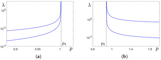
Figure 4.
Stochastic sensitivity of equilibria in system (2). Here, plots of eigenvalues of the stochastic sensitivity matrices are depicted for (a) the equilibrium and (b) the equilibrium .
The stochastic sensitivity of the T-periodic solution which determines the stable cycle C in the two-dimensional deterministic system is a solution of the boundary problem
where Here, is a normalized vector that is orthogonal to cycle C at the current point . The geometrical arrangement of system (2) random solutions around cycle C is described by the confidence band. The boundaries of this band are written as:
Characterizing the stochastic sensitivity of the cycle as a whole, we use the stochastic sensitivity factor
In Figure 5a, stochastic sensitivity function is plotted for (green), (blue), and (magenta). As can be seen, the stochastic sensitivity of cycles under consideration is highly nonuniform. In Figure 5b, the stochastic sensitivity factor is plotted versus parameter p. This function tends to infinity as parameter p approaches bifurcation values and . In Figure 3, the confidence band around the deterministic cycle C is shown for . As can be seen, this band adequately reflects non-uniformity of dispersion of random solutions along the cycle.
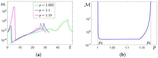
Figure 5.
Stochastic system (2): (a) stochastic sensitivity of cycles for (green), (blue), and (magenta); (b) stochastic sensitivity factor .
It should be noted that the stochastic sensitivity technique provides a quantitative description of the response of calcium oscillations to random perturbations. The confidence domain method allows one to parametrically study complex deformations of calcium dynamics in multistable systems.
3.2. Noise-Induced Effects in the Tristability Zone
Here, we consider a parametric tristability zone when the concentration p of the inositol triphosphate belongs to the range . In this zone, system (1) shows the coexistence of the stable equilibria , and the stable limit cycle C. Recall that basins of , are separated from the basin of C by orbits of unstable cycles , respectively (see Figure 1 and Figure 2). In this multistability zone, system (2) exhibits rather complex scenarios of stochastic transformations.
Let us first compare the effect of noise on the equilibrium and the limit cycle C. These attractors are very close to each other, and noise-induced transformations occur at very small noise. In Figure 6, for three values of p, we show changes in the dispersion of random states for system (2)’s solutions starting at the stable equilibrium (Figure 6a) and cycle C (Figure 6b). In Figure 6a, one can see how the regime of small-amplitude stochastic oscillations (SASOs) near abruptly transforms into the large-amplitude stochastic oscillation (LASO) mode. More complex, three-stage scenarios are shown in Figure 6b. For weak noise, random solutions starting at cycle C slightly fluctuate around it. When exceeds some threshold, random solutions leave the basin of the cycle and begin to oscillate near with small amplitudes. Such a SASO regime is observed in some window. As the noise is further increased, this mode breaks down and the system enters the LASO mode again. It should be noted that the size of the window of SASOs decreases, and this window disappears with the increase in the parameter p (see Figure 6b).
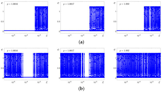
Figure 6.
Random states of stochastic system (2)’s solutions after the transient versus noise intensity . In (a), solutions start at the stable equilibrium ; in (b), at the stable limit cycle C.
In Figure 7a,b, these transformations are illustrated for by time series of stochastic solutions starting at (Figure 7a) and at cycle C (Figure 7b). Here, the results of stochastic forcing for four values of the noise intensity are compared. At , the random solutions oscillate slightly around the deterministic attractors where they started. For , this behaviour is preserved for solutions starting at , but solutions starting at C exhibit a unidirectional transition . At , for both cases, the noise induces two-way transitions , and one can see mixed-mode stochastic oscillations with alternation of SASOs near and LASOs of spike form near C. With a further increase in noise, the frequency of spikes grows (see bottom panels for ).
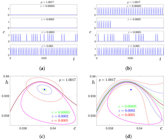
Figure 7.
Noise-induced transitions between the equilibrium and limit cycle C for . In the top panel, we show time series of stochastic solutions starting at (a) and at the cycle C (b). In the bottom panel, we show stable equilibrium (blue dot), stable cycle C (brown), and unstable cycle (magenta). In (c), confidence ellipses (dashed curves) are shown for different values of noise intensity by corresponding colors. In (d), boundaries of confidence bands (dashed curves) are shown for different values of noise intensity by corresponding colors. Here, the fiducial probability is = 0.99.
To analyse these transitions parametrically, one can apply the stochastic sensitivity technique and method of confidence domains presented in Section 3.1. In Figure 7c,d, for , an enlarged fragment of the phase plane is presented. Here, the stable equilibrium is shown by a blue dot, the stable cycle C is plotted in brown, and the unstable cycle separating the basins of these attractors is shown in magenta. For three values of noise intensity, confidence ellipses (dashed) around are shown in Figure 7c, and confidence bands (dashed) around cycle C are shown in Figure 7d by the same colours. As can be seen in Figure 7c, for and , confidence ellipses entirely belong to the basin of . This arrangement means that random trajectories starting at are located near . For , the confidence ellipse (red) crosses the separatrix and partially occupies the basin of C. It means that random trajectories with high probability fall into the basin of C and exhibit a LASO regime. As can be seen in Figure 7d, for , the confidence band lies completely in the basin of C. For , the band contains points of the basin of , while the ellipse does not intersect the separatrix. This mutual arrangement of the ellipse and the band signals unidirectional transitions , and thus, for , the “stochastic preference” [41] of the equilibrium can be stated. For , both confidence domains cross the separatrix, so two-way transitions occur, generating a mixed-type stochastic oscillation regime (see Figure 7a,b).
Results of the detailed statistical analysis of noise-induced amplitude and frequency transformations of solutions starting at the cycle C are represented in Figure 8 versus the noise intensity for four values of p which belong to the tristability parametric zone. In Figure 8a, in plots of variance , it is well seen how the windows of SASO regimes narrow and disappear with the increase in p.
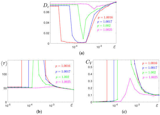
Figure 8.
Amplitude and frequency deformations of stochastic system (2) solutions starting at the stable limit cycle: (a) variance of coordinates of random states; (b) mean values of interspike intervals; (c) coefficient of variation of interspike intervals.
To analyse the frequency characteristics of complex stochastic spike oscillations, we use the statistics of interspike intervals : the mean values (Figure 8b) and the coefficient of variation Figure 8c). For weak noise, when stochastic trajectories are close to the deterministic cycle, the coefficient is almost zero, so stochastic oscillations are almost coherent. A sharp jump up and down in the plot of well localises the boundaries of the interval of the SASO regime. In the zone of the mixed-mode stochastic oscillations, for , the frequency of spikes grows with increasing (see also the time series in Figure 7b).
Let us fix and consider the effect of noise on the equilibrium and the limit cycle C. In Figure 9a, we show changes in the dispersion of random states for system (2) solutions starting at the stable equilibrium . Here, an abrupt noise-induced transition is well seen. In Figure 9b, time series of stochastic solutions starting at are plotted for three values of . For , these solutions demonstrate a SASO regime near . For , and the stochastic transition from SASO to LASO with spike oscillations is observed. For , one can see the generation of mixed-mode oscillations with alternation of spikes and oscillations near . In Figure 9c, for the same values of , oscillatory regimes are shown for solutions starting at cycle C. Here, the only transition from spike oscillations to mixed-mode oscillations is observed.
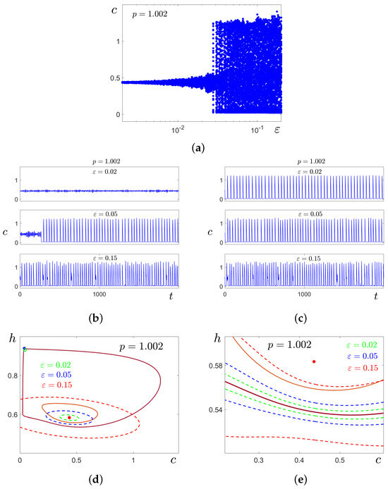
Figure 9.
Noise-induced transitions between the equilibrium and limit cycle for . In (a), random states for system (2) solutions starting at the stable equilibrium are shown. In the middle panel, we show time series of stochastic solutions starting at (b) and at the cycle C (c). In the bottom panel, we show stable equilibria (blue dot), (red dot), unstable equilibrium (empty green circle), stable cycle C (brown), and unstable cycle (light brown). In (d), confidence ellipses (dashed curves) are shown for different values of noise intensity by corresponding colors. In (e), boundaries of confidence bands (dashed curves) are shown for different values of noise intensity by corresponding colors. Here, = 0.99.
Consider how the confidence domains method works in the analysis of these transformations. In Figure 9d,e, for , the stable equilibrium is shown by a red dot, the stable cycle C is plotted in brown, and the unstable cycle separating the basins of these attractors is shown in light brown. For three values of noise intensity, confidence ellipses (dashed) around are shown in Figure 9d, and confidence bands (dashed) around the cycle C are shown against the enlarged fragment of the phase plane in Figure 9e by the same colours. For , the confidence ellipse belongs to the basin of and the confidence band entirely lies in the basin of C. Thus, noise-induced transitions between and C do not occur. For , the confidence ellipse (blue) partially occupies the basin of C while the confidence band lies within the basin of C. This geometrical arrangement signals the one-way noise-induced transition , and therefore, the “stochastic preference” of the cycle C. Recall that in the pair and C discussed above, the stochastic preference is for the equilibrium . For , both ellipses and bands partially occupy basins of opposite attractors. This signals the bidirectional stochastic transitions, and hence the formation of a mixed-mode regime (see the time series in Figure 9b,c).
The results of the statistical analysis of changes in the amplitude–frequency characteristics of stochastic system (2)’s solutions starting at the stable limit cycle (blue) and stable equilibrium (red), caused by increasing noise, are shown in Figure 10. Here, jumps in red lines mark transitions from the equilibrium to the cycle. As the noise is further increased, the distributions are mixed, and the characteristics merge.
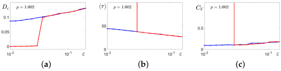
Figure 10.
Amplitude and frequency deformations of stochastic system (2)solutions starting at the stable limit cycle C (blue) and the stable equilibrium (red): (a) variance of coordinates of random states; (b) mean values of interspike intervals; (c) coefficient of variation of interspike intervals.
To summarize, in the tristability parameter zone, a wide variety of stochastic regimes is observed. For weak noise, we have the coexistence of noisy equilibrium noisy equilibrium , and noisy cycle C. Biologically, this means that depending on the initial data, calcium can either be in a noisy oscillation mode with a high concentration (near ), a low concentration (near ), or oscillate with a large amplitude of concentration change (along C).
With increasing noise, system (2) exhibits a unidirectional transition , which can be biologically interpreted as the suppression of calcium oscillations by noise, and a unidirectional transition , which can be interpreted as the generation of calcium oscillations by noise. With a further increase in noise, more complex, mixed-mode regimes with alternating large-amplitude spike oscillations and small-amplitude stochastic fluctuations near or are observed. Thus, in the tristability case, random noise can qualitatively deform the character of calcium oscillations.
3.3. Noise-Induced Effects in the Bistability Zone
Consider now the behaviour of stochastic system (2) in the bistability zone , where the stable equilibrium coexists with the limit cycle C. Their basins are separated by the orbit of the unstable cycle (see the bifurcation diagram in Figure 1 and the phase portrait in Figure 2b for , as an example).
Let us compare for this bistability zone how noise affects the equilibrium and the limit cycle C. In Figure 11, for three values of p with , we show changes in the dispersion of random states for system (2)’s solutions starting at cycle C (Figure 11a) and equilibrium (Figure 11b). Figure 8a (left) shows that for , the LASO regime is preserved when noise intensity increases. For and , one can see three-stage scenarios of stochastic transformations. For weak noise, random solutions starting at cycle C slightly fluctuate around it, demonstrating a LASO regime. When exceeds some threshold, random solutions leave the basin of cycle C and begin to oscillate near with small amplitudes. Such a SASO regime is observed in some window. With the further increase in noise, this regime breaks down, and system (2) returns to the LASO mode again. The size of this window of SASOs increases with the increase in the parameter p (see Figure 11a). In Figure 11b, one can see how the SASO regime near abruptly transforms into the LASO mode.
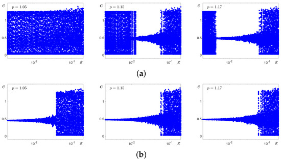
Figure 11.
Random states of stochastic system (2) solutions after the transient versus noise intensity . In (a), solutions start at the stable limit cycle C; in (b), at the stable equilibrium .
In Figure 12a,b, these transformations are illustrated for by time series of stochastic solutions starting at cycle C (Figure 12a) and equilibrium (Figure 12b). Here, we compare the results of stochastic forcing for three values of the noise intensity . At , the random solutions oscillate slightly around the deterministic attractors where they started. For , this behaviour is preserved for solutions starting at , but solutions starting at C exhibit a one-way transition . At , for both cases, noise induces two-way transitions , and one can see mixed-mode stochastic oscillations with the alternation of SASOs near and LASOs of spike form near C.
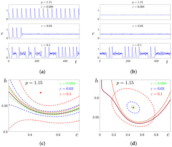
Figure 12.
Noise-induced transitions between the equilibrium and limit cycle C for . In the top panel, we show time series of stochastic solutions starting at the cycle C (a) and at the equilibrium (b). In the bottom panel, we show stable equilibrium (red dot), stable cycle C (brown), and unstable cycle (light brown). In (c), boundaries of confidence bands (dashed curves) are shown for different values of noise intensity by corresponding colors. In (d), confidence ellipses (dashed curves) are shown for different values of noise intensity by corresponding colors. Here, = 0.99.
Consider now how these stochastic transformations can be predicted analytically by the confidence domains method. In Figure 12c,d, for , the stable equilibrium is shown by the red dot, the stable cycle C is plotted in brown, and the unstable cycle separating basins of these attractors is shown in light brown. For three values of noise intensity , confidence bands (dashed) around C are shown in Figure 12c, and confidence ellipses (dashed) around the equilibrium are shown in Figure 12d by the same colours. For , the confidence band entirely lies in the basin of C, and the confidence ellipse belongs to the basin of . This means that noise-induced transitions between C and do not occur. For , the confidence band (blue) partially occupies the basin of C, while the confidence ellipse lies within the basin of . This geometrical arrangement of confidence domains and the separatrix signals the one-way noise-induced transition , and therefore, the “stochastic preference” of the equilibrium . For , both ellipses and bands capture basins of opposite attractors. This predicts the onset of bidirectional stochastic transitions, and hence the formation of a mixed-mode regime (see the time series in Figure 12a,b). Interestingly, the “stochastic preference” in the pair C and essentially depends on parameter p. Indeed, for (see Figure 9), we have noise-induced transitions , while for (see Figure 12), we have an opposite transition .
These results shed light on the intrinsic mechanisms for the formation of unexpected changes in calcium dynamics when large-amplitude oscillations of the concentration alternate with small-amplitude phases. Let us compare the statistics of the noise-induced amplitude and frequency transformations of solutions starting at cycle C for four values of parameter p lying in the bistability parametric zone. In Figure 13a, in plots of the variance , it is well seen how windows of SASO regimes appear and expand with the increase in p. In Figure 13b,c, mean values and coefficient of variation of interspike intervals are shown.
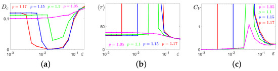
Figure 13.
Amplitude and frequency deformations of system (2) solutions starting at the stable limit cycle: (a) variance of coordinates of random states; (b) mean values of interspike intervals; (c) coefficient of variation of interspike intervals.
3.4. Stochastic Excitement in the Monostability Zone
Consider now a parametric zone where the stable equilibrium is a sole attractor of the deterministic system (1). In this case of monostability, all solutions of system (1), regardless of the initial data, converge to the point . However, the convergence character of these solutions may differ significantly. For initial values close enough to , the solutions immediately tend to . We call this set of initial data the subcritical zone. For initial values that are farther from equilibrium than some critical distance, the solutions first move away from , make a large-amplitude turn, and only then begin to tend to . We call this set of initial data the supercritical zone. Such a dichotomy is well seen in Figure 14a for , where the deterministic phase trajectory is shown in black, and equilibrium is marked by a red dot. In this figure, we plotted two confidence ellipses for stochastic system (2) with (blue) and (red). The smaller ellipse lies in the subcritical zone, so the random trajectories starting at are arranged near . This means that system (2) for is in the SASO regime. The larger ellipse captures the points of the supercritical zone, so the random trajectories can move away from , and in system (2) with , the LASO mode is observed.
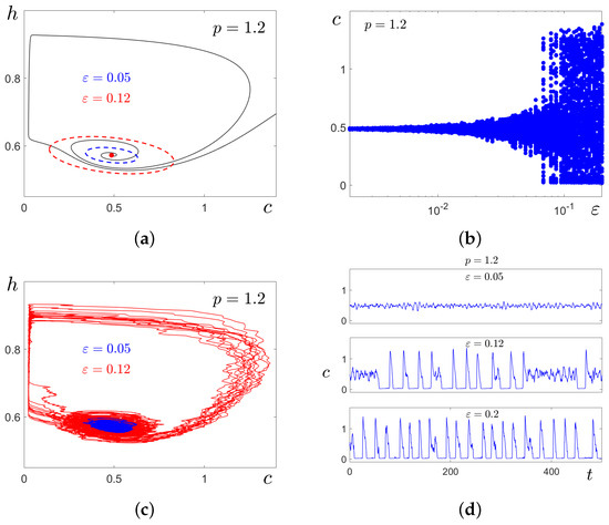
The process of transformation from the SASO regime to the LASO mode with a gradual increase in the noise intensity is shown in Figure 14b. In Figure 14c,d, regimes of SASOs and LASOs in system (2) with are illustrated by phase trajectories and time series. Note that in this case, the LASO regime is an alternation of small-amplitude fluctuations near and large-amplitude spikes (see Figure 14d). As can be seen, the prediction given by the confidence ellipses agrees well with the results of direct numerical simulations.
Details of the statistical analysis of amplitude and frequency noise-induced deformations in system (2) in the parametric monostability zone are shown in Figure 15. As can be seen in the plot of the variance in Figure 15a, the transition from SASOs to LASOs for larger p requires a stronger noise. The sharp drop in the mean values of the interspike intervals in Figure 15b localises the onset of the noise-induced excitation of the spike oscillations. Plots of the coefficient of variation in Figure 15c indicate that these spike oscillations are rather coherent.
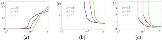
Figure 15.
Amplitude and frequency deformations of system (2) solutions starting at the stable equilibrium : (a) variance of coordinates of random states; (b) mean values of interspike intervals; (c) coefficient of variation of interspike intervals.
To summarize, even in the monostable case with the single stable equilibrium, the calcium concentration can oscillate with large amplitudes in the presence of random noise. As can be seen, the mathematical confidence domain method based on the stochastic sensitivity technique can successfully predict this important biological phenomenon.
4. Conclusions
In this paper, we studied a mathematical model describing the dynamic interaction of the free cytosolic concentration and the fraction of the open inositol trisphosphate receptor subunits. For this model, parametric zones of tri-, bi- and monostability were determined. The main content of the paper was devoted to answering the question of how the inevitably present random perturbations in calcium fluxes deformed the behaviour of the system and generated dynamic regimes that had no analogues within the deterministic consideration. In this work, noise-induced transitions for different cases of multistability were investigated in detail. The conditions under which random perturbations transferred the system from the equilibrium regime to the oscillatory regime and vice versa, generating both unidirectional transitions and bidirectional ones with the formation of complex mixed-mode oscillations, were revealed. In these studies, along with the traditional apparatus of direct numerical modelling and statistical processing, a new analytical approach using the stochastic sensitivity technique and the confidence domain method was applied. The paper shed light on the internal mechanisms of calcium oscillations and demonstrated the research potential of the new mathematical apparatus for stochastic sensitivity. The authors believe that this approach will also be useful in studying more complex calcium models of higher dimensions that take into account additional intracellular factors and intercellular connections.
Author Contributions
Conceptualization, I.B. and L.R.; methodology, I.B. and L.R.; software, I.B.; validation, I.B. and L.R.; formal analysis, I.B. and L.R.; investigation, I.B. and L.R.; writing—original draft preparation, I.B. and L.R.; writing—review and editing, I.B. and L.R.; visualization, I.B.; funding acquisition, L.R. All authors have read and agreed to the published version of the manuscript.
Funding
The work was supported by the Russian Science Foundation (N 24-11-00097).
Data Availability Statement
The original contributions presented in this study are included in the article material. Further inquiries can be directed to the corresponding authors.
Conflicts of Interest
The authors declare no conflicts of interest.
References
- Berridge, M.J. Calcium oscillations. J. Biol. Chem. 1990, 265, 9583–9586. [Google Scholar] [PubMed]
- Putney, J.W.; Bird, G.S. Cytoplasmic calcium oscillations and store-operated calcium influx. J. Physiol. 2008, 586, 3055–3059. [Google Scholar] [CrossRef] [PubMed]
- Astashev, M.E.; Serov, D.A.; Tankanag, A.V.; Knyazeva, I.V.; Dorokhov, A.A.; Simakin, A.V.; Gudkov, S.V. Study of the synchronization and transmission of intracellular signaling oscillations in cells using bispectral analysis. Biology 2024, 13, 685. [Google Scholar] [CrossRef] [PubMed]
- Rahmani, B.; Jelbart, S.; Kirk, V.; Sneyd, J. Understanding broad-spike oscillations in a model of intracellular calcium dynamics. SIAM J. Appl. Dyn. Syst. 2025, 24, 131–164. [Google Scholar] [CrossRef]
- Tsaneva-Atanasova, K. A Mathematical Study of Calcium Oscillations and Waves; VDM Verlag: Saarbrücken, Germany, 2009; p. 176. [Google Scholar]
- Dupont, G. Models of Calcium Signalling; Springer Science: New York, NY, USA, 2016. [Google Scholar]
- Shakhidzhanov, S.S.; Balabin, F.A.; Obydennyy, S.I.; Ataullakhanov, F.I.; Sveshnikova, A.N. Calcium oscillations in blood platelets and their possible role in interpreting extracellular information by cells. Phys.-Uspekhi 2019, 62, 660–674. [Google Scholar] [CrossRef]
- Tian, W.; Wang, C.; Gao, Q.; Li, L.; Luan, S. Calcium spikes, waves and oscillations in plant development and biotic interactions. Nat. Plants 2020, 6, 750–759. [Google Scholar] [CrossRef]
- Fukuoka, M.; Kang, W.; Horiike, S.; Yamada, M.; Miyado, K. Calcium oscillations and mitochondrial enzymes in stem cells. Regen. Ther. 2024, 26, 811–818. [Google Scholar] [CrossRef]
- Joshi, H.; Yavuz, M. Numerical analysis of compound biochemical calcium oscillations process in hepatocyte cells. Adv. Biol. 2024, 8, 2300647. [Google Scholar] [CrossRef]
- Bhatter, S.; Jangid, K.; Kumawat, S.; Purohit, S.D.; Baleanu, D.; Suthar, D.L. A generalized study of the distribution of buffer over calcium on a fractional dimension. Appl. Math. Sci. Eng. 2023, 31, 2217323. [Google Scholar] [CrossRef]
- Agarwal, R.; Purohit, S.D.; Kritika. Modeling Calcium Signaling: A Fractional Perspective; Springer Nature: Berlin/Heidelberg, Germany, 2024. [Google Scholar]
- Pisarchik, A.N.; Hramov, A.E. Multistability in Physical and Living Systems; Springer: Cham, Switzerland, 2022; p. 424. [Google Scholar]
- Martínez-Zérega, B.; Pisarchik, A. Stochastic control of attractor preference in a multistable system. Commun. Nonlinear Sci. Numer. Simul. 2012, 17, 4023–4028. [Google Scholar] [CrossRef]
- He, S.; Natiq, H.; Mukherjee, S. Multistability and chaos in a noise-induced blood flow. Eur. Phys. J. Spec. Top. 2021, 230, 1525–1533. [Google Scholar] [CrossRef]
- Fang, S.; Zhou, S.; Yurchenko, D.; Yang, T.; Liao, W.H. Multistability phenomenon in signal processing, energy harvesting, composite structures, and metamaterials: A review. Mech. Syst. Signal Process. 2022, 166, 108419. [Google Scholar] [CrossRef]
- Bao, H.; Rong, K.; Chen, M.; Zhang, X.; Bao, B. Multistability and synchronization of discrete maps via memristive coupling. Chaos Solitons Fractals 2023, 174, 113844. [Google Scholar] [CrossRef]
- Bi, M.X.; Fan, H.; Yan, X.H.; Lai, Y.C. Folding state within a hysteresis loop: Hidden multistability in nonlinear physical systems. Phys. Rev. Lett. 2024, 132, 137201. [Google Scholar] [CrossRef]
- Nie, Y.; Nie, L. Phase noise induced characteristic dynamical behaviors in a bistable system. Int. J. Theor. Phys. 2025, 64, 54. [Google Scholar] [CrossRef]
- Li, Y.P.; Li, Q.S. Internal stochastic resonance under two-parameter modulation in intercellular calcium ion oscillations. J. Chem. Phys. 2004, 120, 8748–8752. [Google Scholar] [CrossRef] [PubMed]
- Moenke, G.; Falcke, M.; Thurley, K. Hierarchic stochastic modelling applied to intracellular Ca2+ signals. PLoS ONE 2012, 7, e51178. [Google Scholar] [CrossRef]
- Halder, S.; Das, P.N.; Ghosh, S.; Bairagi, N.; Chatterjee, S. Studying the role of random translocation of GLUT4 in cardiomyocytes on calcium oscillations. Appl. Math. Model. 2024, 125, 599–616. [Google Scholar] [CrossRef]
- Chanu, A.L.; Singh, R.B.; Jeon, J.H. Exploring the interplay of intrinsic fluctuation and complexity in intracellular calcium dynamics. Chaos Solitons Fractals 2024, 185, 115138. [Google Scholar] [CrossRef]
- Pal, S.; Melnik, R. Nonequilibrium landscape of amyloid-beta and calcium ions in application to Alzheimer’s disease. Phys. Rev. E 2025, 111, 014418. [Google Scholar] [CrossRef]
- Li, Y.X.; Rinzel, J. Equations for InsP3 receptor-mediated [Ca2+]i oscillations derived from a detailed kinetic model: A Hodgkin-Huxley like formalism. J. Theor. Biol. 1994, 166, 461–473. [Google Scholar] [CrossRef] [PubMed]
- Young, G.D.; Keizer, J. A single-pool inositol 1,4,5-trisphosphate-receptor-based model for agoniststimulated oscillations in Ca2+ concentration. Proc. Natl. Acad. Sci. USA 1992, 89, 9895–9899. [Google Scholar] [CrossRef] [PubMed]
- De Pittá, M.; Volman, V.; Levine, H.; Pioggia, G.; De Rossi, D.; Ben-Jacob, E. Coexistence of amplitude and frequency modulations in intracellular calcium dynamics. Phys. Rev. E 2008, 77, 030903. [Google Scholar] [CrossRef]
- Bashkirtseva, I.; Ryashko, L. How noise can generate calcium spike-type oscillations in deterministic equilibrium modes. Phys. Rev. E 2022, 105, 054404. [Google Scholar] [CrossRef]
- Kloeden, P.E.; Platen, E. Numerical Solution of Stochastic Differential Equations; Springer: Berlin/Heidelberg, Germany, 1992; p. 636. [Google Scholar]
- Milstein, G.; Tretyakov, M. Stochastic Numerics for Mathematical Physics; Springer: Cham, Switzerland, 2021; p. 736. [Google Scholar]
- Bashkirtseva, I.; Ryashko, L.; Stikhin, P. Noise-induced backward bifurcations of stochastic 3D-cycles. Fluct. Noise Lett. 2010, 9, 89–106. [Google Scholar] [CrossRef]
- Bashkirtseva, I.; Ryashko, L.; Slepukhina, E. Order and chaos in the stochastic Hindmarsh-Rose model of the neuron bursting. Nonlinear Dyn. 2015, 82, 919–932. [Google Scholar] [CrossRef]
- Alexandrov, D.V.; Bashkirtseva, I.A.; Crucifix, M.; Ryashko, L.B. Nonlinear climate dynamics: From deterministic behaviour to stochastic excitability and chaos. Phys. Rep. 2021, 902, 1–60. [Google Scholar] [CrossRef]
- Garain, K.; Sarathi Mandal, P. Stochastic sensitivity analysis and early warning signals of critical transitions in a tri-stable prey-predator system with noise. Chaos 2022, 32, 033115. [Google Scholar] [CrossRef]
- Shuai, J.W.; Jung, P. Optimal intracellular calcium signaling. Phys. Rev. Lett. 2002, 88, 068102. [Google Scholar] [CrossRef]
- Bashkirtseva, I.; Chen, G.; Ryashko, L. Analysis of stochastic cycles in the Chen system. Int. J. Bifurc. Chaos 2010, 20, 1439–1450. [Google Scholar] [CrossRef]
- Bashkirtseva, I.; Ryashko, L. Stochastic sensitivity of regular and multi-band chaotic attractors in discrete systems with parametric noise. Phys. Lett. A 2017, 381, 3203–3210. [Google Scholar] [CrossRef]
- Bashkirtseva, I.; Nasyrova, V.; Ryashko, L. Analysis of noise effects in a map-based neuron model with Canard-type quasiperiodic oscillations. Commun. Nonlinear Sci. Numer. Simulat. 2018, 63, 261–270. [Google Scholar] [CrossRef]
- Yang, A.; Yuan, S.; Zhang, T. Environmental stochasticity driving the extinction of top predators in a food chain chemostat model. J. Nonlinear Sci. 2024, 34, 50. [Google Scholar] [CrossRef]
- Kolinichenko, A.; Bashkirtseva, I.; Ryashko, L. Self-organization in randomly forced diffusion systems: A stochastic sensitivity technique. Mathematics 2023, 11, 451. [Google Scholar] [CrossRef]
- Kraut, S.; Feudel, U.; Grebogi, C. Preference of attractors in noisy multistable systems. Phys. Rev. E 1999, 59, 5253–5260. [Google Scholar] [CrossRef]
Disclaimer/Publisher’s Note: The statements, opinions and data contained in all publications are solely those of the individual author(s) and contributor(s) and not of MDPI and/or the editor(s). MDPI and/or the editor(s) disclaim responsibility for any injury to people or property resulting from any ideas, methods, instructions or products referred to in the content. |
© 2025 by the authors. Licensee MDPI, Basel, Switzerland. This article is an open access article distributed under the terms and conditions of the Creative Commons Attribution (CC BY) license (https://creativecommons.org/licenses/by/4.0/).