Article

A Model of Effector–Tumor Cell Interactions Under Chemotherapy: Bifurcation Analysis

by
Rubayyi T. Alqahtani
Department of Mathematics and Statistics, College of Science, Imam Mohammad Ibn Saud Islamic University, Riyadh, Saudi Arabia
Mathematics 2025, 13(7), 1032; https://doi.org/10.3390/math13071032
Submission received: 19 February 2025 / Revised: 14 March 2025 / Accepted: 18 March 2025 / Published: 22 March 2025
(This article belongs to the Special Issue Advances in Computational Mathematics and Applied Mathematics)

Abstract

:
This paper studies the dynamic behavior of a three-dimensional mathematical model of effector–tumor cell interactions that incorporates the impact of chemotherapy. The well-known logistic function is used to model tumor growth. Elementary concepts of singularity theory are used to classify the model steady-state equilibria. I show that the model can predict hysteresis, isola/mushroom, and pitchfork singularities. Useful branch sets in terms of model parameters are constructed to delineate the domains of such singularities. I examine the effect of chemotherapy on bifurcation solutions, and I discuss the efficiency of chemotherapy treatment. I also show that the model cannot predict a periodic behavior for any model parameters.

1. Introduction

Cancer is the primary cause of death worldwide and is regarded as a costly medical condition, particularly in developing nations. According to data from the World Health Organization, there were 20 million new cases of cancer globally in 2022 alone, accounting for 10 million deaths [1].
Quantitative models are commonly used in the field of mathematical oncology [2,3,4] to forecast tumor growth and treatment response. In cancer research, mathematical oncology has proven to be extremely helpful. Through it, we have been able to better understand the underlying biological interactions between tumors and effector cells [5], personalize cancer treatments [6], and understand drug efficiency and resistance [7,8].
Numerous mathematical models explaining the interactions between effectors–tumor cells have been proposed and investigated in the literature [9,10,11,12,13,14,15,16,17,18,19,20,21,22]. Many of these models were formulated based on the interactions between predators and preys [9,10,11,19,20,21,22]. Indeed, the relationship between cytotoxic immune cells and tumor cells can be compared to the dynamics observed in predator–prey interactions. Once activated, immune cells take on the role of predators, actively hunting for cells that exhibit their respective antigens, which are perceived as their prey. Upon identification of a target, these immune cells attach to and destroy the target cell. The comparison to predator–prey dynamics provides a framework for examining the variations in tumor cell populations during the immunoediting process, along with the immune system’s responses to these changes [19,21,22].
However, this analogy does not completely convey the reality of the situation. Several assumptions and outcomes associated with predator–prey models are not observable in the interactions that take place between tumor cells and immune cells. First, classical predator–prey models assume that the biomass of prey consumed is directly transformed into the biomass of the predator. Although the predator depends on the prey for its survival, tumor cells and immune cells are in competition for critical shared resources, such as glucose and amino acids. Immune cells are required to compete with cancer cells for available resources, yet they do not gain any direct metabolic advantage from effectively targeting these malignant cells [22].
The second key area where the analogy between predator–prey relationships and tumor–immune interactions diverges is linked to the manifestation of oscillations. Continuous fluctuations in the populations of predators and preys are a natural aspect of predator–prey relationships [19,23], yet this type of oscillatory behavior has not been observed in interactions involving tumor and immune cells [19].
In another regard, the complexity of mathematical models that describe the interactions between tumors and immune cells can differ based on the particular types of immune cells involved, including CD8+ “killer” (cytotoxic) T cells and CD4+ “helper” T cells, among others [24]. However, it is recognized that the essential elements in the interactions between tumors and immune cells should include cancer cells, activated effector (cytotoxic) cells, and antigen-presenting cells (APCs) [19]. In numerous instances [9,19,20], it is reasonable to presume that the engagement with antigen-presenting cells, along with the ensuing activation of T cells, attains a quasi-steady state prior to influencing the dynamics of cancer cells. This enables the depiction of the interaction between immune cells and cancer cells through the use of just two populations: one representing cytotoxic cells and the other representing cancer cells, thus forming a predator–prey community model.
Some of the aforementioned research on mathematical modeling of tumor–immune interactions has specifically concentrated on the analysis of steady-state multiplicity occurrences within these interactions [9,20,25,26,27,28]. Notably, Kuznetsov et al. [9] put forth one of the earliest and most basic predator–prey models to explain the occurrence of multiple equilibria in tumor–immune cell interactions. Only two different cell types made up the model: effector cells, which were the predator, and tumor cells, which were the prey. The existence of “dormant cells”, or regions with low concentrations of tumor cells, “active cells”, and regions of coexistence, or domains where “dormant cells” can elude effector regulation and become active, were all predicted by the model [9]. De Pillis and Radunskaya [25] subsequently examined a model of tumor and immune cells that was experimentally validated, and they demonstrated the presence of bistability between the disease-free equilibrium and the unhealthy steady state. López et al. [26], on the other hand, formulated and examined a model of tumor–immune cell interactions under chemotherapy, demonstrating consistency with experimental data. The authors showed the existence of bistability between the disease-free state and the malignant state through a number of bifurcations mechanism such as saddle node and transcritical bifurcations. Recently, Bashkirtseva et al. [20] added the effect of chemotherapy treatment to the system examined in [9]. The authors uncovered steady-state multiplicity as well as periodic behavior in the studied model.
The aforementioned research applied numerical methods, specifically continuation techniques [29], to construct bifurcation diagrams that represent the dependence of the model state variables on a designated system parameter. These techniques, while advantageous, are constrained in their ability to deliver a full representation of all branching phenomena (singularities) that the model is capable of exhibiting. This is particularly true when the model comprises a substantial number of parameters. In contrast, the singularity theory [30] is a considerably more effective mathematical tool for examining bifurcation solutions. The theory offers a structured approach to ascertain the number of topologically unique bifurcation diagrams present in a nonlinear dynamic system. Additionally, it facilitates the division of the model’s multidimensional parameter space into distinct regions, with each corresponding to various types of bifurcation diagrams. This information serves to classify control parameters, which are vital in shaping system dynamics by managing transitions between various bifurcation diagrams. By condensing the steady-state equations of the model into a singular function, it becomes possible to identify the properties of numerous solutions of a bifurcation equation by investigating a number of derivatives associated with the singular function. Examples of the application of the theory in chemical reactors and bioreactors can be found in [31,32].
The motivation behind this study stems from the inquiry into whether a simple and classical model [9] of tumor–immune interactions to which we add chemotherapy effects can yield more intriguing dynamics than those previously documented in the literature [9,16,20,25,26,27,28]. For this purpose, I sought to provide a general framework for the analysis of bifurcation behavior in the model using elementary concepts of the singularity theory. The relative simplicity of the model allows for a description of the steady-state equilibria of the system in the form of a single nonlinear algebraic equation. The singularity theory can thus serve as an effective instrument for categorizing the various branching phenomena within the model. To my knowledge, no such analysis was used before for tumor–immune cell interaction models. I examine the existence of basic singularities such as hysteresis, isola/mushroom, and pitchfork singularities within the model. Additionally, I analyze the effect of the model’s biological parameters and those associated with chemotherapy on these bifurcation solutions.
The second aim of this paper is to conduct an analytical examination of the model’s capacity to forecast periodic behavior. I have successfully established general and noteworthy conditions for the presence of Hopf points within the model. The rest of the paper is organized as follows. In the next section, the model is presented, followed in Section 3 by the analysis of model equilibria. In Section 4, static analysis is carried out, followed by dynamic analysis in Section 5. Numerical simulations are carried out in Section 6, followed by the discussion and conclusions in the last sections.

2. The Mathematical Model

The model, based on the work of [9] and in which chemotherapy terms were added, consists of two types of cells: effector cells E (predator) and tumor cells T (prey). The equations of the model are the following:
d E d t = s + p E T g + T m E T d E k E M E .
d T d t = α T ( 1 β T ) n E T k T M T .
d M d t = γ M + v .
The concentrations of effector and tumor cells are denoted by E (cells) and T (cells), respectively, while the concentration of chemotherapy drug is denoted by M (mg/m2). The effector cells have a normal growth rate of s (cells/day) and a constant death rate of d (1/day). The decay of E cells as a result of their interactions with tumor cells is represented by the term m E T , and it occurs at a rate of m (1/cells.day). Drugs used in chemotherapy also kill effector cells at a rate of k E (1/day). The Michaelis–Menten growth of effector cells in response to tumor cells is represented by the term p E T g + T , where g (cells) and p (1/day) are the parameters of the growth rate.
It is assumed in (Equation (2)) that tumor cells increase in accordance with the logistic function, where the model’s coefficients for the isolated population of tumor cells are α (1/day) and β (1/cells). Tumor cell reduction owing to effector cells presence is denoted by the term n E T , whereas tumor cell lysis is denoted by n (1/cells.day). Additionally, tumor cells are killed by chemotherapy at a rate of k T (1/day).
The third equation (Equation (3)) represents the change in concentration of chemotherapy drug over time, with γ (1/day) being the rate of elimination of the drug from the body and v (mg/m2.day) being the amount of drug administered to the body.
A note should be added regarding the selection of the tumor growth model. Various such models were proposed and scrutinized in the literature [12,14]. These include linear, logistic, Mendelsohn, exponential, Gompertz, Surface, and Bertalanffy models [12,14]. It is generally accepted that the selection of a suitable growth model is strongly dependent on the specific type of tumors involved [12,14]. In the context of general mathematical analysis, akin to the methodology employed in this paper, the literature, as referenced in [9,16,20,25,26,27,28], has predominantly favored the logistic growth rate. This preference is primarily due to the mathematical convenience offered by the logistic function when compared to other tumor growth models.
The following variables are used to render the model dimensionless:
E ¯ = E E 0 , T ¯ = T T 0 , M ¯ = M M 0 , s ¯ = s n E 0 T 0 , p ¯ = p n T 0 , g ¯ = g T 0 , m ¯ = m n , d ¯ = d n T 0 .
k ¯ E = k E n T 0 , k ¯ T = k T n T 0 , α ¯ = α n T 0 , β ¯ = β T 0 , v ¯ = v n T 0 M 0 , γ ¯ = γ n T 0 , t ¯ = n T 0 t .
E 0 , T 0 , and M 0 are reference concentrations for E, T, and M respectively.
The dimensionless model is
d E ¯ d t ¯ = s ¯ + p ¯ E ¯ T ¯ g ¯ + T ¯ m ¯ E ¯ T ¯ d ¯ E ¯ k ¯ E M 0 M ¯ E ¯ .
d T ¯ d t ¯ = α ¯ T ¯ ( 1 β ¯ T ) E ¯ T ¯ k T M 0 M ¯ T ¯ .
d M ¯ d t ¯ = γ ¯ M ¯ + v ¯ .
In the rest of this paper, the ( b a r ) notation is dropped from all variables and parameters.

3. Analysis of Model Equilibria

The model always has a trivial steady-state solution obtained when T = 0 , i.e.,
E = s d + k E M 0 v γ , M = v γ .
When T 0 , Equation (7) yields
E = α ( 1 β T ) k T M 0 v γ .
Substituting Equation (10) into the steady-state form of Equation (6) yields the following cubic equation for T:
F : = a 3 T 3 + a 2 T 2 + a 2 T + a 0 ,
where
a 3 = α β γ 1 2 m .
a 2 = α β d γ 2 α γ 2 m + α β g γ 2 m α β γ p + ( α β γ k E M 0 + γ k T m M 0 ) v ; ( a 2 : = a 2 0 + a 2 1 v ) .
a 1 = α d γ 2 + α β d g γ 2 α g γ 2 m + α γ 2 p + γ 2 s + ( α γ k E M 0 + α β g γ k E M 0 + d γ k T M 0 + g γ k T m M 0 γ k T M 0 p ) v + k E k T M 0 2 v 2 ; ( a 1 = a 1 0 + a 1 1 v + a 1 2 v 2 ) .
a 0 = g ( α d γ 2 + γ 2 s + ( α γ k E M 0 + d γ k T M 0 ) v + k E k T M 0 2 v 2 ) ; ( a 0 : = g ( a 0 0 + a 0 1 v + a 0 2 v 2 ) ) .
The coefficient a 3 is always positive, and the number of possible positive solutions of Equation (11) can be determined using Descartes rule, as shown in Table 1.
Moreover, it can be seen from Equation (11) that the nontrivial steady state crosses the trivial steady state ( T = 0 ) when a 0 = 0 . The quadratic equation of a 0 = 0 in terms of v (Equation (15)) makes it possible to analytically solve for the critical value v c where the two steady states cross. Beyond this critical value v c , the tumor is completely suppressed.

4. Static Analysis

We start by carrying out a steady-state analysis of the system. The steady-states equations of the model were conveniently reduced to a single nonlinear equation in T (Equation (11)). The singularity theory can therefore be readily applied to analyze the system. The chemotherapy dose ( v ) is the most convenient parameter to vary and is selected as the main bifurcation parameter. The steady-state equation (Equation (11)) is cubic in T. Within the framework of this equation, singularity theory delineates two forms of codimension-one singularities: hysteresis, which describes the development of an isola that consists of a closed locus of a solution branch bordered by two fold points, and the evolution of this isola into mushroom singularities. Additionally, a pitchfork singularity, recognized as codimension two, is defined for a cubic single-scalar function. The fundamental singularities are depicted in Figure 1a–d. It is essential to note that even minor variations in model parameters can lead to the disintegration of the perfect pitchfork, resulting in the appearance of four additional bifurcation patterns, as illustrated in Figure 1e.

4.1. Hysteresis Singularity

The conditions for the appearance/disappearance of a hysteresis loop are the following:
F = F T = F T T = 0 .
In addition, a number of other derivatives must remain nonzero, namely, F v , F T v , and F T T T . The hysteresis conditions for the system are the following:
F = a 3 T 3 + a 2 T 2 + a 1 T + a 0 = 0 .
F T = 3 a 3 T 2 + 2 a 2 T + a 1 = 0 .
F T T = 6 a 3 T + 2 a 2 = 0 .
Equation (19) has one solution that is T = a 2 3 a 3 . Substituting this solution in Equation (17) and in Equation (18) yields the following relations for the hysteresis singularity:
a 2 2 3 a 3 = a 1 .
a 2 3 27 a 3 2 = 1 .
These two equations are also equivalent to a 2 = 3 a 3 2 3 and a 1 = 3 a 3 1 3 . Recasting the expressions of a 2 and a 1 from Equations (13) and (14) and using the last two equations yields the following two relations:
v = 3 a 3 2 3 a 2 0 a 2 1 .
a 1 0 + a 1 1 v + a 1 2 v 2 = 3 a 3 1 3 .
These two equations form the hysteresis boundary. It remains to check that the other derivatives F v , F T v , and F T T T at these conditions remain nonzero. It can be noted that F T T T cannot vanish for any values of strictly positive model parameters, since F T T T = 6 a 3 0 . The rest of conditions will be evaluated numerically along the boundary.

4.2. Isola/Mushroom Singularity

The second possible qualitative change that can occur in the steady-state locus is the appearance of an isola and the growth of an isola into a mushroom. The requirements for these two changes are that
F = F T = F v = 0 ,
with the additional requirements that
F T v 0 , F T T 0 , F v v 0 .
The expression for F v (Equations (11)–(15)) is
F v = a 2 1 T 2 + ( a 1 1 + 2 a 1 2 v ) T + a 0 1 + 2 a 0 2 v .
Solving for F v = 0 yields
v = a 2 1 T 2 + a 1 1 T + a 0 1 2 a 1 2 T + 2 a 0 2 .
Substituting Equation (27) into F = 0 (Equation (17)) and into F T = 0 (Equation (18)) establishes the isola/mushroom boundary. The rest of the conditions Equations (25) will be evaluated numerically along the obtained boundary.

4.3. Pitchfork Singularity

The conditions for the single-scalar function to undergo a pitchfork bifurcation are
F = F T = F T T = 0 .
F v = 0 .
and
F T v 0 , F T T T 0 .
Equations (28) yields the hysteresis conditions of Equations (22) and (23). Equation (29), on the other hand, yields Equation (27). Therefore, the pitchfork singularity is represented by equating Equations (22) and (23) with Equation (27). The condition F T T T 0 is always satisfied, while F T v 0 will be evaluated numerically along the boundary.

5. Dynamic Bifurcation

The conditions for the three dimensional model (Equations (6)–(8)) to predict a Hopf points are [29] as follows:
F 1 : = S 1 S 2 S 3 = 0 .
S 2 > 0 ,
where S 1 , S 2 , and S 3 are given by
S 1 = j 11 + j 22 + j 33 .
S 2 = d e t ( j 11 j 12 j 21 j 22 ) + d e t ( j 22 j 23 j 32 j 33 ) + d e t ( j 11 j 13 j 31 j 33 ) .
S 3 = d e t ( J ) .
The j 11 , j 12 , ⋯ are the elements of the Jacobean J. The elements of J are given explicitly by taking the derivatives of Equations (6)–(8), yielding
j 11 = d + p T g + T k E M 0 M m T , j 12 = p E g + T p E T ( g + T ) 2 m E , j 13 = k E M 0 E .
j 21 = T , j 22 = α 2 α β T E k T M 0 M , j 23 = k T M 0 T .
j 31 = 0 , j 32 = 0 , j 33 = γ .
The expressions for the terms S i (i = 1, 3) (Equations (33)–(35)) are
S 1 = α β T + α ( 1 β T ) d E + p T g + T γ k E M M 0 k T M M 0 m T .
S 2 = γ d + p T g + T k E M M 0 m T γ α β T + α ( 1 β T ) E k T M M 0 p E g + T p E T ( g + T ) 2 m E d + p T g + T k E M M 0 m T + α β T + α ( 1 β T ) E k T M M 0 d + p T g + T k E M M 0 m T .
S 3 = γ p E g + T p E T ( g + T ) 2 m E d + p T g + T k E M M 0 m T γ ( α β T + α ( 1 β T ) E k T M M 0 ) d + p T g + T k E M M 0 m T .
The expressions of S i (i = 1, 3) (Equations (39)–(41)) can be simplified using the steady states of Equations (6)–(8). In particular, Equations (6) and (7) at the steady state can be rewritten to yield, respectively,
E d + p T g + T k E M M 0 m T = s .
α ( 1 β T ) k E M 0 M E = 0 .
Substituting Equations (42) and (43) into Equations (39)–(41) yields
S 1 = γ s E α β T .
S 2 = γ s E + α β γ T + α β s T E + s ( m + g p ( g + T ) 2 ) .
S 3 = α β γ s T E γ s ( m + g p ( g + T ) 2 ) .
Algebraic manipulations yield the following useful relation:
γ ¯ S 2 + S 3 = γ 2 ( S 1 + γ ) .
Substituting Equation (47) in the first Hopf condition F 1 : = S 1 S 2 S 3 = 0 yields
F 1 : = ( S 1 + γ ) ( S 2 + γ 2 ) = 0 .
Since S 2 is required to be positive, the Hopf conditions (Equations (31) and (32)) are reduced to
( S 1 + γ ) = 0 and S 2 > 0 .
But, we have the following expression for S 1 + γ (Equation (44)):
S 1 + γ = α β T s E ,
which can never equal zero for positive values of α , β , s, E, and T. We conclude therefore that no Hopf points can occur for any model parameters.

Numerical Simulations

The model parameters’ nominal values were carefully selected to represent realistic ranges [9,16]:
d = 0.0407 1 d a y , g = 2 × 10 4 c e l l s , k E = 0.6 1 d a y , k T = 0.6 1 d a y , m = 5.505 × 10 10 1 c e l l s . d a y .
n = 1.101 × 10 7 1 c e l l s . d a y , p = 0.124 1 d a y , s = 1.321 × 10 4 c e l l s d a y , α = 0.1801 1 d a y .
β = 2 × 10 9 1 c e l l s , γ = 0.9 1 d a y , M 0 = 10 3 m g m 2 , T 0 = E 0 = 10 6 c e l l s .
The dimensionless values (omitting the bar) are the following:
d = 0.37 , g = 0.02 , k E = 0.45 , k T = 0.45 , m = 0.005 , n = 1 , p = 1.13
s = 0.12 , α = 1.636 , β = 2 × 10 3 , γ = 8.18
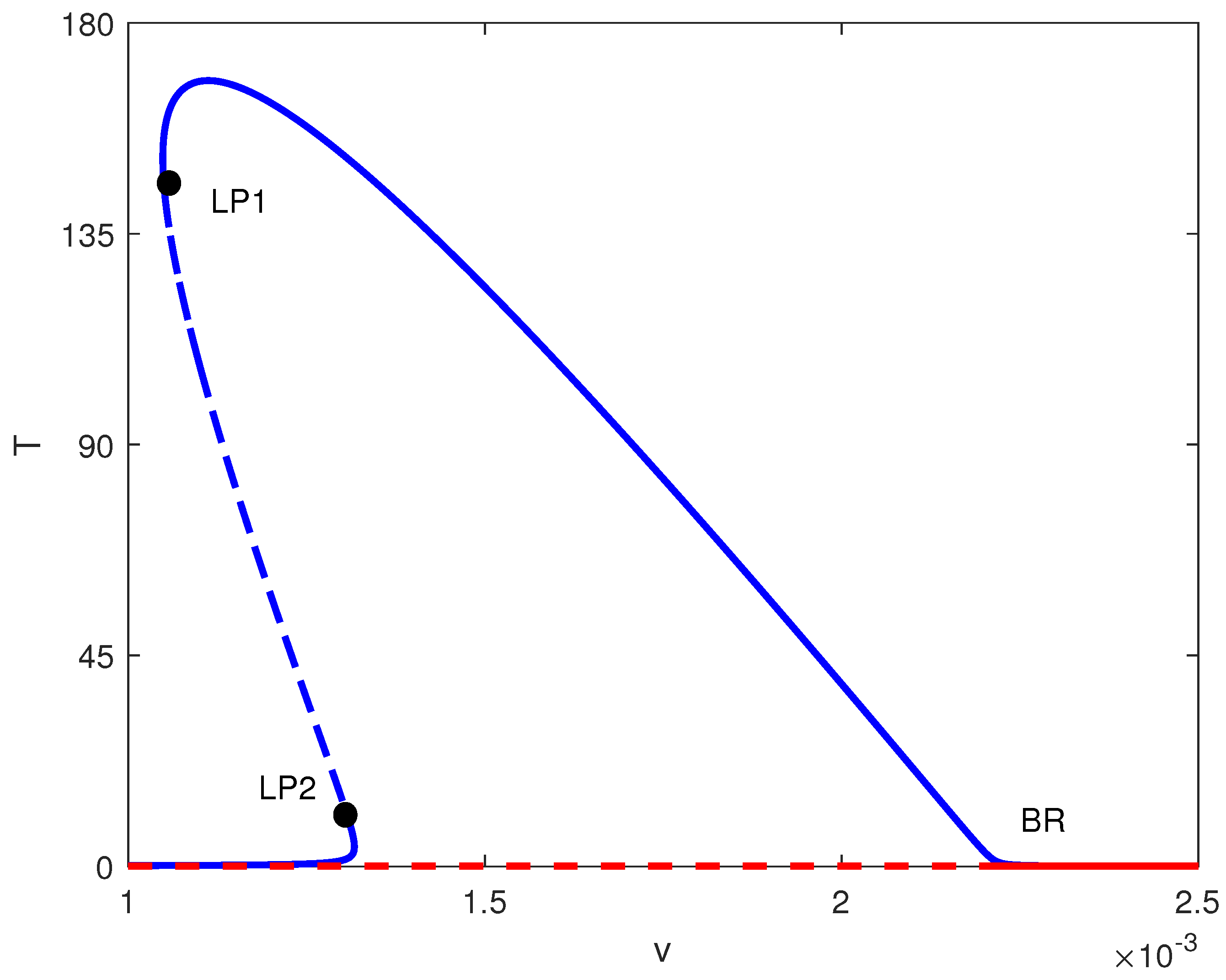
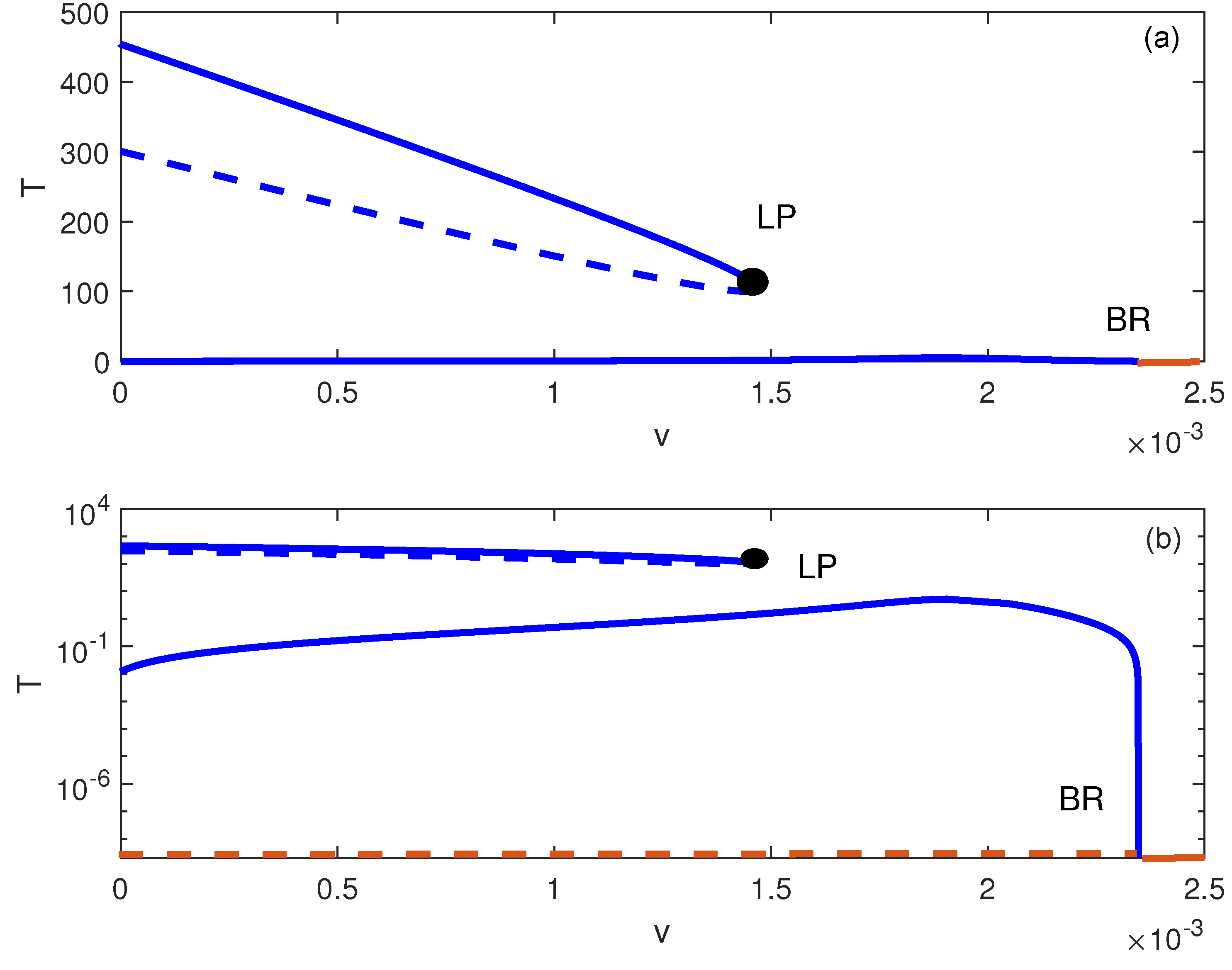
The branch sets for the different singularities are next constructed, for example, in the parameter space ( m , d ) . Figure 2 shows the hysteresis and isola/mushroom boundaries for the nominal values of the parameters in Equation (52). Region (1) has a unique solution. Figure 3 shows an example of a bifurcation diagram in this region in terms of drug intensity, for example, for ( m = 0.002 , d = 0.1 ) . It can be seen that for values of v larger than the bifurcation point B R , the trivial solution, i.e., T = 0 is the sole stable steady state. For v values below the B R , the system settles on a unique stable steady state. A feature of the model for this case is that as the drug intensity increases, the tumor continues to grow until it reaches a maximum value; beyond that, the tumor decreases until its eradication.
In region (2) of the branch set of Figure 2, two static limit points are born as a result of crossing the hysteresis line. An example of a bifurcation diagram is shown in Figure 4 for ( m = 0.002 , d = 0.4 ) . Two static limit points L P 1 and L P 2 occur at v = 0.001048 and v = 0.001316 , respectively. The following regimes are therefore expected: For v smaller than L P 1 , the system settles on the low-concentration tumor cells (the trivial solution T = 0 is unstable). Between L P 1 and L P 2 , there is bistability where the system can settle on low-tumor cells, but any changes in the initial conditions/external stimulations can push the system to sneak to a higher tumor concentration despite the administration of the drug. As the value of v increases beyond L P 2 , the tumor cell concentration decreases with the drug intensity. Values of v larger than the B R lead to suppression of the tumor.
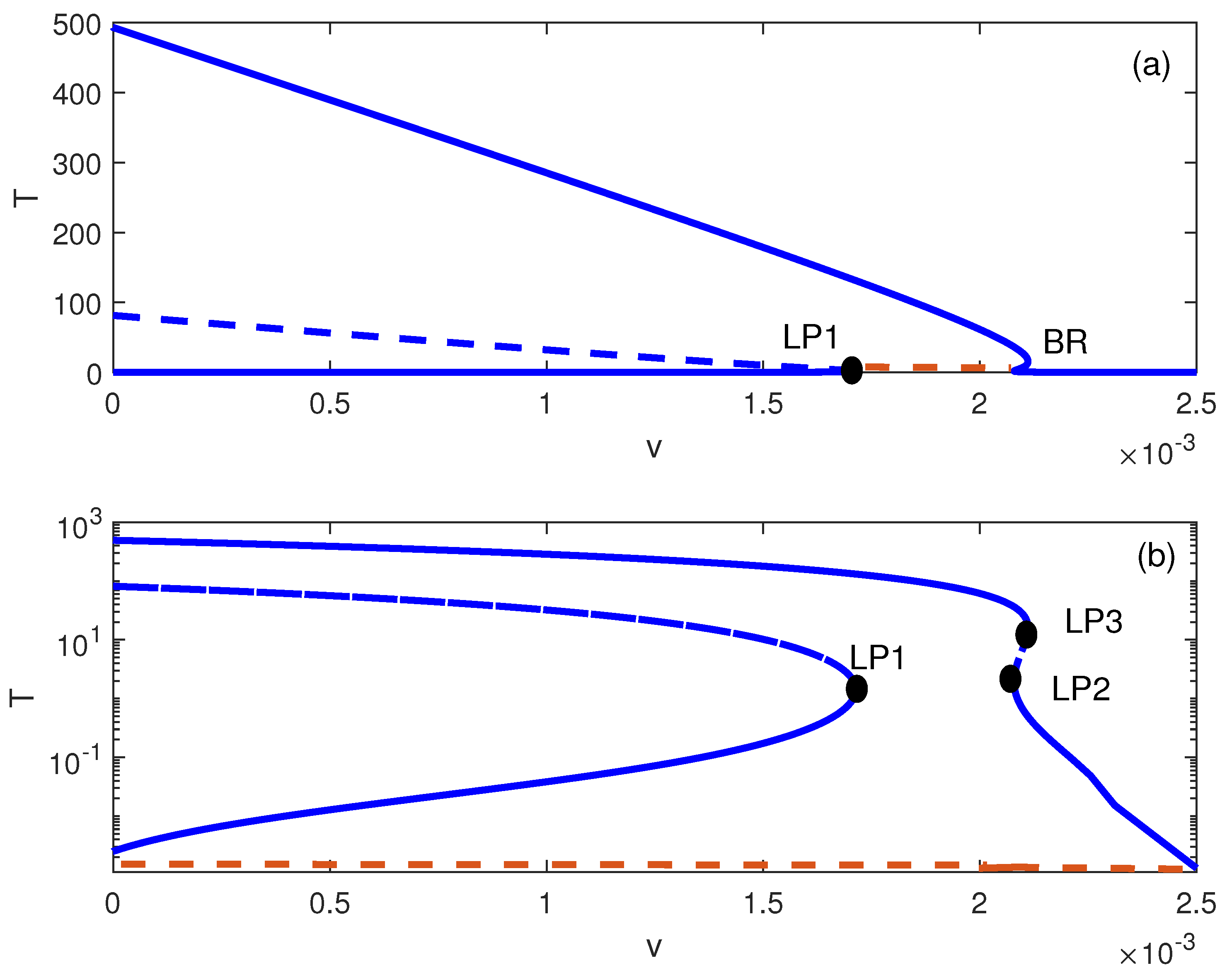
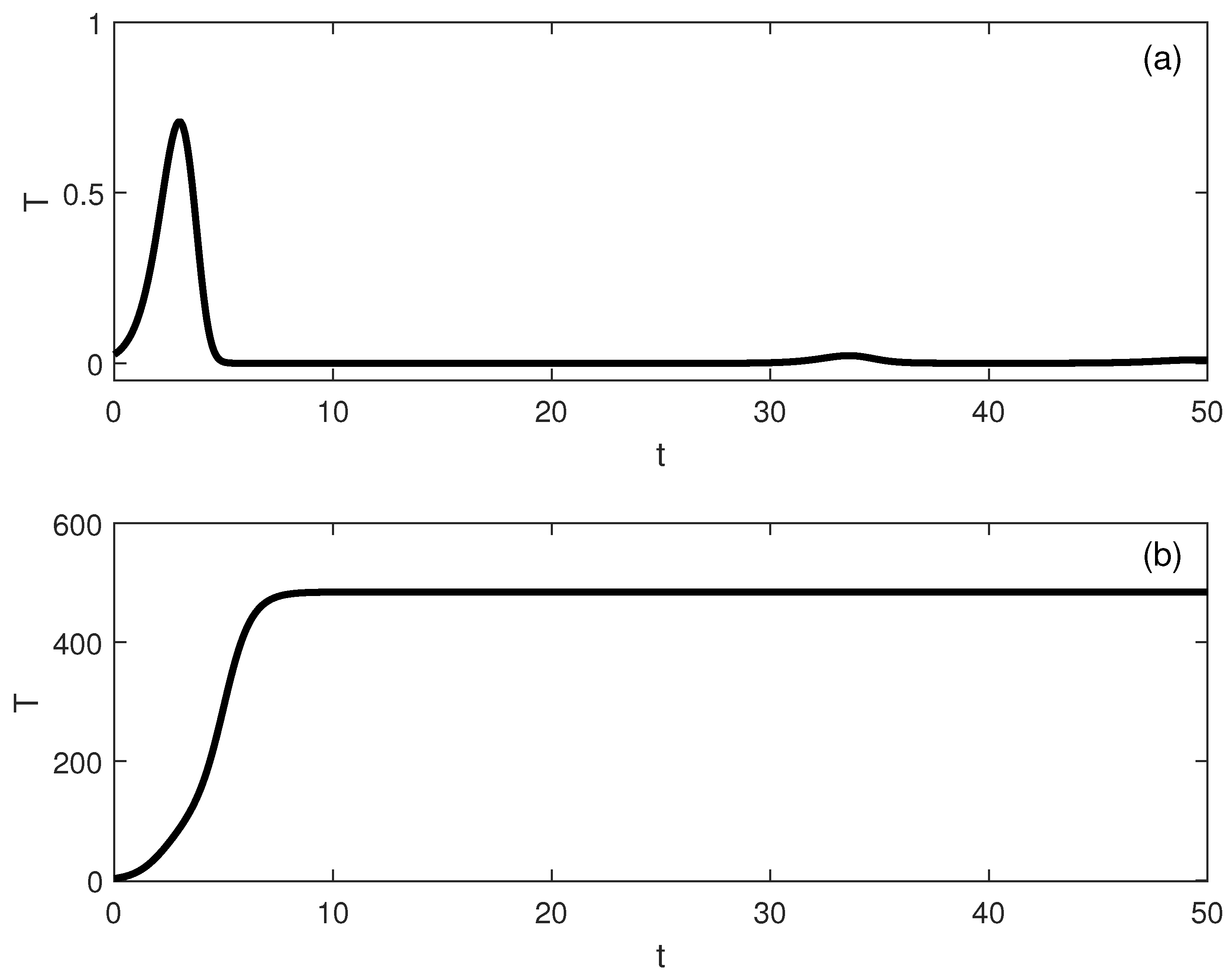
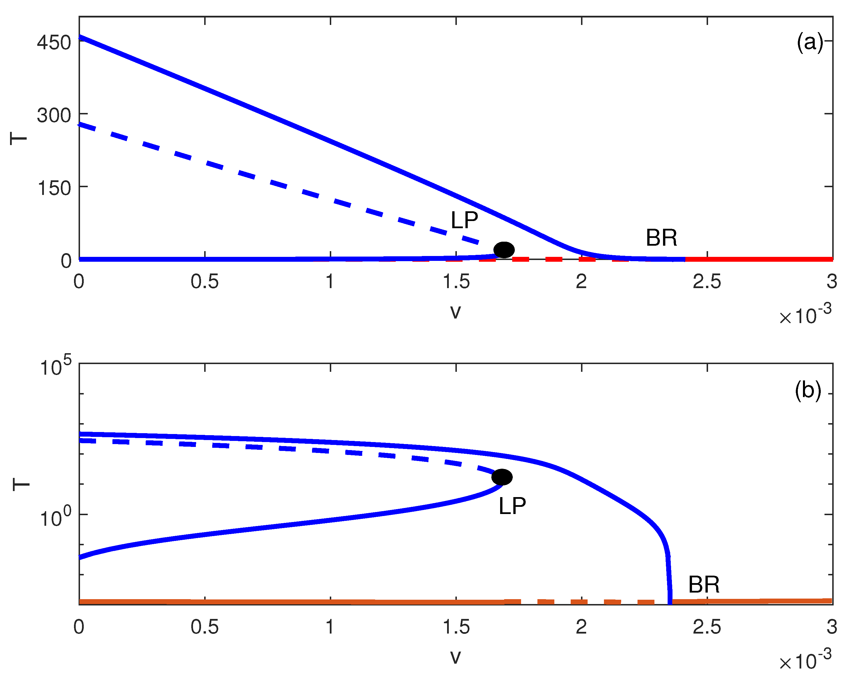
For region 3 of the branch set of Figure 2, an example of a bifurcation diagram is shown in Figure 5, for example, for ( m = 0.0125 , d = 0.2 ) . The diagram is more complex and shows the existence of a stable low-tumor concentration steady state (spiral), an unstable middle concentration steady state (saddle), and an upper stable steady state (node). Figure 5b shows a logarithmic plot (in y scale) for easier viewing. It can be seen that for v values smaller than L P 1 , ( v = 0.00171 ) , the low-cell branch coexists with the high-cell branch. Values of v larger than L P 1 and smaller than L P 2 , ( v = 0.00211 ) lead to high-tumor-cell concentration. In the small region between L P 2 , ( v = 0.00211 ) and L P 3 , ( v = 0.00218 ) , the high-tumor-cell branch coexists with the no-tumor steady state. As v values increase past L P 3 , the tumor cell concentration continues to decrease. Values of v larger than the B R lead to the suppression of the tumor. Time variations showing bistability are shown in Figure 6 for the value of v = 5 × 10 4 and two sets of initial conditions. Start-up conditions ( E , T , M ) = ( 1.3 × 10 2 , 2.6 × 10 2 , 6 × 10 5 ) lead after some transient oscillations (because of the spiral nature of the steady state) to the low-tumor steady state. On the other hand, the initial conditions ( E , T , M ) = ( 1.3 × 10 2 , 10 1 , 6 × 10 5 ) lead to the high-tumor steady state. Next, we examine the effect of the model parameters (other than m and d) on the hysteresis and isola/mushroom singularities. Figure 7 shows the results of the sensitivity analysis. In each case, a 25 percent change in the parameter is assumed. Figure 7a shows that an increase in the normal growth rate of effector cells from s = 0.12 to s = 0.15 increases the region of uniqueness as the regions of hysteresis and isola/mushroom move to higher values of d. Figure 7b shows that an increase in the value of p from 1.13 to 1.41 increases the region of uniqueness further compared to the effect of s. A decrease in the effect of k E from 5.45 to 4.08 (Figure 7c) has the effect of increasing the region of unique solution, while an increase in the value of k T from 5.45 to 6.81 (Figure 7d) has the same effect. Finally, the effect of g is the least pronounced, as shown in Figure 7e.
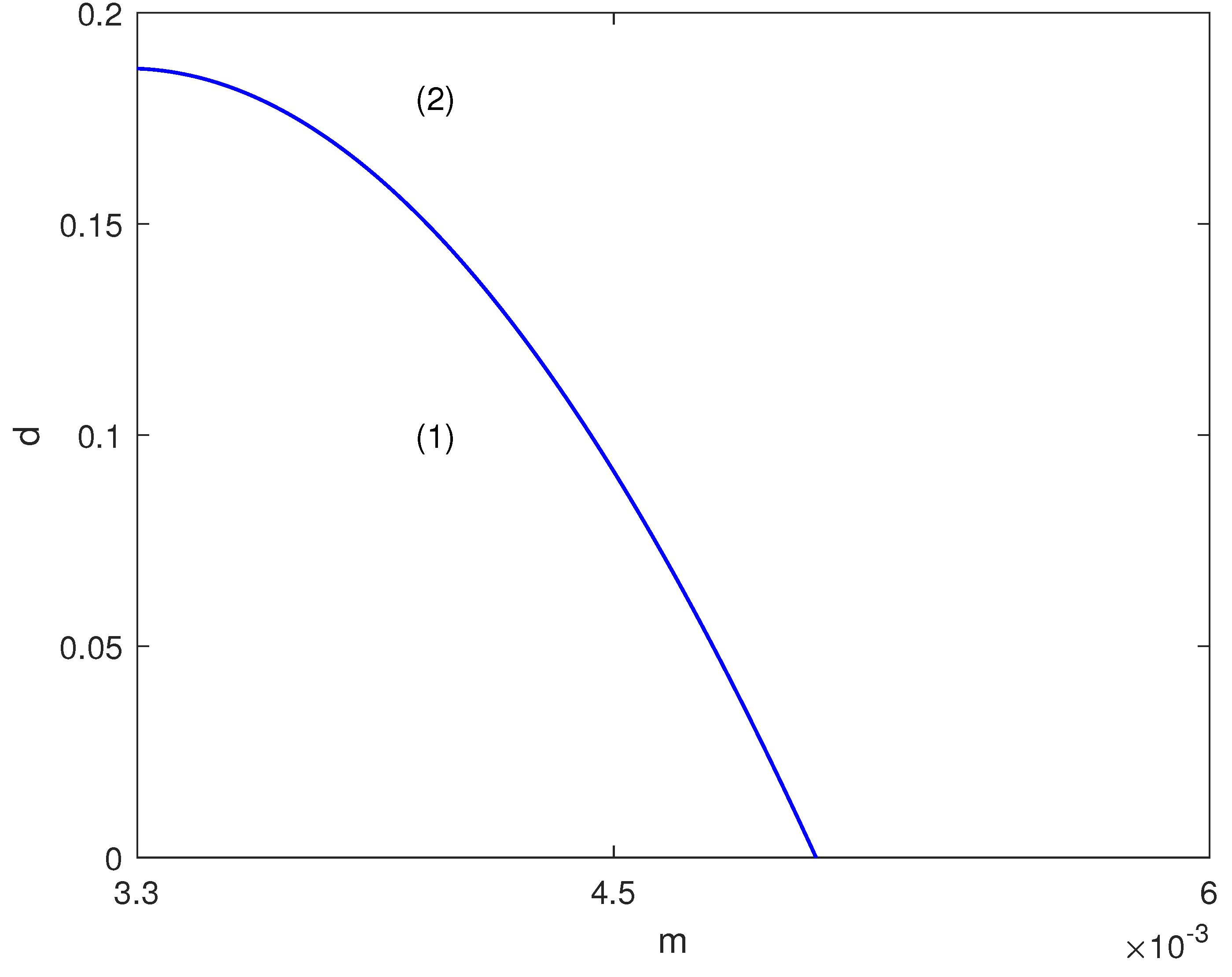
Next, we examine the occurrence of pitchfork singularity. Figure 8 shows the pitchfork boundary in the parameter space ( m , d ) . Figure 9 shows an example of a bifurcation diagram on the boundary itself of Figure 8, for example, for ( m = 0.004 , d = 0.1528 ) . A perfect pitchfork can be observed. (Figure 9b shows a logarithmic plot on the y axis of Figure 9a). For values of v up to the L P , there is coexistence between the low-tumor-cell and the high-tumor-cell branch. Beyond the L P and up to the B R , the tumor cell concentration decreases steadily as v increases. Beyond the value of the B R , the tumor is suppressed.
Figure 10 shows the behavior in region (1) of Figure 8, for example, for ( m = 0.004 ,   d = 0.11 ) . The perfect pitchfork of Figure 9 is perturbed, and the lower and upper stable branches are no longer connected. Values of v smaller than the L P lead to bistability, while values larger than the L P and up to the B R lead to low-concentration stable steady state. Values of v larger than the B R lead to suppression of the tumor.
Figure 11 shows an example of a bifurcation diagram in region (2) of Figure 8, for example, for ( m = 0.004 , d = 0.18 ) . The perfect pitchfork is again perturbed. However, from a practical point of view, the behavior of Figure 11 is similar to that of Figure 10. The only difference between Figure 10 and Figure 11 is the presence of a maximum in Figure 10, while the tumor cell concentration in Figure 11 decreases steadily after the L P .
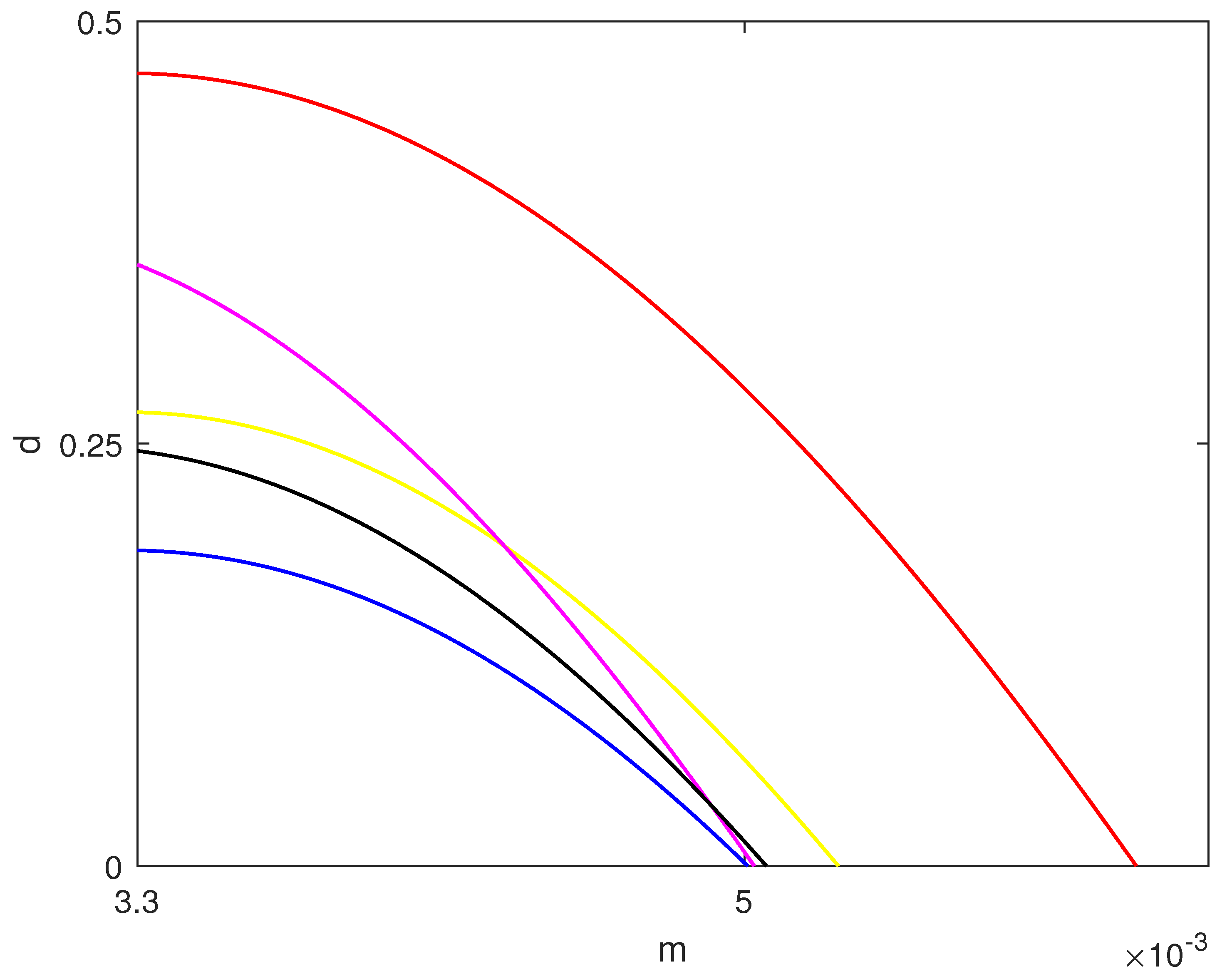
Figure 12 shows the effect of model parameters on the limits of pitchfork singularity. It can be seen that compared to the nominal case (blue line), an increase in the value of s by 25% (yellow line) increases the pitchfork boundary, as the boundary occurs at larger values of d. The effect of the increase in p by 25% (red line) is very pronounced. A decrease in the value of k E (magenta line) or an increase in k T (black line) increases the pitchfork boundary.
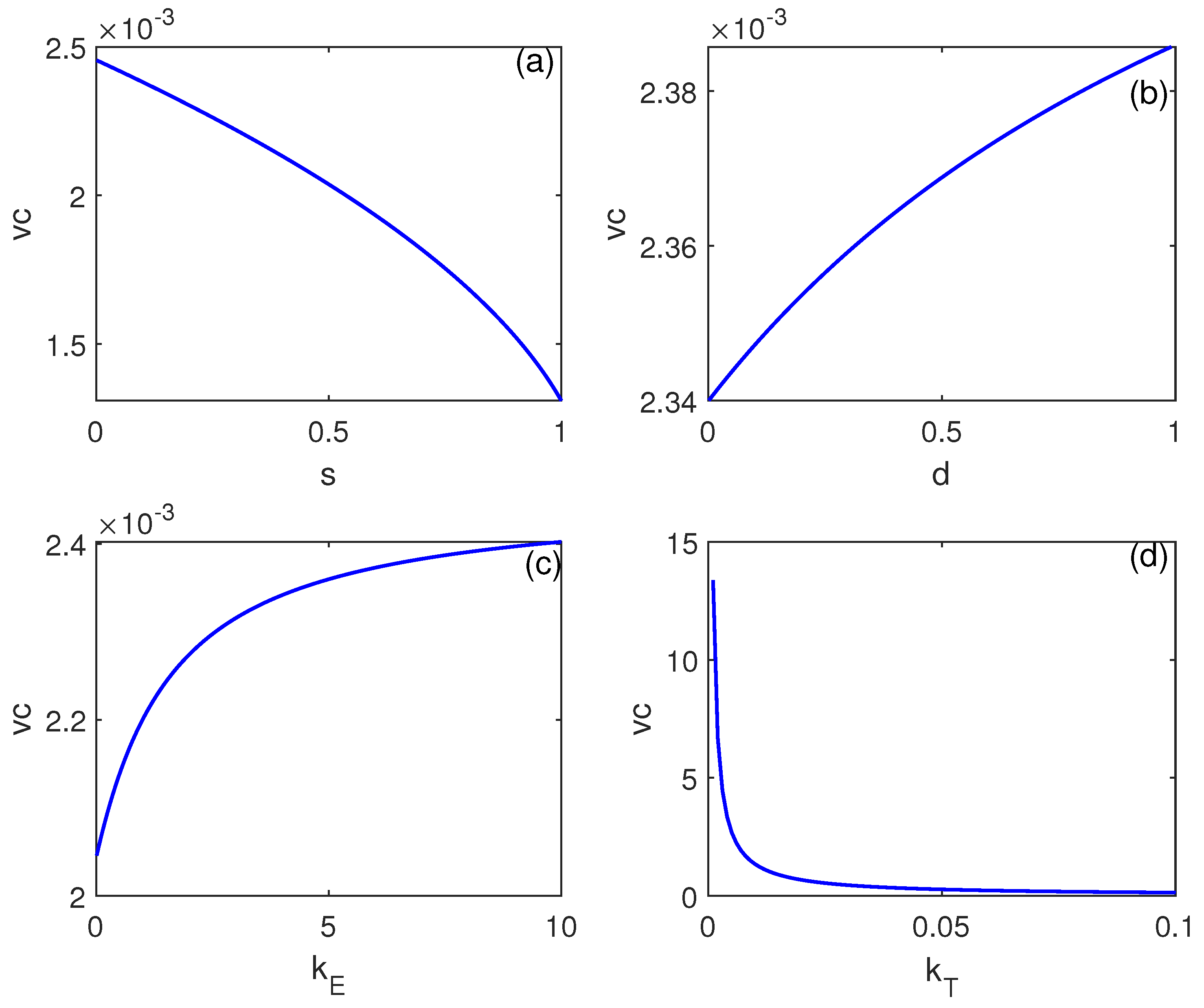
Finally, we saw in all the aforementioned bifurcation diagrams that if the drug intensity is increased past a critical point ( v c ) solution of a 0 = 0 (Equation (15)), the tumor is completely suppressed. Figure 13 shows the effect of the different model parameters on the critical value ( v c ) . It can be seen that as s is increased, v c decreases, while the opposite can be seen for d. As k E increases, v c increases, while k T has the opposite effect and is more pronounced. The value of v c is independent of β , g, p, and m.

6. Discussion

The theoretical analysis using the singularity theory has shown that small variations in the model’s biological parameter values can lead to a number of bifurcation patterns. In real life, it is feasible for biological parameter values to vary given that both effector and tumor cell populations are heterogeneous, comprising different subpopulations that possess distinct parameter values influencing their behavior.
The model without chemotherapy was studied in [9], and the authors showed the presence of hysteresis, which is marked by the coexistence of areas with low-tumor-cell concentrations alongside regions with high concentrations as well as regions where “dormant cells” can evade regulatory effects from effectors and subsequently become active. Saddle node and transcritical bifurcations were also shown to exist [25,26] in such models.
With the introduction of chemotherapy, the analysis has revealed that the model is capable of predicting a greater range of behaviors than what was identified in earlier studies [9,25,26].
For some values of model biological parameters, the effector system is efficient, and the model can only predict a low-tumor-cell steady state. However, when the level of administrated drug is increased, the tumor cell concentration does not, as expected, decrease monotonically. Rather, and as result of the complex interactions between the model’s biological parameters and those associated with the chemotherapy, the tumor cell concentration increases and reaches a maximum before decreasing. Only drug levels past a critical level (Equation (15)) can completely suppress the tumor. For this combination of biological and chemotherapy parameters, the administration of the drug at intermediate doses (relative to the critical value, Equation (15)) can be detrimental to the disease outcome.
For other values of model biological parameters, the model forecasts a hysteresis. It was observed that relatively low drug levels can stabilize the system at low-tumor-cell populations. However, increasing the drug level may push the system into the zone of hysteresis, where a sneaking phenomenon can push the tumor from low- to high-tumor-cell populationss as a result of changes in the initial conditions and/or external stimulations. Again, only large values of drug administration past a critical threshold can eradicate the tumor. For this scenario, it is advised to avoid administrating the drug at levels within the hysteresis region.
Pitchfork singularities, either perfect or in perturbed forms, were found to also occur in the model for some range of parameters. In these cases, the effector system is less efficient, and even for small doses of chemotherapy, the system exhibits bistability between the low-tumor and high- (uncontrolled) tumor-cell populations. If the drug levels are increased past the bistability domain of the pitchfork, then either the tumor cells decrease monotonically or unexpectedly increase, reaching a maximum before decreasing. For these sets of conditions, it is advised to increase the drug past low values of bisability but below the peak of tumor cell concentration.
Together with chemotherapy, immunotherapy may act as a treatment that influences systemic parameters, such as the sustained elevation of the cytolytic potential of immune killer cells, which is indicated by the parameter (n) in Equation (2). If the systems parameters can be altered, then in order to avoid bistability, the region of unique steady state was found to be favored by an increase in the growth rate of the effector cells, a decrease in their death rate, an increase in the degree of recruitment of maximum immune effector cells in relation to cancer cells, an increase in the effect of chemotherapy on tumor cells, and a decrease in the effect of chemotherapy on effector cells. The degree of recruitment of maximum immune effector cells in relation to cancer cells had, on the other hand, the least pronounced effect.
Additionally, in all the uncovered bifurcation patterns, the tumor can be completely eradicated if the chemotherapy is increased past a critical value. A simple analytical expression (Equation (15)) was found for this value. This critical value decreases when the effector cells’ normal growth rate is increased and/or death rate decreases or when the growth rate ( α ) of the tumor decreases. The critical value also depends on the chemotherapy drug parameters, where it can be decreased by an increase in the rate of response coefficient affecting the tumor cells or a decrease in the response coefficient affecting the effector cells.
In relation to the topic of oscillations, we have demonstrated that the proposed model does not have the capability to predict any oscillatory behavior, regardless of the model parameters. Population size fluctuations are an essential element of the interactions that occur between predators and prey. Established models of predator–prey interactions account for these oscillations by utilizing suitable functional responses or by introducing delays within the model, among other factors [19,23]. The lack of oscillatory behavior in the proposed competition model is worthy of discussion. It is probably advantageous for tumor cells to induce fluctuations in the human body, as this can enable a temporary avoidance of the immune system and lead to a higher rate of tumor spread. This has been demonstrated in certain diseases, such as malaria [33] and smallpox [34]. However, oscillations in the context of tumor–immune cell interactions have not yet been confirmed [19,35]. Several interpretations were suggested [19,21], but the most plausible explanation is the potential risk of autoimmune reactions, which may endanger the stability of healthy cells. Attaining a state of comprehensive homeostasis within the body amidst the complex interactions between tumor and immune cells poses significant challenges, as the dedication to generating immune cells can disrupt other physiological processes. For this reason, I maintain that a suitable model that effectively represents the dynamics of tumor–immune interactions should refrain from predicting periodic or aperiodic behavior, at least within the acceptable range of model parameters.
Additionally, since the nominal values of the model’s parameters were taken from realistic conditions [9,16], the objective of any future work is to validate the model by comparing all the uncovered bifurcation behavior to real-life outcomes. It should be noted that hysteresis, saddle node, and transcrtical bifurcation are known to occur experimentally [9,25,26]. The rest of the branching phenomena needs to be validated. But at this point, it is essential to highlight that the bifurcation phenomena observed in the model, as shown in the corresponding figures, occurred when the dimensionless drug intensity was less than approximately 3 × 10 3 . It is a well-established fact that the total amount of chemotherapy administered during treatment is limited, as it adversely affects both cancerous and normal cells. Guidelines indicate that chemotherapy doses can reach as high as 3500 mg/m2 per day [36]. Utilizing the dimensionless variables in Equation (5), this corresponds to a dimensionless drug intensity of about 3.2   ×   10 3 , which is greater than the maximum value used in this analysis. This observation confirms that the range selected for this study is realistic.
A final note should be made about the limitations of the current work. The chemotherapy effect on both effector and tumor cells was described by a simple mass action linear model through the parameters k E and k T (Equations (1) and (2)). Other expressions were also used in the literature such as a saturation type, e.g., k T ( 1 + h T ) [20], or the exponential kill model with a time-delayed concentration, e.g., k ( 1 e M ) [26]. The extension of the results of this paper to these models is worth investigating.

7. Conclusions

The purpose of this work was to analyze the different bifurcation solutions that can be displayed by a simple model describing effector–tumor cell interactions under chemotherapy. The mathematical analysis using singularity theory managed to delineate the complex interactions between the model’s biological and chemotherapy parameters that results in a number of bifurcation phenomena.
For particular values of the model’s biological parameters, there exists solely a stable equilibrium. The concentration of tumor cells escalates with increasing drug intensity, attains a peak, and then diminishes, culminating in their elimination at higher drug doses.
For other values of model biological parameters, a hysteresis occurs and implies that within specific ranges of drug dose, a sneaking phenomenon could lead to an increase in tumor cell numbers, driven by changes in the initial conditions and/or external influences.
In other cases, the system shows bistability at low doses of chemotherapy between a reduced number of tumor cells and those that are uncontrolled. If the dosage surpasses the bistability threshold, the tumor cells may either decrease in a consistent manner or, counterintuitively, increase to a peak before declining.
Finally, the relevance of these mathematical models is not confined to understanding how intrinsic parameters or chemotherapy affect the emergence of different bifurcations and bistability. After identifying these patterns, the next phase is to apply these models to explore various other issues, including the merit of periodic adjustment of drug doses and evaluating the optimal rate of drug administration during patient treatment by treating the medication as a control function v ( t ) . This is especially important for minimizing the risk of drug toxicity. Additionally, identifying the best timing for each drug injection represents another critical optimal control problem that requires further research.

Funding

This work was supported and funded by the Deanship of Scientific Research at Imam Mohammad Ibn Saud Islamic University (IMSIU) (grant number IMSIU-DDRSP2501).

Data Availability Statement

The original contributions presented in the study are included in the article; further inquiries can be directed to the corresponding author.

Conflicts of Interest

The authors declare no conflicts of interest.

References

  1. Bray, F.; Laversanne, M.; Sung, H.; Ferlay, J.; Siegel, R.L.; Soerjomataram, I.; Jemal, A. Global cancer statistics 2022: GLOBOCAN estimates of incidence and mortality worldwide for 36 cancers in 185 countries. CA Cancer J. Clin. 2024, 74, 229–263. [Google Scholar] [CrossRef] [PubMed]
  2. Rockne, R.C.; Scott, J.G. Introduction to Mathematical Oncology. JCO Clin. Cancer Inform. 2019, 3, 1–4. [Google Scholar]
  3. Araujo, R.P.; McElwain, D.L.S. A history of the study of solid tumour growth: The contribution of mathematical modelling. Bull. Math. Biol. 2004, 66, 1039–1091. [Google Scholar] [CrossRef] [PubMed]
  4. Enderling, H.; Wolkenhauer, O. Are all models wrong? Comput. Syst. Oncol. 2020, 1, e1008. [Google Scholar]
  5. Batmani, Y.; Khaloozadeh, H. Optimal drug regimens in cancer chemotherapy: A multi-objective approach. Comput. Biol. Med. 2013, 43, 2089–2095. [Google Scholar]
  6. Agur, Z.; Vuk-Pavlovic, S. Mathematical modeling in immunotherapy of cancer: Personalizing clinical trials. Mol. Ther. 2012, 20, 1–2. [Google Scholar]
  7. Wang, Z.; Deisboeck, T.S. Mathematical modeling in cancer drug discovery. Drug Discov. Today 2014, 19, 145–150. [Google Scholar]
  8. Yin, A.; Moes, D.J.; van Hasselt, J.G.; Swen, J.J.; Guchelaar, H.J. A review of mathematical models for tumor dynamics and treatment resistance evolution of solid tumors. CPT Pharmacometrics Syst. Pharmacol. 2019, 8, 720–737. [Google Scholar]
  9. Kuznetsov, V.A.; Makalkin, I.A.; Taylor, M.A.; Perelson, A.S. Nonlinear dynamics of immunogenic tumors: Parameter estimation and global bifurcation analysis. Bull. Math. Biol. 1994, 56, 295–321. [Google Scholar]
  10. Robertson-Tessi, M.; El-Kareh, A.; Goriely, A. A mathematical model of tumor-immune interactions. J. Theor. Biol. 2012, 294, 56–73. [Google Scholar] [CrossRef]
  11. Kaur, G.; Ahmad, N. On study of immune response to tumor cells in prey-predator system. Int. Sch. Res. Not. 2014, 2014, 346597. [Google Scholar] [CrossRef]
  12. Benzekry, S.; Lamont, C.; Beheshti, A.; Tracz, A.; Ebos, J.M.; Hlatky, L.; Hahnfeldt, P. Classical mathematical models for description and prediction of experimental tumor growth. PLoS Comput. Biol. 2014, 10, e1003800. [Google Scholar] [CrossRef] [PubMed]
  13. Michor, F.; Beal, K. Improving cancer treatment via mathematical modeling: Surmounting the challenges is worth the effort. Cell 2015, 163, 1059–1063. [Google Scholar] [CrossRef] [PubMed]
  14. Murphy, H.; Jaafari, H.; Dobrovolny, H.M. Differences in predictions of ODE models of tumor growth: A cautionary example. BMC Cancer 2016, 16, 163. [Google Scholar] [CrossRef]
  15. Heesterman, B.L.; Bokhorst, J.M.; de Pont, L.M.; Verbist, B.M.; Bayley, J.P.; van der Mey, A.G.; Corssmit, E.P.; Hes, F.J.; van Benthem, P.P.; Jansen, J.C. Mathematical models for tumor growth and the reduction of overtreatment. J. Neurol. Surg. B Skull Base 2019, 80, 72–78. [Google Scholar] [CrossRef]
  16. Lestari, D.; Sari, E.R.; Arifah, H. Dynamics of a mathematical model of cancer cells with Chemotherapy. J. Phys. Conf. Ser. 2019, 1320, 012026. [Google Scholar] [CrossRef]
  17. Akhmetzhanov, A.R.; Kim, J.W.; Sullivan, R.; Beckman, R.A.; Tamayo, P.; Yeang, C.H. Modelling bistable tumour population dynamics to design effective treatment strategies. J. Theor. Biol. 2019, 474, 88–102. [Google Scholar] [CrossRef]
  18. Beckman, R.A.; Kareva, I.; Adler, F.R. How should cancer models be constructed? Cancer Control 2020, 27, 1073274820962008. [Google Scholar] [CrossRef]
  19. Kareva, I.; Luddy, K.A.; O’Farrelly, C.; Gatenby, R.A.; Brown, J.S. Predator-prey in tumor-immune interactions: A wrong model or just an incomplete one? Front. Immunol. 2021, 12, 668221. [Google Scholar] [CrossRef]
  20. Bashkirtseva, I.; Chukhareva, A.; Ryashko, L. Modeling and analysis of nonlineartumor-immune interaction under chemotherapy and radiotherapy. Math. Methods Appl. Sci. 2022, 45, 7983–7991. [Google Scholar] [CrossRef]
  21. Hamilton, P.T.; Anholt, B.R.; Nelson, B.H. Tumour immunotherapy: Lessons from predator-prey theory. Nat. Rev. Immunol. 2022, 22, 765–775. [Google Scholar] [CrossRef] [PubMed]
  22. Kareva, I.; Berezovskaya, F. Cancer immunoediting: A process driven by metabolic competition as a predator-prey-shared resource type model. J. Theor. Biol. 2015, 380, 463–472. [Google Scholar] [PubMed]
  23. Bazykin, A.D. Nonlinear Dynamics of Interacting Populations; World Scientific: Singapore, 1998. [Google Scholar]
  24. Golubovskaya, V.; Wu, L. Different Subsets of T Cells, Memory, Effector Functions, and CAR-T Immunotherapy. Cancers 2016, 8, 36. [Google Scholar] [CrossRef] [PubMed]
  25. De Pillis, L.G.; Radunskaya, A.E. Modeling tumor-immune dynamics, In Mathematical Models of Tumor-Immune System Dynamics; Eladdadi, A., Kim, P., Mallet, D., Eds.; Springer Proceedings in Mathematics & Statistics 107; Springer Science+Business Media: New York, NY, USA, 2014; pp. 59–108. [Google Scholar]
  26. López, A.G.; Seoane, J.M.; Sanjuán, M.A. A validated mathematical model of tumor growth including tumor-host interaction, cell-mediated immune response and chemotherapy. Bull. Math. Biol. 2014, 76, 2884–2906. [Google Scholar]
  27. Makhlouf, A.M.; El-Shennawy, L.; Elkaranshawy, H.A. Mathematical modelling for the role of CD4+T cells in tumor-immune interactions. Comput. Math. Methods Med. 2020, 2020, 7187602. [Google Scholar] [CrossRef]
  28. Song, G.; Tian, T.; Zhang, X. A mathematical model of cell-mediated immune response to tumor. Math. Biosci. Eng. 2020, 18, 373. [Google Scholar]
  29. Wiggins, S. Introduction to Applied Nonlinear Dynamical Systems and Chaos; Springer: New York, NY, USA, 1990. [Google Scholar]
  30. Golubitsky, M.; Stewart, I.; Schaeffer, D.G. Singularities and Groups in Bifurcation Theory: Volume II; Springer: Berlin/Heidelberg, Germany, 1988. [Google Scholar]
  31. Alhumaizi, K.; Aris, R. Surveying a Dynamical System: A Study of the Gray-Scott Reaction in a Two-Phase Reactor; Research Notes in Mathematics Series; Chapman & Hall/CRC: London, UK, 1995. [Google Scholar]
  32. Ajbar, A.; Alhumaizi, K. Dynamics of the Chemostat: A Bifurcation Theory Approach; Chapman and Hall/CRC: London, UK, 2011. [Google Scholar]
  33. Smith, L.M.; Motta, F.C.; Chopra, G.; Moch, J.K.; Nerem, R.R.; Cummins, B.; Roche, K.E.; Kelliher, C.M.; Leman, A.R.; Harer, J.; et al. An intrinsic oscillator drives the blood stage cycle of the malaria parasite Plasmodium falciparum. Science 2020, 368, 754. [Google Scholar]
  34. Greer, M.; Saha, R.; Gogliettino, A.; Yu, C.; Zollo-Venecek, K. Emergence of oscillations in a simple epidemic model with demographic data. R. Soc. Open Sci. 2020, 7, 191187. [Google Scholar]
  35. Dorraki, M.; Fouladzadeh, A.; Salamon, S.J.; Allison, A.; Coventry, B.J.; Abbott, D. On detection of periodicity in C-reactive protein (CRP) levels. Sci. Rep. 2018, 8, 11979. [Google Scholar] [CrossRef]
  36. Mazard, T.; Ychou, M.; Thezenas, S.; Poujol, S.; Pinguet, F.; Thirion, A.; Bleuse, J.P.; Portales, F.; Samalin, E.; Assenat, E. Feasibility of biweekly combination chemotherapy with capecitabine, irinotecan, and oxaliplatin in patients with metastatic solid tumors: Results of a two-step phase I trial: XELIRI and XELIRINOX. Cancer Chemother. Pharmacol. 2012, 69, 807–814. [Google Scholar]
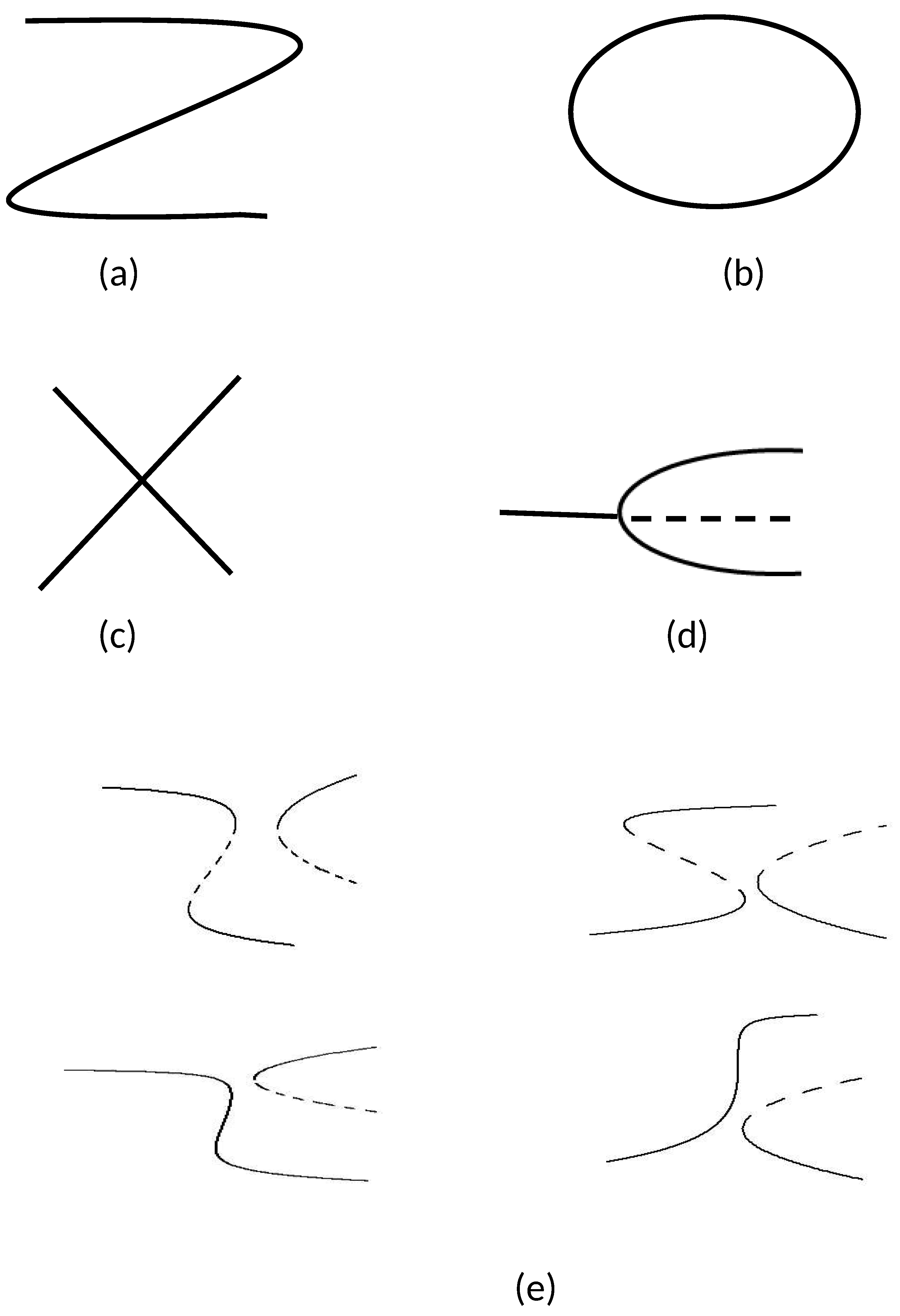
Figure 1. Basic singularities: (a) hysteresis; (b) isoal; (c) mushroom; (d) perfect pitchfork; (e) perturbed bifurcation diagrams for the pitchfork.
Mathematics 13 01032 g001
Figure 2. Hysteresis singularity (solid) and isola/mushroom singularity (dashed line) for model nominal values shown in Equation (52).
Mathematics 13 01032 g002
Figure 3. Bifurcation diagram for region (1) of Figure 2 for ( m = 0.002 , d = 0.1 ) ; solid line (stable branch); dashed line (unstable branch); BR (bifurcation point). Blue color nontrivial steady-state; Red color trivial steady-state ( T = 0 ) .
Mathematics 13 01032 g003
Figure 4. Bifurcation diagram for region (2) of Figure 2 for ( m = 0.002 , d = 0.4 ) : solid line (stable branch); dashed line (unstable branch); BR (bifurcation point). LP1 and LP2 limit points. Blue color is nontrivial steady state. Red color is trivial steady state ( T = 0 ) .
Mathematics 13 01032 g004
Figure 5. Bifurcation diagram for region (3) of Figure 2 for ( m = 0.0125 , d = 0.2 ) : (a) diagram in linear scale; (b) diagram in semi-logarithmic scale (in T); solid line (stable branch); dashed line (unstable branch); BR (bifurcation point); LP1, LP2, and LP3 limit points; blue color is nontrivial steady state; red color is trivial steady state ( T = 0 ) .
Mathematics 13 01032 g005
Figure 6. Simulations illustrating bistability in Figure 5, for example, for v = 5 × 10 4 . (a) Initial conditions ( E , T , M ) = ( 1.3 × 10 2 , 2.6 × 10 2 , 6 × 10 5 ) lead to low-tumor steady state. (b) Initial conditions ( E , T , M ) = ( 1.3 × 10 2 , 3 , 6 × 10 5 ) lead to the high-tumor steady state.
Mathematics 13 01032 g006
Figure 7. Effect of the different model parameters on the hysteresis and isola/mushroom singularities of Figure 2: (a) solid line ( s = 0.12 ), dashed line (s = 0.15). (b) solid line (p = 1.13), dashed line (p = 1.41). (c) solid line ( k E = 5.45 ), dashed line ( k E = 4.087 ). (d) solid line ( k T = 5.45 ), dashed line ( k T = 6.81 ). (e) solid line ( g = 0.02 ), dashed line ( g = 0.015 ).
Mathematics 13 01032 g007
Figure 8. Pitchfork singularity for nominal values shown in Equation (52).
Mathematics 13 01032 g008
Figure 9. (a) Bifurcation diagram showing a perfect pitchfork for the model parameters ( m = 0.004 , d = 0.1528 ) in the boundary between region (1) and (2) of Figure 8. (b) Diagram in semi-logarithmic scale (in T). Solid line (stable branch); dashed line (unstable branch); BR (bifurcation point); LP1 (limit point); blue color is nontrivial steady state; Red color is trivial steady state ( T = 0 ) .
Mathematics 13 01032 g009
Figure 10. (a) Bifurcation diagram for the model parameters ( m = 0.004 , d = 0.11 ) in region (1) of Figure 8. (b) Diagram in semi-logarithmic scale (in T). Solid line (stable branch); dashed line (unstable branch); BR (bifurcation point); LP (limit point); blue color is nontrivial steady state; red color is trivial steady state ( T = 0 ) .
Mathematics 13 01032 g010
Figure 11. (a) Bifurcation diagram for the model parameters ( m = 0.004 , d = 0.18 ) in region (2) of Figure 8. (b) Diagram in semi-logarithmic scale (in T). Solid line (stable branch); dashed line (unstable branch); BR (bifurcation point); LP (limit point); blue color is nontrivial steady state; red color is trivial steady state ( T = 0 ) .
Mathematics 13 01032 g011
Figure 12. Effect of the different model parameters on the pitchfork singularity of Figure 8. Blue line nominal case ( s = 0.12 , p = 1.13 , k E = 5.45 , k T = 5.45 ) ; yellow line (s = 0.15); red line (p = 1.41); magenta line ( k E = 4.63); black line ( k T = 5.72).
Mathematics 13 01032 g012
Figure 13. Effect model parameters on the critical value of drug intensity, past of which the tumor is suppressed. (a) Effect of s. (b) Effect of d. (c) Effect of k E . (d) Effect of k T .
Mathematics 13 01032 g013
Table 1. Number of positive roots of Equations (11)–(15).
Case a 3 a 2 a 1 a 0 Number of Sign ChangesNumber of Positive Roots
1++++00
2+++11
3+++22, 0
4++11
5+++22, 0
6++33, 1
7++22, 0
8+11
Disclaimer/Publisher’s Note: The statements, opinions and data contained in all publications are solely those of the individual author(s) and contributor(s) and not of MDPI and/or the editor(s). MDPI and/or the editor(s) disclaim responsibility for any injury to people or property resulting from any ideas, methods, instructions or products referred to in the content.