Article

Research on Internal Response in Three-Dimensional Elastodynamic Time Domain Boundary Element Method

1
College of Urban and Rural Construction, Hebei Agricultural University, Baoding 071001, China
2
Hebei Key Laboratory of Structural Safety and Low-Carbon Construction for Rural Buildings, Hebei Agricultural University, Baoding 071001, China
3
College of Civil Engineering and Architecture, Henan University of Technology, Zhengzhou 450001, China
4
School of Civil and Environmental Engineering, Harbin Institute of Technology (Shenzhen), Shenzhen 518055, China
*
Author to whom correspondence should be addressed.
Mathematics 2025, 13(7), 1025; https://doi.org/10.3390/math13071025
Submission received: 25 February 2025 / Revised: 14 March 2025 / Accepted: 19 March 2025 / Published: 21 March 2025

Abstract

:
This study extends the calculation of unknown quantities at boundary points to the computation of internal displacements and stresses. The methodological approach is broadly consistent with boundary point calculations. However, the computation of internal unknowns does not involve spatial singularities; the internal stress boundary integral equation is first derived. Subsequently, the obtained boundary integral equation is numerically processed, requiring discretization in both time and space, followed by assembly and solution. When solving the elements in the influence coefficient matrices, the displacement influence coefficient matrix S and the traction influence coefficient matrix D exhibit only wavefront singularities. These wavefront singularities are treated analytically in the time domain, and the spatial integrals are handled using Gaussian numerical integration. The correctness of the algorithm and theory is verified through two classical numerical examples. A theoretically sound and accurate three-dimensional elastodynamic time domain boundary element method and its corresponding computational program are established, providing a reliable tool for guiding engineering design.

1. Introduction

With the continuous development of computer science and technology, the advancement of numerical methods has been rapid, making them an essential tool for solving practical engineering and scientific and societal problems. The boundary element method (BEM) offers significant advantages over other numerical methods, as it requires discretization only along the boundaries of the problem domain. The time domain boundary element method (TD-BEM) directly performs calculations in the time domain without any transformations, providing strong adaptability and stability. As a result, it has been widely applied to problems involving semi-infinite or infinite domains [1,2,3]. The BEM typically studies unknown quantities at boundary points. However, practical engineering problems often require understanding the domain’s internal responses, such as the tension and shear in beams or the compression and tension in columns. Therefore, research on internal responses holds significant engineering relevance.
Scholars’ exploration of the BEM domestically and internationally began in the 1950s and 1960s, and the formation and refinement of its theoretical framework underwent a prolonged process. The introduction of Green’s functions laid down the theoretical foundation for the BEM [4]. Subsequently, in the 1950s, Kupradze and Jaswon further developed the concept of boundary integral equations [5,6]. In 1977, Brebbia, Dominguez, Banerjee, and Butterfield formally named this approach the “boundary element method” and published the first monograph on the subject, titled The Boundary Element Method for Engineers [7]. This landmark work holds profound significance for the development of BEM. In the early stages of developing the TD-BEM, Mansur and Brebbia, in their work [8], presented integral equations for two-dimensional and three-dimensional transient problems governed by the scalar wave equation. This contribution laid a solid foundation for establishing the complete time domain boundary integral equations. Subsequently, Karabalis and Beskos [1] proposed transient time domain boundary integral equations for three-dimensional elastodynamics in soil–structure interaction problems. Banerjee [9] studied three-dimensional TD-BEM and proposed numerical methods for treating wavefront singularities and weak spatial singularities. Additionally, hyper singularities were addressed using the rigid body displacement method. Due to its simplicity in principle and ease of numerical implementation, the rigid body displacement method quickly gained widespread adoption [10,11]. In 1995, Coda et al. [12] investigated the interaction between building structures and foundations, researching the three-dimensional TD-BEM. They proposed numerical methods for handling temporal singular integrals over planar triangular and quadrilateral elements while employing Kutt’s quadrature method to compute spatial singular integrals. Kutt’s quadrature effectively resolves spatial singularity issues by performing a weighted summation of the integrand at selected nodes while retaining the finite part of the integral. This method has since been widely adopted by researchers [13,14]. In 2011, Panagiotopoulos and Manolis [15] established time domain boundary integral equations for three-dimensional elastodynamics based on the velocity reciprocity theorem. They linked the velocities and tractions of two different elastodynamic states of the same object, requiring only the substitution of the displacement fundamental solution with the corresponding velocity solution. This formulation reduced numerical instability and eliminated issues of “intermittency” and “burstiness”. When studying three-dimensional elastic problems using TD-BEM, Qin et al. discovered that spatial singularities cannot exist independently; only wavefront and double singularities are present. Based on the propagation characteristics of P-waves and S-waves, as well as the properties of the Heaviside function, Dirac function, and its derivatives, they identified the Analytically Time-Integrable Temporal–Spatial Domain (ATI-TSD) for double singular integrals. They then directly addressed spatial singularities using Kutt’s quadrature formula [16,17]. In summary, the development of the three-dimensional elastodynamic TD-BEM has undergone a lengthy process, evolving from establishing theoretical frameworks to optimizing numerical methods [18,19,20] and expanding its application scope.
In studying the three-dimensional elastodynamic TD-BEM, the computation of internal responses is also a significant research direction. Israil and Banerjee [21] proposed an improved time domain boundary element formulation for determining internal stresses. They derived a new set of more straightforward and efficient transient dynamic stress kernels, transforming the non-integrable wavefront singularities in the integral stress kernels into integrable singularities. The accuracy and stability of this method were validated through several numerical examples, including cases considering the stress concentration. Carrer and Mansur [22] computed stress and velocity components in two-dimensional elastodynamic problems. By differentiating the displacement fundamental solution concerning time, they obtained the velocity fundamental solution and established the velocity integral equation. They employed Hadamard finite part integrals to resolve wavefront singularities analytically. In contrast, spatial and double singularities were numerically treated using the rigid body displacement method, achieving satisfactory results for both velocities and stresses. To improve the accuracy of internal stress computations, Beskos proposed enhanced numerical integration techniques [2]. Schanz and Antes [23] conducted internal stress calculations for viscoelastic materials, yielding promising results. Additionally, several scholars have made significant progress in the study of internal stresses [24,25]. However, domestic and international scholars’ research on internal stresses in three-dimensional elastodynamics remains relatively limited. Therefore, this paper focuses on the study of internal stresses in three-dimensional elastodynamic TD-BEM.
This study builds upon the existing research on the three-dimensional elastodynamic TD-BEM. It focuses on calculating internal responses, specifically internal displacements, stresses, and velocities. The fundamental approach is as follows: First, the internal displacement boundary integral equation is derived based on Graffi’s reciprocal theorem, followed by the stress boundary integral equation formulation. Subsequently, numerical treatment is applied to the integral equations, including discretization in time and space, the computation of element influence coefficients, and assembly and solution of the coefficient matrices. The velocity is computed using the finite difference method, where the internal displacements obtained from the calculations are converted into internal velocities through difference formulas. Notably, the wavefront singularities arising in the element influence coefficients are analytically treated, effectively eliminating the singularities. Finally, two numerical examples are provided to validate the accuracy of the internal point response calculated by TD-BEM.

2. Internal Point Boundary Integral Equation

Before calculating the internal response, obtaining the unknowns at all boundary points (including the boundary surface traction and displacements) is necessary. The displacements and surface traction can be determined by solving the displacement boundary integral equation of the TD-BEM for three-dimensional elastodynamics, as detailed in [16]. Once all unknown quantities at the boundary points have been solved, they can be substituted into the internal displacement integral equation to obtain the internal displacements.
Under the conditions of zero initial state and absence of body forces, the internal displacement boundary integral equation can be derived by applying Graffi’s dynamic reciprocal theorem. Point P is an internal point that does not coincide with point Q.
u i ( P , t ) = 0 t S u i k ( Q , P ; t τ ) p k ( Q , τ ) d S ( Q ) d τ 0 t S p i k ( Q , P ; t τ ) u k ( Q , τ ) d S ( Q ) d τ
where p i k and u i k denote the three-dimensional time domain fundamental solutions for traction and displacement, respectively. The fundamental solution was initially proposed by Stokes [26], Love [27], and De Hoop [28], and its form has continuously improved over time [29,30]. The version of the fundamental solution adopted in this study is derived from the work of Aliabadi [30]. Specifically, p i k represents the traction component in the xk-direction at the field point Q at time t, induced by a unit impulse force applied in the xi-direction at the source point P at time τ. Similarly, u i k represents the corresponding displacement component in the xk -direction.
u i k = 1 4 π μ ( ψ δ i k χ r , i r , k )
p i k = 1 4 π ψ r χ r ( r n δ i k + r , k n i ) 2 χ r ( r , i n k 2 r , i r , k r n ) 2 χ r r , i r , k r n + c 1 2 c 2 2 2 ψ r χ r 2 χ r r , i n k
The stress boundary integral equation can be derived based on the boundary integral, geometric, and constitutive equations.
σ i j ( P , t ) = S 0 t s i j k ( P , τ , Q , t ) u k ( Q , τ ) d τ d S + S 0 t d i j k ( P , τ ; Q , t ) p k ( Q , τ ) d τ d S
where Q and P denote the field and source points, respectively, and σ i j represents the stress at the source point. The terms d i j k and s i j k are the influence coefficient kernel functions derived from the traction fundamental solution and the displacement fundamental solution. In the derivation of Equations (5) and (6), both the derivatives of the source point displacement and traction concerning the source point coordinates are involved. The specific expressions are as follows:
d i j k = λ δ i j u m k , m + μ ( u i k , j + u j k , i ) = 1 4 π χ r ψ r δ i k r , j + δ k j r , i 2 χ r ( 2 r , i r , j r , k δ i j r , k ) + 2 χ r r , i r , j r , k + c 1 2 c 2 2 2 χ r + 2 χ r ψ r r , k δ i j
s i j k = λ δ i j p m k , m + μ ( p i k , j + p j k , i ) = μ 4 π 4 ( χ , r r 5 χ , r r + 8 χ r 2 ) A 1 ( ψ , r r ψ , r r 3 χ , r r + 6 χ r 2 ) A 01 + 2 γ A 02 2 ( ψ , r r χ r 2 ) B 1 + C 1 B 01
The coefficients in Equations (2), (3), (5) and (6) are as follows:
ψ = c 2 2 r 3 t   H t r c 2 H t r c 1 + 1 r δ t r c 2 χ = 3 ψ 2 r δ t r c 2 c 2 2 c 1 2 1 r δ t r c 1
ψ , r = ψ r = χ r 1 r 2 δ t r c 2 + r c 2 δ · t r c 2 χ , r = χ r = 3 χ r 1 r 2 δ t r c 2 + r c 2 δ · t r c 2 + c 2 2 c 1 2 1 r 2 δ t r c 1 + r c 1 δ · t r c 1
ψ , r r = 2 ψ r 2 = 4 χ r 2 + 1 r 3 3 δ t r c 2 + 3 r c 2 δ · t r c 2 + r 2 c 2 2 δ · · t r c 2 c 2 2 c 1 2 1 r 3 δ t r c 1 + r c 1 δ · t r c 1 χ , r r = 2 χ r 2 = 12 χ r 2 + 1 r 3 3 δ t r c 2 + 3 r c 2 δ · t r c 2 + r 2 c 2 2 δ · · t r c 2 c 2 2 c 1 2 1 r 3 5 δ t r c 1 + 5 r c 1 δ · t r c 1 + r 2 c 1 2 δ · · t r c 1
A 1 = r n r , k r , i r , j A 01 = r n ( δ i k r , j + δ j k r , i ) + r , k ( n j r , i + r , j n i ) A 02 = r n δ i j r , k + r , i r , j n k B 1 = δ j k n i + δ i k n j B 01 = δ i j n k γ = 2 χ , r r 4 χ r 2 + λ μ ( χ , r r + χ , r r 4 χ r 2 ψ , r r + ψ , r r ) C 1 = 4 χ r 2 + 4 λ μ ( χ , r r + 2 χ r 2 ψ , r r ) + λ 2 μ 2 ( χ , r r + 4 χ , r r + 2 χ r 2 ψ , r r 2 ψ , r r )
r i = r i Q r i P r , i = r x i Q = r x i P = r i r n i = x i n r n = r i n i
Equations (7)–(9) contain functions that induce wavefront singularities, where t = t τ , where the variable r denotes the distance from the source point to the field point, and H ( t r / c w ) , δ ( t r / c w ) , δ ˙ ( t r / c w ) , and δ ¨ ( t r / c w ) ( w = 1 ,   2 ) represent the Heaviside function, Dirac function, and the first- and second-order derivatives of the Dirac function, respectively. Equation (10) represents the expression for the kernel function, which is dependent on both time and space. The constants c 1 and c 2 represent the velocities of P-waves and S-waves, respectively. These are expressed by Equation (12), in which λ and μ denote the Lamé constants, ρ is the material density, and E and ν are Young’s modulus and Poisson’s ratio, respectively.
c 1 = λ ρ c 1 = λ + 2 μ ρ μ = E 2 ( 1 + ν ) λ = ν E ( 1 + ν ) ( 1 2 ν )

3. Numerical Processing

3.1. Numerical Discretization

The internal displacement and stress boundary integral equation is discretized in the time and space domains. In the time domain, a uniform time step discretization is applied, and linear interpolation functions are employed to ensure that both displacements and tractions vary linearly within each time step. In the spatial domain, quadrilateral elements discretize the displacements and tractions. After discretization in time and space, the displacement and stress boundary integral equation take the following form:
S 0 t u i k * p k ( Q , τ ) d τ d S ( Q ) = m = 0 M e = 1 N e a = 1 N q g i k m ; e , a p k m ; e , a S 0 t p i k * u k ( Q , τ ) d τ d S ( Q ) = m = 0 M e = 1 N e a = 1 N q h i k m ; e , a u k m ; e , a
S 0 t s i j k * p k ( Q , τ ) d τ d S ( Q ) = m = 0 M e = 1 N e a = 1 N q d i j k m ; e , a p k m ; e , a S 0 t d i j k * u k ( Q , τ ) d τ d S ( Q ) = m = 0 M e = 1 N e a = 1 N q s i j k m ; e , a u k m ; e , a
The terms g i k m ; e , a and h i k m ; e , a represent the influence coefficients of the field point tractions and displacements on the source point displacements, respectively, while the terms d i j k m ; e , a and s i j k m ; e , a denote the influence coefficients of the field point tractions and displacements on the source point stresses, for which the expressions are as Equations (15) and (16). u k m ; e , a denotes the displacement in the k-direction at the a-th node of element e at instant tm; p k m ; e , a represents the surface traction in the k-direction at the a-th node of element e at instant tm; N e , N q , and M are the total number of boundary elements, the total number of nodes in element e, and the total number of time steps, respectively.
g i k m , 2 ; e , a = S t m 1 t m u i k s τ t m 1 Δ t M a d τ d S g i k m + 1 , 1 ; e , a = S t m t m + 1 u i k s t m + 1 τ Δ t M a d τ d S h i k m , 2 ; e , a = S t m 1 t m p i k s τ t m 1 Δ t M a d τ d S h i k m + 1 , 1 ; e , a = S t m t m + 1 p i k s t m + 1 τ Δ t M a d τ d S
d i j k m , 2 ; e , a = S t m 1 t m d i j k s τ t m 1 Δ t M a d τ d S d i j k m + 1 , 1 ; e , a = S t m t m + 1 d i j k s t m + 1 τ Δ t M a d τ d S s i j k m , 2 ; e , a = S t m 1 t m s i j k s τ t m 1 Δ t M a d τ d S s i j k m + 1 , 1 ; e , a = S t m t m + 1 s i j k s t m + 1 τ Δ t M a d τ d S
where M a denotes the shape function of the spatial discretization elements, as follows:
M a = 1 4 1 + ξ a ξ 1 + η a η a = 1 , 2 , 3 , 4 .

3.2. Solutions for Influence Coefficient

The internal displacement and stress boundary integral equation is discretized in time and space, with each integral term decomposed into element integrals. The key step lies in solving the element influence coefficient matrix elements. For the calculation of internal response, all element influence coefficients do not exhibit spatial singularities but only wavefront singularities. By substituting the four fundamental solutions into the boundary integral equations for displacement and stress, the expressions for the influence coefficients can be obtained.
The influence coefficient expression contains functions that introduce wavefront singularities. When the wavefront of a pulse load emitted from the source point P at time τ arrives at the computation point Q at instant t, it induces abrupt changes in the displacement and stress states at Q. If the source point P and the computation point Q do not coincide (i.e., r 0 ), the resulting singularity is termed the wavefront singularity, which occurs under the condition t r / c w 0 . The terms involving the Heaviside function, Dirac function, and its derivatives are wavefront singular integrals in the coefficient expressions. For the computation of internal displacements, the focus is on resolving the functions within the singular terms   ψ , χ ,   ψ , r , and χ , r . Compared to the displacement boundary integral equation, the stress boundary integral equation introduces two additional singular coefficient terms, denoted as ψ , r r and χ , r r , in the expression of the element influence coefficient during the solution process. Below, the formulas and properties related to the functions causing the wavefront singularity are provided.
H ( t r / c w ) = 1 ,   t r / c w 0 ,   t < r / c w w = 1 ,   2
δ [ a ( t t 0 ) ] = 1 a δ ( t t 0 )   ( a 0 )
a b δ ( t r c w ) d t = 1 , r c w a , b 0 , r c w a , b   and   δ ( t r c w ) = 0   for   t r c w ( w = 1 ,   2 )
a b δ ( t r c w ) f ( t ) d t = f ( r c w ) , r c w a , b 0 , r c w a , b   ( w = 1 ,   2 )  
f ( t ) δ · ( t r c w ) = f ( r c w ) δ ( t r c w )
δ ( n ) ( a t + b ) = 1 n 1 a δ ( n ) t + b a
For any continuous function,
+ f ( x ) δ ( n ) ( x x 0 ) d x = ( 1 ) n f ( n ) ( x 0 )
f ( t ) δ ( n ) ( t t 0 ) = k = 1 n ( 1 ) k C n k f ( k ) ( t 0 ) δ ( n k ) ( t t 0 )
The paper in [16] defines the Analytically Time-Integrable Temporal–Spatial Domain (ATI-TSD), as shown in Figure 1. The wavefront singularity coefficients can be expressed analytically in time within this temporal–spatial domain. The principle is based on the propagation distances of P-waves and S-waves and the distance r between the source point and the field point, which together form the shaded triangular region in the figure. The horizontal axis, τ, represents the time of pulse action, while the vertical axis, r, represents the distance from the field point to the source point. The origin o of the coordinate system corresponds to the initial time t = 0. The oblique line segment above represents r = c 1 t τ , indicating the farthest distance that the P-wave can propagate at time t. The region above this oblique line (i.e., r > c 1 ( t τ ) ) represents the area where the wave has not yet propagated, and in this region, H ( c 1 ( t τ ) r ) ) = 0 , δ ( t r / c 1 ) = 0 , δ ( t r / c 1 ) = 0 , and δ ( t r / c 1 ) = 0 ; the region below the oblique line segment (i.e., r < c 1 ( t τ ) ) indicates the area where the P-wave has already propagated, and in this region, H ( c 1 ( t τ ) r ) ) = 1 . The Dirac function and its derivatives can also be obtained analytically. The lower oblique line segment, denoted as r = c 2 t τ , represents the farthest distance that the S-wave can propagate at instant t. The region above this oblique line (i.e., r > c 2 t τ ) corresponds to the area where the S-wave has not yet propagated, and here, H ( c 1 ( t τ ) r ) ) = 0 , δ ( t r / c 1 ) = 0 , δ ( t r / c 1 ) = 0 , and δ ( t r / c 1 ) = 0 ; below this oblique line, the region (i.e., r > c 2 t τ ) indicates where the S-wave has already propagated, and in this case, H ( c 1 ( t τ ) r ) ) = 1 . Similarly, the Dirac function and its derivatives can be obtained analytically. Therefore, the wavefront singularity coefficients can be analytically solved in time only when the region lies between the two oblique lines, as shown in the shaded area of the figure.
The time integral is discretized into multiple time segments, and a specific time segment t m 1 , t m is selected for analysis. The integration is performed in the order of τ first and then r. First, the wavefront singularity is handled analytically integrating over τ in the time domain, followed by the spatial integration using Gauss numerical integration. The shaded area represents the temporal–spatial integration domain, denoted as D τ r = τ , r | τ t m 1 , t m , r c 2 t τ , c 1 t τ . Due to the uncertainty in the magnitudes of r4 and r5, the integration domain is divided into two cases for discussion. The specific division of the integration region is illustrated in Figure 2, and the expressions for r3, r4, r5, and r6 are provided below.
r 3 = c 1 ( t t m 1 ) = ( M m + 1 ) c 1 Δ t r 4 = c 1 ( t t m ) = ( M m ) c 1 Δ t r 5 = c 2 ( t t m 1 ) = ( M m + 1 ) c 2 Δ t r 6 = c 2 ( t t m ) = ( M m ) c 2 Δ t
Taking the solution of the wavefront singularity coefficient ψ , r r as an example, after the division of the integral region, the mathematical expression is as follows:
S t m 1 t m ψ , r r τ t m 1 Δ t d τ d S = r 4 r 3 t m 1 t r c 1 ψ , r r τ t m 1 Δ t d τ d S + r 5 r 4 t m - 1 t m ψ , r r τ t m 1 Δ t d τ d S + r 6 r 5 t r c 2 t m ψ , r r τ t m 1 Δ t d τ d S
S t m 1 t m ψ , r r τ t m 1 Δ t d τ d S = r 5 r 3 t m 1 t r c 1 ψ , r r τ t m 1 Δ t d τ d S + r 4 r 5 t r c 2 t r c 1 ψ , r r τ t m 1 Δ t d τ d S + r 6 r 4 t r c 2 t m ψ , r r τ t m 1 Δ t d τ d S
The integration domains ①, ②, and ③ in Figure 2a,b correspond to the integral domains of the first, second, and third terms, respectively, in Equations (27) and (28). Since the functions associated with wavefront singularities exhibit different behaviors in different time intervals, a relevant table is now established based on the division of time intervals. This table provides the upper and lower limits of integration, where f ( τ ) is the linear interpolation function used for discretizing time.
Table 1 identifies the integral values of the functions that induce wavefront singularities. These values are then substituted into the influence coefficient expressions to compute the results of the time integrals. The Gaussian quadrature method is employed for the spatial integrals, thereby completing the computation of the element influence coefficients.

3.3. Assemble

The stress boundary integral equation is discretized into segmented time and spatial elements. Due to the many discretized elements, direct computation becomes impractical, necessitating assembly according to a specific strategy. The assembly is performed by aligning time and spatial nodes to form the global influence coefficient matrix.
Both the displacement influence coefficients and the traction influence coefficients are computed using linear interpolation. During assembly, the influence coefficients of adjacent time and space elements on shared nodes are superimposed. Specifically, in the temporal assembly process, the influence coefficients at the current time step are obtained by summing the contributions from the previous and subsequent time steps. In the spatial assembly process, the treatment varies depending on the node’s location: for nodes located on a face, the influence coefficients are contributed by the four connected elements; for nodes located on an edge, the influence coefficients are contributed by the two adjacent elements; and for nodes situated in a corner, the influence coefficients are contributed by only one adjoining element. After time and space assembly, the matrix algebraic equations become the following:
u P M = m = 0 M H M m u m + G M m p m
σ P M = m = 0 M ( S M m u m + D M m p m )
In the above equations, H M m and G M m represent the global influence coefficient matrices of the field point displacements and tractions at time tm on the source point displacements, while D M m and S M m denote the global influence coefficient matrices of the field point displacements and tractions at time tm on the source point stresses. Here, u m and p m are the displacement and traction vectors at time tm, respectively. By substituting the displacements and tractions at the boundary points into the internal point integral Equations (29) and (30), the displacements and stresses at the internal point P can be obtained.

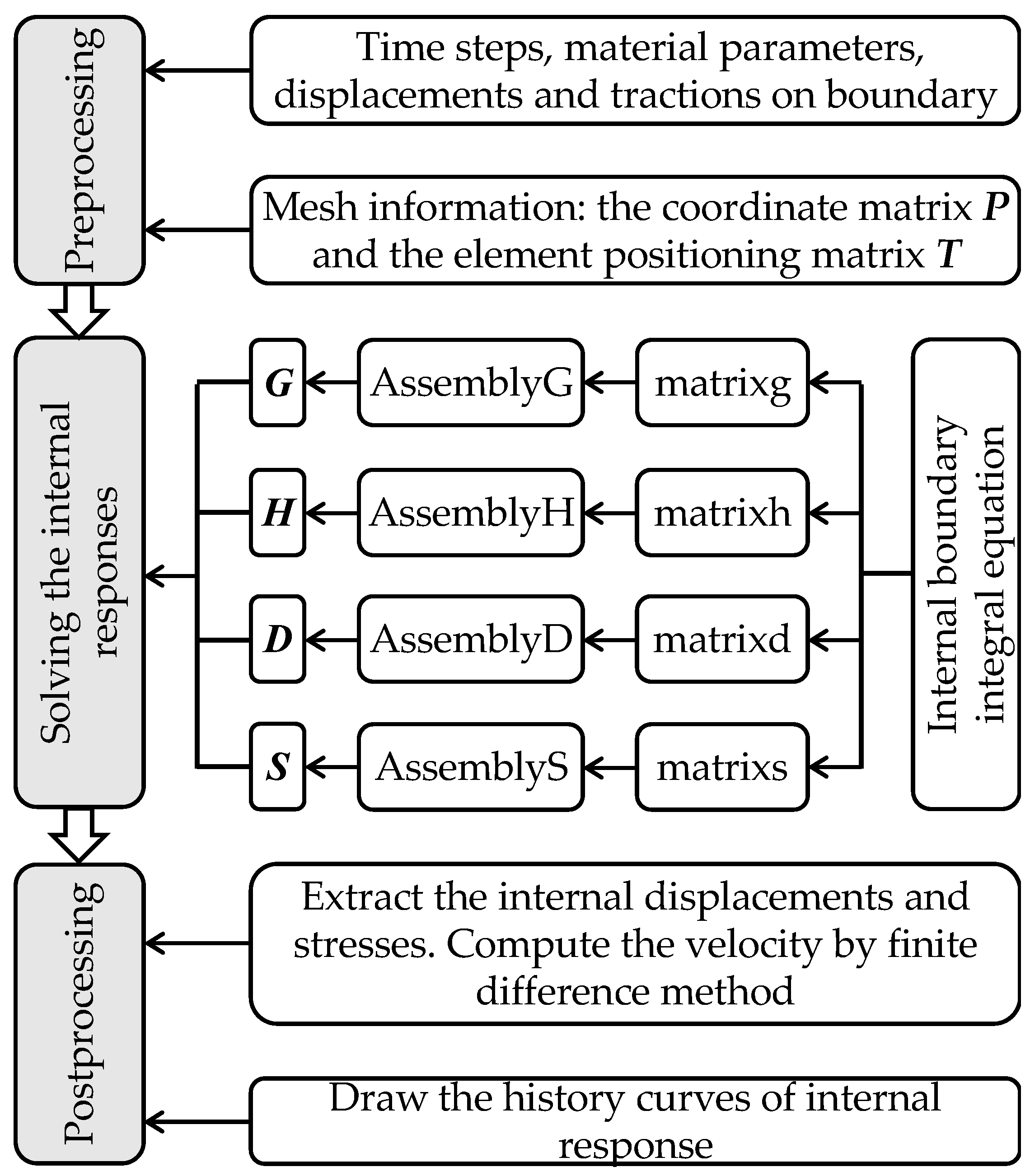
3.4. Programmatic Implementation

The theoretical framework for internal responses has been established, and the next step is its programmatic implementation. Programmatic implementation is critical in transitioning the TD-BEM from theory to practice. It validates the correctness of the theory and significantly enhances computational efficiency and practicality, thereby enabling broader application of the method in scientific research and engineering. Figure 3 illustrates the flowchart of the computational procedure. The computational procedure of the proposed algorithm is as follows:
Preprocessing: First, the material parameters, time step size, and displacements and tractions at all boundary points are input. Subsequently, mesh generation is performed to produce the nodal coordinate matrix P and the element connectivity matrix T.
Solving the internal responses: The boundary integral equations are discretized to form the element influence coefficients g, h, d, and s, which are computed using matrixg, matrixh, matrixd, and matrixs, respectively. Wavefront singularities are eliminated through an analytical approach. The computed element influence coefficients are then assembled into the global influence coefficient matrices G, H, D, and S using AssemblyG, AssemblyH, AssemblyD, and AssemblyS. These global matrices are substituted into Equations (29) and (30) to obtain the displacements and stresses at internal points.
Postprocessing: The displacements and stresses at internal points are extracted, and the internal velocities are computed using the finite difference method. Finally, the time-history curves of the internal responses are plotted.

4. Calculation of Internal Velocities Using Finite Difference Methods

The internal velocities can be obtained by applying finite difference formulas to the internal displacements computed using the TD-BEM. Therefore, the precision of the boundary nodal displacement results determines the accuracy and stability of the computed internal velocities.
v i = u i u i 1 Δ t
u i represents the displacement of the posterior node of the calculation node, u i 1 represents the displacement of the anterior node of the calculation node, and Δ t is the time step.

5. Example Verification Analysis

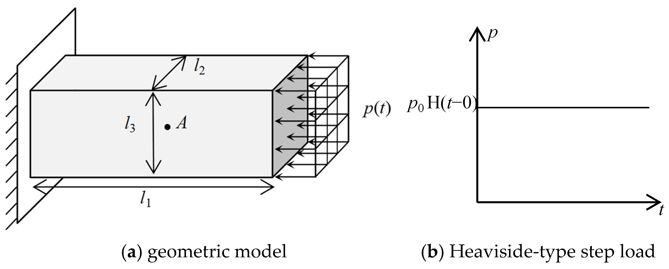
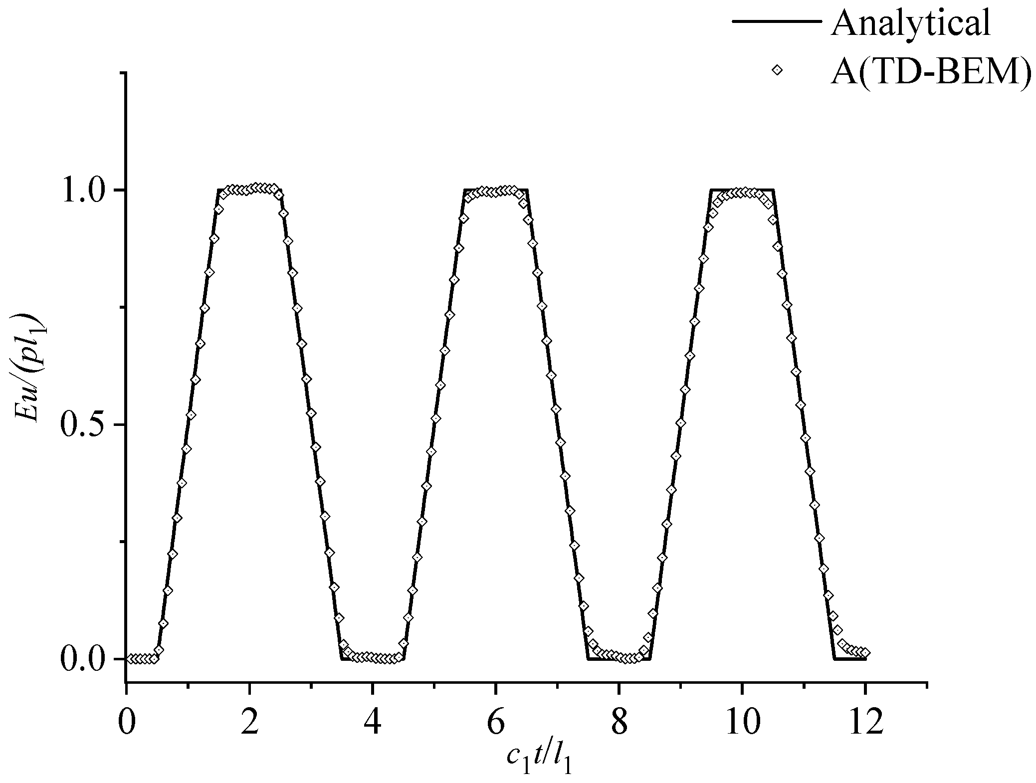
5.1. One-Dimensional Rod Example Validation Analysis

The one-dimensional rod example is a classic benchmark for validating the TD-BEM algorithm. Here, a one-dimensional rod subjected to a Heaviside-type step load is selected. Its geometric model is shown in Figure 4a, with a length l1 = 4 m and both width l2 and height l3 equal to 1 m. The left end of the rod is fixed, while the right end is subjected to a Heaviside load p = p 0 H ( t 0 ) , where the loading curve is illustrated in Figure 4b. The rod is characterized by elastic modulus E = 2.1 × 10 5 Mpa , Poisson’s ratio ν = 0 , and material density ρ = 7.9 × 10 3 kg / m 3 .
The mesh division is illustrated in Figure 5. To avoid corner point issues, linear discontinuous elements are used for mesh generation, resulting in 288 linear quadrilateral elements with a side length of 250 mm. This division also generates 1152 boundary nodes.
The calculation points are selected as A (l1/2, l2/2, l3/2). The internal stress results obtained using the TD-BEM algorithm are compared with the existing analytical solutions. Calculations were performed for three periods. Both the horizontal and vertical coordinates were dimensionless. The vertical coordinate was scaled by multiplying by 1 / p 0 , and the horizontal coordinate was scaled by multiplying by c 1 / l 1 , where p 0 represents the applied load, c 1 is the longitudinal wave speed, and l 1 is the length of the rod.
By comparing the results obtained from the TD-BEM with the analytical solutions, the computed displacement results at point A exhibit excellent agreement with the reference solution, with accurate peak values and high precision (Figure 6). Additionally, the stress results show good agreement, with precise, reasonable peak values, meeting the basic requirements (Figure 7). However, the stress curve does not fully match the sharp vertical line shape of the analytical solution. This discrepancy arises because the boundary tractions and displacements used as input for the internal stress calculations are derived from the TD-BEM displacement computation program, which may introduce cumulative errors. Insufficient precision in the boundary displacements and tractions directly affects the accuracy of the subsequent stress results.
An error analysis of the results is now conducted to validate the above statement. Ey is used to denote the error percentage, E y = y y 0 y 0 × 100 % , where y represents the TD-BEM numerical solution and y0 denotes the analytical solution. As can be observed from Table 2, the error percentages at intermediate values are slightly higher than those at the peaks but remain within an acceptable range. The correctness of the TD-BEM theory for internal responses and the feasibility of the proposed method have been validated.

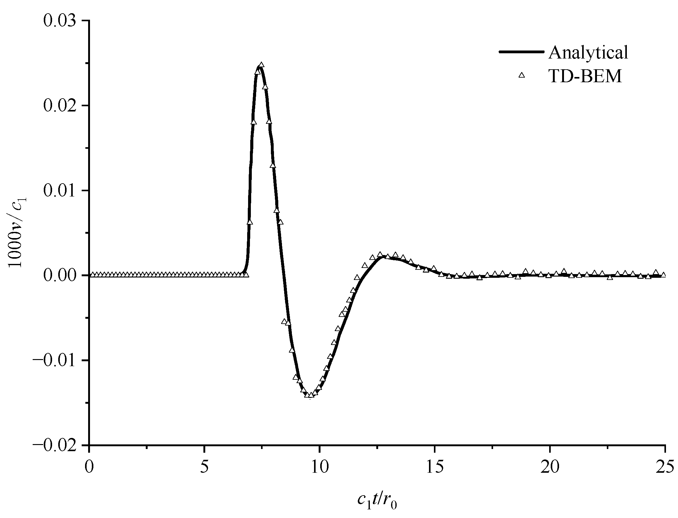
5.2. Infinite Domain with a Cavity Example Validation Analysis

The computational model comprises a spherical cavity in an infinite, homogeneous, and isotropic elastic medium. The inner radius of the cavity is r0 = 1 m. A spherical explosion load is applied along the cavity, and the expression for the explosion load is p t = k p 1 e a t e b t (k = 1.435, a = 1279 s−1, b = 12,792 s−1, p1 = 100 MPa); the time history curve is shown in Figure 8b. Poisson’s ratio ν here is set to 0.3
Boundary point A (r0, 0, 0) and an internal point (2r0, 0, 0) located 2 m from the center of the sphere within the surrounding medium are analyzed. The results obtained from the TD-BEM are compared with those from the analytical solution. Figure 9 shows the comparison of displacement results at r = 2 m under explosive load, and Figure 10 shows the comparison of velocity results. The coordinates are normalized: the horizontal coordinates are scaled by c 1 / r 0 , and the vertical coordinates in Figure 10 are scaled by 1000 / c 1 . Here, p 0 represents the magnitude of the step load, c 1 is the longitudinal wave velocity, and r0 is the inner radius of the spherical cavity.
Examining the result plots and error comparison tables shows that the image results of velocity and displacement match the analytical solution, with error percentages all within 7% (Table 3). These values fall within an acceptable range, demonstrating that the numerical results of this example are satisfactory. This example validates the correctness of the TD-BEM theory for internal responses and its applicability to infinite domain problems.

6. Conclusions

This paper presents a theoretical study of the TD-BEM for three-dimensional elastodynamic problems, focusing primarily on calculating internal unknowns. The main conclusions are as follows:
  • The displacement influence coefficient kernel function and the surface traction influence coefficient kernel function are derived, leading to the formulation of the internal stress boundary integral equation.
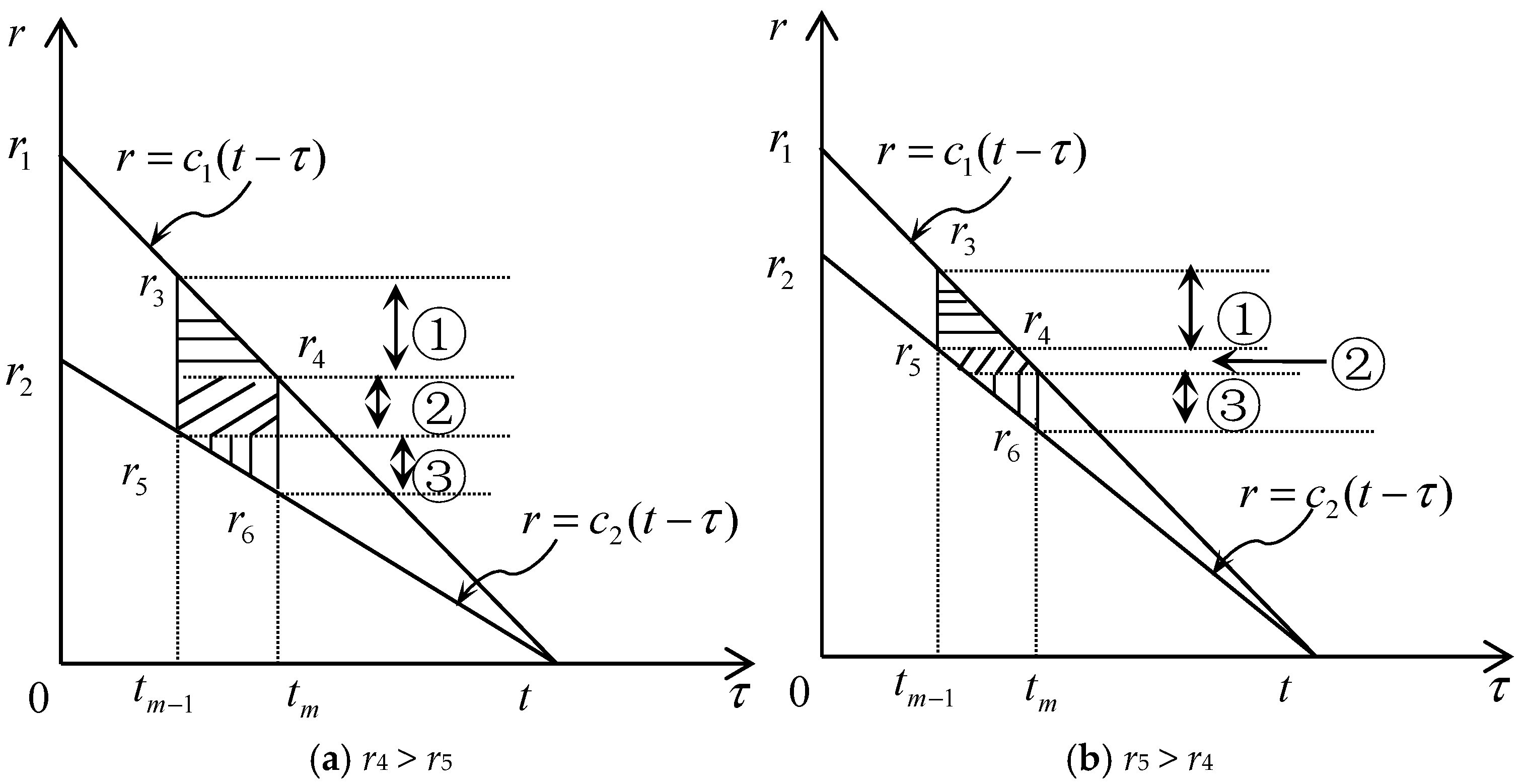
  • The singular integrals that arise, particularly those associated with the time domain wavefront singularity, are solved analytically. The values of the functions that cause the wavefront singularity are determined, focusing on solving the time integral of the second derivative of the newly introduced Dirac function.
  • The computational results show good agreement with the theoretical solution. From deriving the fundamental solution and establishing the equations to the subsequent analytical integration, all formulas and integral equations are mathematically rigorous and without any introduced errors, demonstrating that the TD-BEM is valid for solving internal stress problems.
  • This paper provides further theoretical refinement of the TD-BEM for three-dimensional elastodynamics but has not yet delved into studying three-dimensional elastoplastic dynamics. Within the existing framework of the elastodynamics TD-BEM, the incorporation of an integral plastic term involving plastic strain, along with constitutive relations, enables the solution of elastoplastic problems. The further development of elastoplastic dynamic theory will be a key focus of our team’s future research.

Author Contributions

Conceptualization, L.L and H.L; Methodology, L.L., H.L., X.Q., W.L. and Y.L.; Software, L.L., H.L. and X.Q.; Validation, L.L., H.L. and Y.L.; Writing—original draft, L.L. and H.L.; Writing—review & editing, L.L., H.L., X.Q., W.L. and Y.L.; All authors have read and agreed to the published version of the manuscript.

Funding

This research received financial support from research grants No. 12471497 provided by National Natural Science Foundation of China and No. KY-2022-014 provided by Guangzhou Metro Design and Research Institute Co., Ltd. of China.

Data Availability Statement

The data will be made available by the authors on request.

Conflicts of Interest

The authors declare no conflict of interest. The funders had no role in the design of the study; in the collection, analyses, or interpretation of data; in the writing of the manuscript; or in the decision to publish the results.

References

  1. Karabalis, D.L.; Beskos, D.E. Dynamic response of 3-D rigid surface foundations by time domain boundary element method. Earthq. Eng. Struct. Dyn. 1984, 12, 73–93. [Google Scholar]
  2. Beskos, D.E. Boundary element methods in dynamic analysis. Appl. Mech. Rev. 1997, 50, 149–197. [Google Scholar]
  3. Ahmad, S.; Banerjee, P.K. Time-domain transient elastodynamic analysis of 3-D problems by BEM. Int. J. Numer. Methods Eng. 1988, 26, 1709–1728. [Google Scholar] [CrossRef]
  4. Green, G.; Wheelhouse, T.; Lindsay, R. An essay on the application of mathematical analysis to the theories of electricity and magnetism. Phys. Today 1959, 12, 48. [Google Scholar]
  5. Kupradze, V.D.; Aleksidze, M.A. The method of functional equations for the approximate solution of certain boundary value problems. USSR Comput. Math. Math. Phys. 1964, 4, 82–126. [Google Scholar] [CrossRef]
  6. Jaswon, M.A. Integral equation methods in potential theory. Proc. R. Soc. Lond. A 1963, 275, 23–32. [Google Scholar]
  7. Brebbia, C.A. The Boundary Element Method for Engineers; Pentech Press: London, UK, 1978. [Google Scholar]
  8. Mansur, W.J.; Brebbia, C.A. Formulation of the boundary element method for transient problems governed by the scalar wave equation. Appl. Math. Model. 1982, 6, 307–311. [Google Scholar]
  9. Banerjee, P.K.; Ahmad, S.; Manolis, G.D. Transient elastodynamic analysis of three-dimensional problems by boundary element method. Earthq. Eng. Struct. Dyn. 1986, 14, 933–949. [Google Scholar]
  10. Marrero, M.; Dominguez, J. Numerical behaviour of time domain BEM for three-dimensional transient elastodynamic problems. Eng. Anal. Bound. Elem. 2003, 27, 39–48. [Google Scholar]
  11. Manolis, G.D.; Beskos, D.E. Boundary Element Methods in Elastodynamics; Unwin Hyman: London, UK, 1988. [Google Scholar]
  12. Coda, H.B.; Venturini, W.S. Three-dimensional transient BEM analysis. Comput. Struct. 1995, 56, 751–768. [Google Scholar]
  13. Hildenbrand, J.; Kuhn, G. Numerical computation of hypersingular integrals and application to the boundary integral equation for the stress tensor. Eng. Anal. Bound. Elem. 1992, 10, 209–217. [Google Scholar]
  14. Pan, E.; Yuan, F.G. Boundary element analysis of three-dimensional cracks in anisotropic solids. Int. J. Numer. Methods Eng. 2000, 48, 211–237. [Google Scholar]
  15. Panagiotopoulos, C.G.; Manolis, G.D. Three-dimensional BEM for transient elastodynamics based on the velocity reciprocal theorem. Eng. Anal. Bound. Elem. 2010, 35, 507–516. [Google Scholar]
  16. Qin, X.; Fan, Y.; Li, H.; Lei, W. A Direct Method for Solving Singular Integrals in Three-Dimensional Time-Domain Boundary Element Method for Elastodynamics. Mathematics 2022, 10, 286. [Google Scholar] [CrossRef]
  17. Lei, W.; Qin, X.; Li, H.; Fan, Y. Causality condition relevant functions-orientated analytical treatment on singularities in 3D TD-BEM. Appl. Math. Comput. 2022, 427, 127113. [Google Scholar]
  18. Pak, R.Y.S.; Guzina, B.B. Seismic soil-structure interaction analysis by direct boundary element methods—ScienceDirect. Int. J. Solids Struct. 1999, 36, 4743–4766. [Google Scholar]
  19. Pak, R.Y.S.; Bai, X.Y. A regularized boundary element formulation with weighted-collocation and higher-order projection for 3D time-domain elastodynamics. Eng. Anal. Bound. Elem. 2018, 93, 135–142. [Google Scholar]
  20. Pak, R.Y.S.; Bai, X.Y. On the stability of direct time-domain boundary element methods for elastodynamics. Eng. Anal. Bound. Elem. 2018, 96, 138–149. [Google Scholar]
  21. Israil, A.; Banerjee, P.K. Interior stress calculations in 2-d time-domain transient bem analysis. Int. J. Solids Struct. 1991, 27, 915–927. [Google Scholar]
  22. Carrer, J.A.M.; Mansur, W.J. Stress and Velocity in 2D Transient Elastodynamic Analysis by the Boundary Element Method. Eng. Anal. Bound. Elem. 1999, 23, 233–245. [Google Scholar]
  23. Schanz, M.; Antes, H. A new visco- and elastodynamic time domain boundary element formulation. Comput. Mech. 1997, 20, 452–459. [Google Scholar] [CrossRef]
  24. Antes, H.; Steinfeld, B.; Tröndle, G. Recent developments in dynamic stress analyses by time domain BEM. Eng. Anal. Bound. Elem. 1991, 8, 176–184. [Google Scholar] [CrossRef]
  25. Coda, H.B.; Venturini, W.S. Dynamic non-linear stress analysis by the mass matrix BEM. Eng. Anal. Bound. Elem. 2000, 24, 623–632. [Google Scholar] [CrossRef]
  26. Stokes, G.G. On the dynamical theory of diffraction. Trans. Camb. Philos. Soc. 1849, 9, 1–62. [Google Scholar]
  27. Love, A.E.H. A Treatise on the Mathematical Theory of Elasticity, 4th ed.; Dover: New York, NY, USA, 1944. [Google Scholar]
  28. De Hoop, A.T. Representation Theorems for the Displacement in an Elastic Solid and Their Application to Elastodynamic Diffraction Theory. Ph.D. Thesis, Delft University of Technology, Delft, The Netherlands, 1958. [Google Scholar]
  29. Payton, R.G. An application of the dynamic Betti-Rayleigh reciprocal theorem to moving point loads in elastic media. Q. Appl. Math. 1964, 21, 299–313. [Google Scholar] [CrossRef]
  30. Aliabadi, M.H. The Boundary Element Method; Wiley: New York, NY, USA, 2002; Volume 2: Applications in Solids and Structures. [Google Scholar]
Figure 1. Time space integral domain of wavefront singularity.
Mathematics 13 01025 g001
Figure 2. Division of integral region in time t m 1 , t m element.
Mathematics 13 01025 g002
Figure 3. Flowchart of the computational procedure for internal responses.
Mathematics 13 01025 g003
Figure 4. One-dimensional rod geometric model and applied load type.
Mathematics 13 01025 g004
Figure 5. Mesh generation.
Mathematics 13 01025 g005
Figure 6. Comparison diagram of displacement results of TD-BEM and analytical solution for point A.
Mathematics 13 01025 g006
Figure 7. Comparison diagram of stress results of point A TD-BEM and analytical solution.
Mathematics 13 01025 g007
Figure 8. Spherical cavity model and explosion load.
Mathematics 13 01025 g008
Figure 9. Comparison diagram of displacement results of r = 2 m TD-BEM and analytical solution under explosion load.
Mathematics 13 01025 g009
Figure 10. Comparison of velocity results of TD-BEM and characteristic line method at r = 2 m under explosion load.
Mathematics 13 01025 g010
Table 1. The result of the integration of the function causing the singularity of the wavefront on t m 1 , t m .
τ [ t m 1 , t r / c 1 ] r [ r 4 , r 3 ] τ [ t m 1 , t m ] r [ r 5 , r 4 ] τ [ t r / c 2 , t r / c 1 ] r [ r 4 , r 5 ] τ [ t r / c 2 , t m ] r [ r 6 , r 5 ]
t m 1 t m H w d τ 1 1 1 1
t m 1 t m δ c 1 f ( τ ) d τ f ( t r / c 1 ) 0 f ( t r / c 1 ) 0
t m 1 t m δ c 2 f ( τ ) d τ 00 f ( t r / c 2 ) f ( t r / c 2 )
t m 1 t m δ c 2 f ( τ ) d τ f ( t r / c 1 ) 0 f ( t r / c 1 ) 0
t m 1 t m δ c 2 f ( τ ) d τ 00 f ( t r / c 2 ) f ( t r / c 2 )
t m 1 t m δ c 1 f ( τ ) d τ f ( t r / c 1 ) 0 f ( t r / c 1 ) 0
t m 1 t m δ c 2 f ( τ ) d τ 00 f ( t r / c 2 ) f ( t r / c 2 )
Table 2. Errors comparison of the one-dimensional rod example results.
Number   c 1 t / l 1 σ x / p 0
TD-BEM
σ x / p 0 AnalyticalError Percentage E u / p l 1
TD-BEM
E u / p l 1 AnalyticalError Percentage
(1) 1.01251.068216.82%0.52040.512.03%
(2) 2.02501.952722.36%1.002510.25%
(3) 2.98121.023512.35%0.52380.512.71%
(4) 5.06251.048714.87%0.65770.651.18%
(5) 6.01871.935023.25%0.997910.21%
(6) 6.9751.016411.64%0.53290.522.48%
(7) 9.05621.055315.53%0.57450.562.58%
(8) 10.01251.938723.06%0.995910.41%
(9) 10.96871.020112.01%0.54190.532.24%
Table 3. Errors comparison of the infinite domain with the cavity example results.
Number   c 1 t / r 0 u TD-BEM u AnalyticalError Percentage Number   c 1 t / r 0 1000 v / c 1 TD-BEM 1000 v / c 1 Error Percentage
(1) 7.64390.01210.01296.2%(1) 7.14540.01790.01895.29%
(2) 8.47480.02320.02205.45%(2) 7.47770.02470.02393.34%
(3) 9.63800.01120.01185.08%(3) 7.97620.01280.01290.77%
(4) 5.0625−0.0057−0.00553.63%(4) 9.638−0.0141−0.01451.02%
(5) 13.2938−0.0032−0.00306.89%(5) 10.4688−0.0095−0.01026.86%
Disclaimer/Publisher’s Note: The statements, opinions and data contained in all publications are solely those of the individual author(s) and contributor(s) and not of MDPI and/or the editor(s). MDPI and/or the editor(s) disclaim responsibility for any injury to people or property resulting from any ideas, methods, instructions or products referred to in the content.

