Abstract
With the increasing prevalence of intermittent power generation, the volatility, intermittency, and randomness of renewable energy pose significant challenges to the planning and operation of distribution networks. In this study, a data-driven distributionally robust optimization model is introduced. This model takes into account the forecasting errors of wind power generation, as well as the operational constraints and coordinated control of energy storage, demand-side loads, and conventional generating units. The model can obtain the scheduling scheme with the lowest cost in scenarios with uncertain wind power. Unlike traditional stochastic methods, this model uses the Wasserstein metric to construct the uncertainty set from wind power big data without the need to pre-determine the probability distribution or distribution interval of errors. This is achieved through a Wasserstein ball centered on empirical distribution. As the amount of historical data grows, the model adjusts the radius of the Wasserstein ball, thus reducing the conservatism of the results. Compared with traditional robust optimization methods, this system can achieve lower operating costs. Compared with traditional stochastic programming methods, this system has higher reliability. Finally, the superiority of the proposed model over traditional models is verified through simulation analysis.
MSC:
90C29
1. Introduction
With the continuous increase in the penetration rate of renewable energy sources in the power system, the uncertainties associated with renewable energy can no longer be overlooked and pose significant risks to the security of the power system. Managing these risks has been recognized as a major challenge [1,2]. A direct approach to addressing this issue is to add extra reserve capacity, which means installing and using more conventional generators (CGs) to ensure the robustness of the power system in the face of uncertainties. However, this method is inefficient and highly dependent on the practical experience of operators. As a result, it is difficult to guarantee that the system will not face capacity shortages during load variations [3,4]. Therefore, it is of great significance to develop optimization models and corresponding solutions that take into account the uncertainties of renewable energy sources for the reliable and cost-effective operation of the power system. The most commonly used techniques for managing uncertainties in power systems are robust optimization (RO) and stochastic programming (SP), but both of them have significant limitations in balancing computational efficiency, economic efficiency, and robustness [5,6].
Stochastic programming is an uncertainty analysis technique based on probability theory, and its effectiveness relies on the prior assumption of the precise probability distribution of uncertain parameters [7,8,9] or a large number of scenarios [10,11]. This inevitably leads to an increase in computational burden and problem complexity [12]. Although scenario reduction techniques can partially alleviate the computational burden [13], due to the high sensitivity of economic dispatch decisions to the accuracy of renewable energy generation scenario modeling, a delicate trade-off between the typicality and extremity of scenarios is required during the scenario reduction process. However, the balancing ability of existing methods in this regard still needs in-depth research. In addition, reference [14] proposed an adaptive stochastic optimization algorithm that integrates uncertain loads and electricity price fluctuations. Although this stochastic method provides probabilistic guarantees for meeting constraints, using deterministic probability curves to describe the uncertain changes in stochastic parameters may not accurately reflect the real conditions.
The robust optimization method addresses parameter fluctuations by constructing an uncertainty set, ensuring that feasible solutions remain valid when parameters vary within this set [15]. This method has been widely applied in the field of energy optimization. For example, [16] uses an uncertainty budget to minimize the total cost under the worst-case wind power generation scenario [17], combines robust optimization with piecewise linearization for microgrid energy storage dispatch, [18] introduces a versatile uncertainty set to handle fluctuating wind power output, etc. However, all these methods have a key drawback. Traditional uncertainty sets are usually too conservative. They ignore the available probability information and sacrifice economic efficiency in exchange for robustness guarantees in extreme scenarios.
Distributionally robust optimization (DRO) has received extensive attention in recent years because it combines the complementary advantages of SP and RO. Unlike stochastic programming, DRO constructs an ambiguity set containing all possible distributions through historical data and solves for the optimal decision under the worst-case distribution, thus avoiding the dependence on the precise probability distribution and addressing the shortcoming of traditional robust optimization methods that ignore probability information. Existing methods for constructing ambiguity sets mainly include three categories: moment-based methods [19,20], cumulative distribution function-based methods [21], and Kullback–Leibler (KL) divergence-based methods [22]. Although the above methods can effectively represent uncertainties, they still have the following limitations: (1) the moment-based method cannot guarantee that the ambiguity set will converge to the true distribution as the amount of data increases; that is, there is still room for improvement in terms of economic efficiency; (2) the cumulative distribution function-based method results in relatively high conservatism due to the neglect of the joint distribution information between the empirical distribution and the true distribution; (3) the KL divergence-based model is difficult to solve with conventional optimization tools due to the nonlinearity of the objective function.
To address the above issues, this paper proposes a distributionally robust optimization model based on the Wasserstein metric. The model defines the ambiguity set by constructing a Wasserstein ball centered on empirical distribution, and experiments show that when the amount of historical data increases, the empirical distribution will asymptotically converge to the true distribution. Compared with the moment-based method and the cumulative distribution function-based method, the proposed method reduces the conservatism of the results by making more effective use of historical data. Compared with the KL divergence-based method, its characteristics make it more convenient to use conventional algorithms such as column generation and constraint generation (C&CG) for efficient solutions. The main contributions of this paper are outlined as follows:
- (1)
- A structural model for a microgrid that incorporates wind energy, energy storage, and demand response load is proposed, accounting for the uncertainty in the power generated by wind turbines. Energy storage is employed to enhance the grid’s capability to accommodate wind power.
- (2)
- We utilize the Wasserstein metric to construct the uncertainty set for wind power. Increasing the volume of historical data leads to a gradual convergence of the empirical distribution towards the true distribution. This convergence mitigates the conservatism of optimal decisions, thereby achieving more optimal operational costs while adhering to equipment constraints.
- (3)
- To address the optimization and scheduling challenges of the aforementioned microgrid, a two-stage RO approach is employed. This method offers increased flexibility compared to traditional single-stage RO.
The rest of this paper is organized as follows: Section 2 establishes the model of the microgrid and describes in detail the cost functions and constraint conditions of each part in the microgrid; Section 3 constructs the ambiguity set of wind energy prediction errors using the Wasserstein metric; Section 4 presents the solution method for the proposed optimization model; Section 5 verifies the effectiveness of the proposed model through numerical results, compares it with traditional robust optimization and stochastic programming models, and demonstrates its ability to balance economic efficiency and robustness. Section 6 concludes the full text.
2. Microgrid Modeling
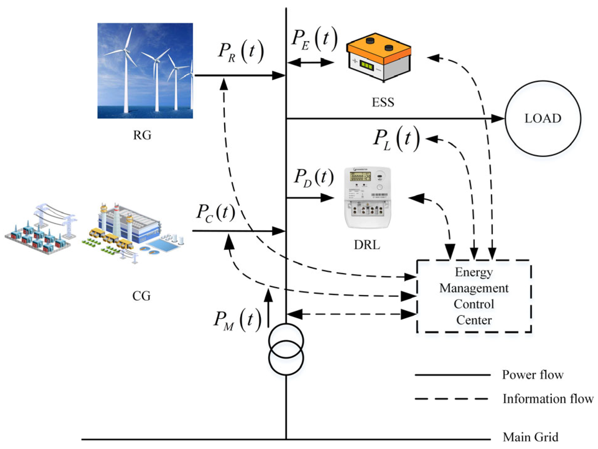
A typical grid-connected microgrid is structured as shown in Figure 1, which includes components such as renewable generators (RGs), energy storage systems (ESSs), conventional generators (CGs), conventional loads, and demand response (DR) loads. Moreover, the microgrid is connected to the main grid, enabling electricity transactions. All these components are centrally controlled by the energy management control center.
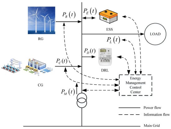
Figure 1.
Microgrid structure with RG, CG, ESS, and load.
The power balance relationships among the components are as follows:
where represents the power exchanged between the microgrid and the main grid, which is measured on the microgrid side. When , it indicates that the main grid supplies power to the microgrid; when , it means that the microgrid exports power to the main grid. denotes the power demand of the conventional load, represents the DR loads, is the output power of the conventional power generation system, and is the output power of the renewable energy power generation system (in this paper, the renewable energy is wind energy). stands for the charging/discharging power of the energy storage system measured on the AC side. Specifically, when , the energy storage system is charging; when , the energy storage system is discharging. Subsequently, each part of the system will be explained in detail block by block.
2.1. Electricity Transaction Cost
When operating in grid-connected mode, the microgrid balances supply and demand by conducting power transactions with the main grid, thereby optimizing operational efficiency. During time period , the scale and direction of power exchange are influenced by the electricity prices in the same period. Considering that electricity is typically prioritized for areas experiencing shortages, it can be assumed that during period , the price for selling electricity is not higher than the cost of purchasing it.
As shown below, the electricity transaction cost is defined by the total expenditures and revenues generated through the power exchange between the microgrid and the main grid.
where , are the power purchasing and selling prices within the time period , and and are the parameters representing the power purchasing or selling status of the microgrid. When , signifies that electricity is being purchased from the main grid, and when , indicates that electricity is being sold to the main grid. and satisfy the following constraints:
In addition, the exchange power is subject to the following constraints:
where and represent the upper limits of the exchange power and the exchange power change rate, respectively.
2.2. Demand Response Load
The incentive mechanism of the DR program in this paper is designed by referring to the relevant content in [23]. Specifically, the DR program is implemented through incentive measures. When the grid load is too high or there is a need to balance the power supply, if users can shift their electricity loads, they will receive a certain economic compensation.
The scheduling cost of the DR load in the microgrid can be represented by the following equation:
where represents the scheduling cost coefficient of the DR loads, and denotes the expected power consumption of the DR load during time period .
Under normal circumstances, users adjust their electricity usage patterns based on subsidy policies, shifting some of their electricity demand to other time periods. Direct changes in electricity consumption are rare, and users have limited ability to adjust their power demand. Therefore, the following constraints need to be added: when adjusting demand response loads, the total electricity demand must remain unchanged, and the electricity demand in each time period must be within specified upper and lower limits.
where is the total energy demand of the DR load within the scheduling period; and and are the minimum and maximum energy demand of the DR load during time period , respectively.
The absolute value term in (8) represents the difference between the actual dispatched power and the anticipated power consumption. By introducing auxiliary variables and and constraints (12) and (13), (8) can be linearized as shown in (b11):
2.3. Conventional Generator
The main forms of CG units are micro-turbines (MT) and fuel cells, and their power generation costs can be represented by a linear function. In this paper, we consider the case where the CG units are composed of MT. The cost function and the start-up cost function are as follows:
where and are cost coefficients, represents the unit start-up cost coefficient, and represents the state of the equipment, which satisfies the following constraints:
when , it means that the unit is in the working state, and when , it means that the unit is not in the working state.
During each time interval , CG units must meet the power output and ramp rate constraints shown below.
where and represent the minimum and maximum output powers of the MT, respectively, and and represent the lower and upper limits of the power change rate of the MT, respectively.
2.4. Energy Storage System
In a microgrid, ESS units can have various forms such as batteries, liquid air, and flywheels. Owing to their extensive application and high charge/discharge efficiency, the ESS in this paper is made up of Li-ion batteries.
The maintenance expense of the ESS during time period is expressed as:
where represents the operation cost coefficient of the ESS.
Let represent the energy stored in the ESS during time period . Then, when the ESS is charging and discharging, we have the following, respectively:
where and represent the charging and discharging efficiencies of the energy storage system, respectively, which are defined as the efficiency of electrical energy conversion during the charging and discharging processes of the energy storage system.
Since the energy storage system needs to meet the maximum and minimum capacity limits , we have:
Meanwhile, in order to prevent the charging and discharging power from being too large, the power constraints need to be satisfied:
where , , , and represent the maximum and minimum values of the energy stored in the ESS and the maximum charging and discharging powers of the ESS, respectively.
Additionally, for the periodically operated ESS, within one cycle, the capacity at the final time should be equal to the capacity at the initial time, which can be expressed as:
3. Uncertainty of RG
In this section, we construct an ambiguity set using the Wasserstein metric, which encompasses the true probability distribution of wind power forecast errors. The uncertainty in wind power is described through this ambiguity set.
3.1. Wasserstein Metric
To determine the optimal scheduling strategy for the microgrid, it is crucial to understand the probability distribution of wind. However, in reality, there are only limited historical data, making it impossible to derive an exact probability distribution. Therefore, based on the finite samples , we can only obtain an observed distribution , which approximates the real distribution. Based on this empirical distribution, we construct an ambiguity set that aims to include the real distribution to the greatest extent possible. Additionally, as the number of samples increases, the empirical distribution converges to the real distribution, and the elements within the ambiguity set should also gradually converge to the empirical distribution to reduce conservatism.
Given the compact support space , the Wasserstein metric for the probability distributions and is defined as:
where represents the set of all the probability distributions. is a random variable with distribution . denotes the distance between the random variables. is a joint distribution of and . Consequently, the ambiguity set is defined as:
Note that represents a Wasserstein ball with the radius of and centered at . The parameter significantly influences the performance of the robust model based on the Wasserstein metric. In accordance with the aforementioned requirements, to ensure that the ambiguity set exhibits convergence properties, can be defined as:
where is a confidence level, and is the diameter of the support . can be obtained by solving the optimization problem (27):
where is a positive number, and is the sample mean. Further explanations of the above formula can be found in [24].
3.2. Uncertainty Sets
The uncertainty set , being a subset of , has a significant impact on the convergence of the ambiguity set. Given the point forecast value and the forecast error probability density function for the forecast error, the uncertainty set can be defined by:
where and are determined by an appropriate confidence level.
For RG, utilizing the base forecast value and the chosen forecast error probability density function , according to (28), the lower and upper bounds can be derived by:
Due to the power constraint bounds calculated from (29) and (30) potentially violating the original output power limits of the RG unit, it is necessary to adjust the output power limits as follows:
Therefore, according to (31) and (32), the uncertain set can be defined as:
Further explanations of the above formula can be found in [25,26].
4. Energy Management Optimization
This paper assumes that all renewable energy sources are prioritized in dispatch, with any surplus used for charging the ESS. To determine a set of appropriate operating points for distributed resources, ensuring that power dispatch meets specific demands and achieves maximum benefits, we propose an energy management model for grid-connected microgrids, as shown below:
where
The two-stage RO model constructed in this article aims to find the most economically optimal scheduling solution for uncertain variables changing to the worst-case scenario within the uncertain set . In (34), the minimization of the outer layer constitutes the problem of the first stage, with the optimization variable being the on/off status of CGs. The max-min problem within the inner layer constitutes the second stage problem, and , and are the optimization variables. denotes the uncertainty of RG, denotes the scheduling results for the CG, ESS, and main grid. represents the optimization variable given a set of . The specific expression is as follows:
where , , , and represent the dual variables associated with each constraint in the second-stage minimization problem. For the two-stage RO model mentioned above in (34), this paper employs the column-and-constraint generation (C&CG) algorithm for solving, as documented in [18]. Similar to the Benders decomposition algorithm, the C&CG algorithm also iteratively solves the original problem by decomposing it into a master problem and sub-problems. The distinction is that the C&CG algorithm continually adds variables and constraints associated with the sub-problems during the solution process of the master problem. This allows for obtaining a more compact lower bound on the original objective function, effectively reducing the number of iterations. After decomposing (34), the master problem takes the form as below:
where is the current iteration number, is the solution to the sub-problem after the l-th iteration, and is the value of the uncertain variable obtained after the l-th iteration under the worst-case scenario.
The decomposed form of the sub-problem is:
Based on the analysis provided earlier, it is known that under the given , the inner minimization problem in (37) is a linear problem. According to the strong duality theory and the correspondence of (35), it can be transformed into a max problem. By combining it with the outer maximization problem, the dual problem is derived as follows:
After the aforementioned derivation and transformation, the two-stage robust model is ultimately decoupled into the main problem, denoted as (36), and the sub-problem, denoted as Equation (38), both in mixed-integer linear form. Subsequently, it can be solved using the C&CG algorithm. The process is as follows:
Step 1: Given a set of values for the uncertain variable as the initial worst-case scenario, set the lower bound and upper bound for the operating cost corresponding to the final scheduling plan. Initialize the iteration count as ;
Step 2: Based on the worst-case scenario , solve the main problem given by (36) to obtain the optimal solution . The objective function value of the main problem serves as the new lower bound ;
Step 3: Substitute the obtained solution for the main problem into (38), solve the sub-problem, and obtain the objective function value of the sub-problem along with the corresponding values of uncertain variables under the worst-case scenario. Update the upper bound based on these results;
Step 4: Given a convergence threshold for the algorithm, if , stop the iteration and return the optimal solutions and ; Otherwise, add the variable and add the following constraints:
Step 5: Let , proceed to Step 2, and continue the algorithm iterations until convergence.
5. Experiment Validation and Discussion
In this section, we provide numerical results for a microgrid system that includes CGs, wind turbines, energy storage systems, conventional loads, and DR loads to validate the accuracy of the theoretical outcomes. The prediction and historical data of the wind farm are based on the typical day-ahead prediction errors reported in an American study [27]. The day-ahead trading prices for power exchanges between the microgrid and the main grid are illustrated in Figure 2, and the demand profile of the regular loads is presented in Figure 3.
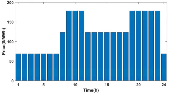
Figure 2.
Day-ahead trading prices for power exchanges.
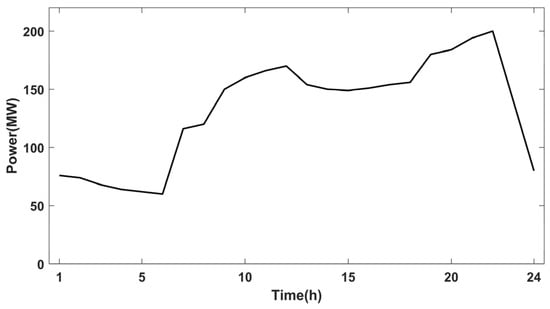
Figure 3.
Demand profile of the regular loads.
The microgrid’s operating parameters are presented in Table 1.

Table 1.
Operation parameters of microgrid.
5.1. Economic Dispatch Scheme of Microgrid
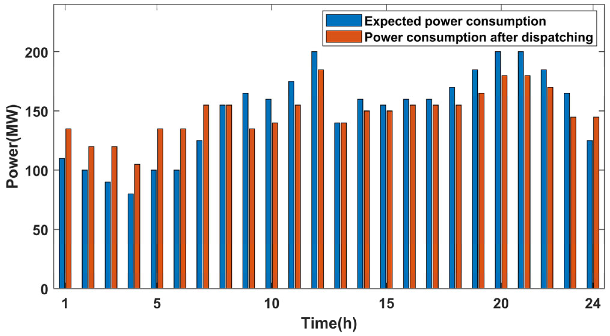
First, a set of wind power data is randomly selected from the historical dataset to demonstrate the system’s optimal scheduling process. The microgrid scheduling optimization results are shown in Figure 4 and Figure 5. As seen in Figure 4, the energy storage unit charges between 2 and 8 h and at 10 h and discharges from 19 to 23 h. Combined with Figure 2, it can be observed that when the electricity selling price is low, the energy storage system stores electrical energy, and when the price is high, it releases energy, thus achieving peak shaving and valley filling while maximizing economic benefits. Figure 5 shows that the microgrid reallocates the high peak electricity demand originally occurring from 9 to 12 h and 14 to 23 h to 1 to 7 h and 24 h. In combination with Figure 3, it can be seen that before the adjustment, the power demand was primarily concentrated during high-electricity-price periods; after the adjustment, a portion of the demand during these periods has been shifted to periods with lower electricity prices, further enhancing the economic benefits.
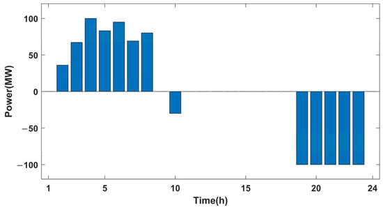
Figure 4.
Charge/discharge power of ESS.

Figure 5.
Expected power consumption and power consumption after dispatching.
5.2. Robustness Verification
When the number of historical samples is small, the empirical distribution obtained from historical samples may significantly differ from the actual distribution. To ensure that the real distribution is contained within the ambiguity set, a larger radius of the Wasserstein ball is required, resulting in a more conservative ambiguity set. As the volume of historical data grows, the observed distribution progressively converges towards the true distribution. Consequently, the radius of the Wasserstein ball can be reduced while still containing the real distribution within the ambiguity set. Reducing the radius of the Wasserstein ball decreases the conservatism of the solution. The radius of the Wasserstein ball derived from historical data is shown in Table 2. It is evident that with more historical samples, the radius of the Wasserstein ball steadily shrinks, indicating that the uncertainty set becomes smaller.
Table 2.
Wasserstein ball radius and bounds under various sample sizes.
5.3. Comparative Analysis with RO and SP
In this section, we evaluate the cost-effectiveness and reliability of the proposed DRO model by comparing it with the SP model based on the Gaussian distribution and the RO model described in reference [28]. Using real historical data, we conduct 10,000 Monte Carlo simulations for the SP model, the RO model, and the DRO model with different dataset scales. The results are shown in Table 3, Table 4 and Table 5. It is observed that as the number of historical samples increases, the cost of the proposed model decreases. When the sample size is small, the empirical distribution may significantly differ from the real distribution. To ensure system robustness, the proposed model adopts a more conservative scheduling strategy, similar to that of the RO model. As a result, its average cost is close to that of the RO model. Conversely, when the historical dataset is large, the empirical distribution is closer to the real distribution, allowing the proposed model to adopt a more aggressive scheduling strategy similar to that of the SP model, thereby reducing the cost. Meanwhile, as shown in Table 3, the feasibility probability of the proposed model decreases slightly with increasing sample size but remains above 99%, demonstrating high reliability. These results indicate that, based on the number of samples, the proposed model can balance economic efficiency and robustness, and shows better performance in terms of economy and robustness compared with the RO and SP models, respectively.
Table 3.
Monte Carlo simulation results of the proposed DRO model.
Table 4.
Monte Carlo simulation results of the RO model.
Table 5.
Monte Carlo simulation results of the SP model.
6. Conclusions
In this paper, a novel data-driven distributionally robust energy management framework for microgrids is proposed. This framework utilizes the Wasserstein metric to construct an ambiguity set based on historical wind power data. Our approach integrates the coordinated scheduling of CGs, ESS, and DR loads, enabling a balance to be struck between economic efficiency and robustness. Simulation results show that the operating costs obtained by our framework consistently fall between those of traditional robust optimization methods and stochastic programming methods. As the number of historical samples increases, the empirical distribution converges towards the true distribution, gradually reducing the conservatism of system decisions. Consequently, economic efficiency is effectively improved. Moreover, according to the experiments, it can be found that during this process, the system always maintains good reliability.
However, our study still has some limitations. First, the model fully leverages historical data, which avoids sacrificing the economic efficiency of the vast majority of regular scenarios due to a few extreme events, but it may lead to suboptimal performance when facing extreme events that are rare or absent in the historical record—an inherent issue in all data-driven approaches. Second, some of the model parameters are selected based on empirical experience, which makes it difficult to achieve optimal performance. Addressing these issues is of significant importance for practical deployment.
Overall, the main contribution of this work lies in developing a data-driven framework that effectively balances robustness and economic efficiency in microgrid energy management. We believe that the results of this study lay a solid foundation for future research. In subsequent work, we plan to incorporate quantitative risk assessment metrics and explore more advanced parameter optimization techniques to further enhance model performance and better handle extreme, low-probability events.
Author Contributions
Z.W.: methodology, writing—original draft. R.C.: writing—review and revision of the original draft. D.T.: data curation, visualization, formal analysis. C.W.: conceptualization, resources. X.L.: software, validation. W.H.: writing—review and editing, data curation. All authors have read and agreed to the published version of the manuscript.
Funding
This research was funded by the National Natural Science Foundation of China (NNSF) (Grant No. 62103443), Hunan Natural Science Foundation (Grant No. 2022JJ40630), Graduate Students Explore Innovative Projects of Central South University (Grant No. 2024ZZTS0794).
Data Availability Statement
The original contributions of the study are included in the article. Requests for additional information can be directed to the corresponding author.
Conflicts of Interest
Rui Cao was employed by Aluminum Corporation of China Ningxia Energy Group Co., Ltd. The remaining authors declare that the research was conducted in the absence of any commercial or financial relationships that could be construed as a potential conflict of interest.
References
- Zahedi, A. A Review of Drivers, Benefits, and Challenges in Integrating Renewable Energy Sources into Electricity Grid. Renew. Sustain. Energy Rev. 2011, 15, 4775–4779. [Google Scholar] [CrossRef]
- Lei, B.; Ren, Y.; Luan, H.; Dong, R.; Wang, X.; Liao, J.; Fang, S.; Gao, K. A Review of Optimization for System Reliability of Microgrid. Mathematics 2023, 11, 822. [Google Scholar] [CrossRef]
- Bertsimas, D.; Litvinov, E.; Sun, X.A.; Zhao, J.; Zheng, T. Adaptive Robust Optimization for the Security Constrained Unit Commitment Problem. IEEE Trans. Power Syst. 2013, 28, 52–63. [Google Scholar] [CrossRef]
- Ali, Z.M.; Diaaeldin, I.M.; H. E. Abdel Aleem, S.; El-Rafei, A.; Abdelaziz, A.Y.; Jurado, F. Scenario-Based Network Reconfiguration and Renewable Energy Resources Integration in Large-Scale Distribution Systems Considering Parameters Uncertainty. Mathematics 2021, 9, 26. [Google Scholar] [CrossRef]
- Fazlalipour, P.; Ehsan, M.; Mohammadi-Ivatloo, B. Risk-Aware Stochastic Bidding Strategy of Renewable Micro-Grids in Day-Ahead and Real-Time Markets. Energy 2019, 171, 689–700. [Google Scholar] [CrossRef]
- Gómez Sánchez, M.; Macia, Y.M.; Fernández Gil, A.; Castro, C.; Nuñez González, S.M.; Pedrera Yanes, J. A Mathematical Model for the Optimization of Renewable Energy Systems. Mathematics 2021, 9, 39. [Google Scholar] [CrossRef]
- Wang, Q.; Guan, Y.; Wang, J. A Chance-Constrained Two-Stage Stochastic Program for Unit Commitment With Uncertain Wind Power Output. IEEE Trans. Power Syst. 2012, 27, 206–215. [Google Scholar] [CrossRef]
- Ozturk, U.A.; Mazumdar, M.; Norman, B.A. A Solution to the Stochastic Unit Commitment Problem Using Chance Constrained Programming. IEEE Trans. Power Syst. 2004, 19, 1589–1598. [Google Scholar] [CrossRef]
- Zhao, C.; Wang, Q.; Wang, J.; Guan, Y. Expected Value and Chance Constrained Stochastic Unit Commitment Ensuring Wind Power Utilization. IEEE Trans. Power Syst. 2014, 29, 2696–2705. [Google Scholar] [CrossRef]
- Quan, H.; Srinivasan, D.; Khambadkone, A.M.; Khosravi, A. A Computational Framework for Uncertainty Integration in Stochastic Unit Commitment with Intermittent Renewable Energy Sources. Appl. Energy 2015, 152, 71–82. [Google Scholar] [CrossRef]
- Karami, M.; Shayanfar, H.A.; Aghaei, J.; Ahmadi, A. Scenario-Based Security-Constrained Hydrothermal Coordination with Volatile Wind Power Generation. Renew. Sustain. Energy Rev. 2013, 28, 726–737. [Google Scholar] [CrossRef]
- Zheng, Q.P.; Wang, J.; Liu, A.L. Stochastic Optimization for Unit Commitment—A Review. IEEE Trans. Power Syst. 2015, 30, 1913–1924. [Google Scholar] [CrossRef]
- Lorca, Á.; Sun, X.A. Adaptive Robust Optimization With Dynamic Uncertainty Sets for Multi-Period Economic Dispatch Under Significant Wind. IEEE Trans. Power Syst. 2015, 30, 1702–1713. [Google Scholar] [CrossRef]
- Dashtdar, M.; Flah, A.; Hosseinimoghadam, S.M.S.; Zangoui Fard, M.; Dashtdar, M. Optimization of Microgrid Operation Based on Two-Level Probabilistic Scheduling with Benders Decomposition. Electr. Eng. 2022, 104, 3225–3239. [Google Scholar] [CrossRef]
- Jabr, R.A.; Karaki, S.; Korbane, J.A. Robust Multi-Period OPF With Storage and Renewables. IEEE Trans. Power Syst. 2015, 30, 2790–2799. [Google Scholar] [CrossRef]
- Ju, C.; Ding, T.; Jia, W.; Mu, C.; Zhang, H.; Sun, Y. Two-Stage Robust Unit Commitment with the Cascade Hydropower Stations Retrofitted with Pump Stations. Appl. Energy 2023, 334, 120675. [Google Scholar] [CrossRef]
- Choi, J.; Shin, Y.; Choi, M.; Park, W.-K.; Lee, I.-W. Robust Control of a Microgrid Energy Storage System Using Various Approaches. IEEE Trans. Smart Grid 2019, 10, 2702–2712. [Google Scholar] [CrossRef]
- Shao, C.; Wang, X.; Shahidehpour, M.; Wang, X.; Wang, B. Security-Constrained Unit Commitment With Flexible Uncertainty Set for Variable Wind Power. IEEE Trans. Sustain. Energy 2017, 8, 1237–1246. [Google Scholar] [CrossRef]
- Wei, W.; Wang, J.; Mei, S. Dispatchability Maximization for Co-Optimized Energy and Reserve Dispatch With Explicit Reliability Guarantee. IEEE Trans. Power Syst. 2016, 31, 3276–3288. [Google Scholar] [CrossRef]
- Zhang, Y.; Shen, S.; Mathieu, J.L. Distributionally Robust Chance-Constrained Optimal Power Flow With Uncertain Renewables and Uncertain Reserves Provided by Loads. IEEE Trans. Power Syst. 2017, 32, 1378–1388. [Google Scholar] [CrossRef]
- Duan, C.; Jiang, L.; Fang, W.; Liu, J. Data-Driven Affinely Adjustable Distributionally Robust Unit Commitment. IEEE Trans. Power Syst. 2018, 33, 1385–1398. [Google Scholar] [CrossRef]
- Duan, C.; Jiang, L.; Fang, W.; Liu, J.; Liu, S. Data-Driven Distributionally Robust Energy-Reserve-Storage Dispatch. IEEE Trans. Ind. Inform. 2018, 14, 2826–2836. [Google Scholar] [CrossRef]
- Yixin, L.; Guo, L.; Wang, C. Economic Dispatch of Microgrid Based on Two Stage Robust Optimization. Proc. CSEE 2018, 38, 4013–4022. [Google Scholar]
- Duan, C. Distributionally Robust and Structure Exploiting Algorithms for Power System Optimization Problems. Ph.D. Thesis, The University of Liverpool, Liverpool, UK, 2018. [Google Scholar]
- Xiang, Y.; Liu, J.; Liu, Y. Robust Energy Management of Microgrid With Uncertain Renewable Generation and Load. IEEE Trans. Smart Grid 2016, 7, 1034–1043. [Google Scholar] [CrossRef]
- Zhang, W.; Peng, Z.; Wang, Q.; Qi, W.; Ge, Y. Optimal Power Flow Method with Consideration of Uncertainty Sources of Renewable Energy and Demand Response. Front. Energy Res. 2024, 12, 1421277. [Google Scholar] [CrossRef]
- Hodge, B.-M.; Lew, D.; Milligan, M.; Gómez-Lázaro, E.; Larsén, X.G.; Giebel, G.; Holttinen, H.; Sillanpää, S.; Scharff, R.; Söder, L.; et al. Wind Power Forecasting Error Distributions: An International Comparison. In Proceedings of the 11th International Workshop on Large-Scale Integration of Wind Power into Power Systems 2012, Lisbon, Portugal, 13–15 November 2012. [Google Scholar]
- Peng, C.; Xie, P.; Pan, L.; Yu, R. Flexible Robust Optimization Dispatch for Hybrid Wind/Photovoltaic/Hydro/Thermal Power System. IEEE Trans. Smart Grid 2016, 7, 751–762. [Google Scholar] [CrossRef]


Disclaimer/Publisher’s Note: The statements, opinions and data contained in all publications are solely those of the individual author(s) and contributor(s) and not of MDPI and/or the editor(s). MDPI and/or the editor(s) disclaim responsibility for any injury to people or property resulting from any ideas, methods, instructions or products referred to in the content. |
© 2025 by the authors. Licensee MDPI, Basel, Switzerland. This article is an open access article distributed under the terms and conditions of the Creative Commons Attribution (CC BY) license (https://creativecommons.org/licenses/by/4.0/).