Article

Generalized Cardinal Polishing Splines Signal Reconstruction

1
School of Computer Science and Engineering, Macau University of Science and Technology, Taipa, Macau 999078, China
2
Zhuhai MUST Science and Technology Research Institute, Zhuhai 519099, China
*
Author to whom correspondence should be addressed.
Mathematics 2025, 13(6), 983; https://doi.org/10.3390/math13060983
Submission received: 6 January 2025 / Revised: 8 March 2025 / Accepted: 12 March 2025 / Published: 17 March 2025
(This article belongs to the Section E1: Mathematics and Computer Science)

Abstract

:
Sampling and reconstruction are indispensable processes in signal processing, and appropriate foundations are crucial for spline reconstruction models. Generalized cardinal polishing splines (GCP-splines) are a class of high-precision explicit splines with pretty properties. We propose the theory of GCP-splines for signal reconstruction and differential signaling to improve signal reconstruction accuracy. First, the elementary theory of the GCP-splines signal processing is proposed, and it mainly includes Fourier transformation and Z-transformation of the GCP-splines. Then, a GCP-splines filter that can be used to reconstruct the output signal from the input discrete signal is proposed. Next, we propose differential signal reconstruction based on the GCP-splines and the sampled original signal values to obtain information on the signal change rate. Numerical experiments demonstrate that the signal reconstruction based on the GCP-splines yields lower approximation errors and better performance than the linear interpolation filter and cardinal B-spline interpolation filter.

1. Introduction

Spline methods are widely used in many fields, such as signal and image processing [1,2,3,4,5,6]. In the process of signal processing, the sampling rate is adjusted using the spline method, which involves downsampling, upsampling, and reconstruction [7,8,9]. The sampling theorem is commonly used for the conversion of analog and digital signals, and it aims to provide optimal approximation under certain criteria [10]. Signal reconstruction or interpolation is regarded as an informed estimate of the unknown or the recovery of discrete data to continuous data [11]. In spline curve fitting, geometric iteration and filtering are common approaches [12,13,14]. Geometric iterative methods, such as progressive iterative approximation (PIA), are based on geometric operations and primarily approximate target data points by adjusting control points [14]. Such methods typically balance the trade-off between computational accuracy and convergence speed. Zou et al. proposes a learning-based approach to solve the traditional parameterization and node placement problems in B-spline approximation [13]. Although SplineGen performs well on certain datasets, its global approach to generating correlations between parametrization and knot placement may result in error amplification issues. The second approach involves using spline filters to smooth data in adaptive signals, and it is computationally efficient and easy to implement, and suitable for the fast processing of large-scale data [12,15]. Common sampling kernels include the complex exponentials, the polynomial splines, and kernels satisfying Strang–Fix conditions like B-splines [10]. Sampling and reconstruction are indispensable processes in signal processing, and appropriate splines with attractive properties are crucial for spline reconstruction models [15]. Moreover, the representation of splines can be achieved in the discrete domain through finite impulse response (FIR) filters or infinite impulse response (IIR) filters [15,16]. Schoenberg [17] establishes the mathematical foundations for the B-splines and provides the theory of cardinal interpolation [18,19]. Afterward, the general discrete B-spline interpolates of any order for signal processing are implemented by Unser [20]. Compared with classical interpolation functions such as the sinc function and linear spline function, B-splines have many advantages, such as high smoothness and continuity, as well as simplicity and ease of implementation [21]. Due to these merits, B-spline has caught the interest of engineers and performs well in wavelet and signal analysis [21,22,23,24,25].
Compared with the polynomial spline function, non-polynomial splines (such as harmonic spline and hyperbolic spline) have better smoothness and unique advantages in specific scenes [26,27]. Polynomial splines, such as B-splines, have been widely used in practical applications due to their excellent properties such as locality and high-order continuity. Thus, scholars have successively proposed the hybrid B-spline, fractional B-splines, hyperbolic-polynomial B-splines (HB-splines), and so on [28,29,30]. Non-uniform rational B-splines (NURBS) are an extension of B-splines that represent complex geometric shapes by introducing weight factors, and T-spline is an extension method for non-uniform B-spline surfaces with T-junctions, which allows for the insertion of control points in the control grid and is used for modeling complex surfaces [31]. Fractional order B-splines extend the theory of B-splines to the real field, and their differentiability and reproduction of polynomial properties are beneficial for handling non-stationary signals [28]. Hyperbolic polynomial B-splines adjust the curve to approximate the control polygon in implicit spline reconstruction by changing shape parameters, so they also increase the computational burden due to the parameter dependence in improving the approximation of the solution [32]. In addition, hyperbolic non-polynomial spline is a numerical method that performs well in solving complex dynamic systems or equations, such as time-fractional coupled equations [33].
There is still a great need to explore new splines with good properties for different modelings [34,35,36]. Combining B-splines and least squares methods and finite difference for the enlargement or reduction images are proposed by Munoz et al. [34]. Lee et al. [22] proposes a multilevel B-splines approximation algorithm for scattered multivariate data, and B-splines refinement achieves better performance gains. Fahmy et al. [35] introduces exponential polynomials splines and has a better interpolation effect than B-splines; however, it is difficult to determine the optimal parameters. On the contrary, in [30], an algorithm to select the adaptive calculation of the optimal frequency parameter has been defined for the HB-splines. Schmitter et al. [36] proposes a class of interpolator splines with compact support, so that changes in control point positions can locally modify the shape, and it is important to change the shape of the curve or surface interactively. Roxana and Dragotti [37] design a class of filters with exponential and polynomial splines in non-uniform sampling and reconstruct a class of non-bandlimited signals well. A hybrid spline algorithm based on B-splines and L-spline for the curve fitting is proposed by Debarre et al. [38]. Due to its fine properties, the B-splines for specific models have made great strides in signal processing in recent years [10,39,40,41]. Before that, the polishing operator based on the idea of δ -Dirac delta function approximating was proposed by Qi et al. [42,43]. The polishing operator consists of a central difference quotient operation and an integral operator. Recently, some new spline algorithms have been developed for image reconstruction and data processing [44,45,46]. For instance, Cai et al. [46] presents a hierarchical MK-spline method that is derived from the hierarchy of coarse-to-fine control lattices to solve the scattered data interpolation problems. Polishing spline is a kind of high-precision algorithm, and it has the advantages of balancing global and local features and finite support [47]. Afterward, the generalized cardinal polishing splines (GCP-splines) [48] are proposed to reduce the computational burden of solving large linear equations and enhance the performance of splines in reconstruction. It is a very important task to reconstruct the signal to change the sampling rate of the original signal. Appropriate basis functions are crucial for signal reconstruction models. The GCP-splines are explicit interpolation splines with attractive properties such as smoothness and compact support, and can handle the problem of multiple nodes. Recently, we have focused on promising GCP-splines to explore the performance of signal reconstruction. This paper provides a theoretical guide to the GCP-splines algorithm in signal processing models, and illustrates how the GCP-splines filters can be applied to signal reconstruction. The main contributions of this paper are described as follows:
  • Main Results
    1.
    The elementary theory of GCP-splines signal processing is proposed. Z-transformation of expanded discrete GCP-splines and Fourier transformations of the continuous GCP-splines are proposed.
    2.
    The GCP-splines signal reconstruction and filter based on the discrete convolution operation are proposed. The GCP-splines filters can output a reconstructed signal from the given discrete signal in spatial domain. The experimental results demonstrate lower approximation errors and enhanced performance compared to existing spline-based reconstruction techniques.
    3.
    Differential signal reconstruction based on GCP-splines is proposed. The reconstructed differential signals based on the GCP-splines are proposed, and are complemented by convolution with appropriate finite-difference operators.
This work integrates the GCP-splines into a cohesive signal processing theory, including their Fourier and Z-transformations. A novel approach for reconstructing signal derivatives from sampled values is proposed, providing precise rate-of-change information. A GCP-splines-based finite impulse response filter is introduced for efficient and accurate discrete-to-continuous signal reconstruction. The method for reconstructing the derivative of signals extends the capabilities of GCP-splines. Numerical experiments confirm that GCP-splines outperform traditional methods, such as linear interpolation and cardinal B-splines filters, in terms of approximation errors and reconstruction performance.
The paper is organized as follows: In Section 3, related knowledge about GCP-splines is introduced. Next, we propose the GCP-splines signal processing and present their Z-transformations in discrete-domain and Fourier transformations in the continuous domain, and we provide the GCP-splines signal representations and corresponding filter. Experimental results relating to signal reconstruction and differential signal representation are illustrated and discussed in Section 4. Finally, the conclusions are presented in Section 5.

2. Preliminaries

In this section, several fundamental concepts and definitions related to splines are presented, thereby facilitating the comprehension of the subsequent analysis and methodologies employed in this study.

2.1. B-splines

The symmetrical n-th order B-splines basis function [12,20] is denoted as
β n ( t ) = β 0 β 0 ( t ) n + 1 , n N ,
where β n ( t ) represents a B-splines of n-th order and β 0 ( t ) represents a B-splines of zero order. The symbol * denotes the convolution operation, and N is a natural numbers, and 
β 0 ( t ) = 1 , 1 2 < t < 1 2 ; 0 , otherwise .
Clearly, B-splines of n-th order β n ( t ) can be obtained in terms of convolving zero-order B-splines β 0 ( t ) recursively with itself n + 1 times. Denote B n ( ω ) = + β n ( t ) e j w t d t as the Fourier transformation of  β n ( t ) , and the Fourier transformation of the B-splines is derived as
B n ( ω ) = sin ω 2 / ω 2 n + 1 .
B-splines are commonly used for high-quality interpolation, but they are not cardinal. Unser [25] has successfully developed the cardinal B-splines. The cubic cardinal B-splines η 3 ( t ) is defined as
η 3 ( t ) = 6 ς 1 ς 2 k = + ς k β 3 ( t k ) , k Z ,
where the constant ς value is 3 2 , and  β 3 ( t ) represents the cubic B-splines. Z denotes the set of integers. Specifically, when n = 1 , the linear spline is obtained, which is a piecewise linear function. In this case, linear splines correspond to the first-order B-splines, and the linear spline l ( t ) is defined as
l ( t ) = 1 t , t 1 ; 0 , t > 1 .

2.2. Polishing Spline

Many-knot polishing spline [42,43] is a high-precision spline function that takes into account both global and local fitting. In addition, the algorithm can be represented by a linear combination of B-splines, and thus possesses attractive properties. The polishing spline is defined as
p n ( t ) = 4 3 n + 1 j = 0 n + 1 i = 0 j ( 8 ) j n + 1 j j i β n ( t + j 2 i ) ,
where β n ( t ) indicates n-order B-splines basis function and  p n ( t ) represents the n-order polishing spline basis function. Furthermore, n + 1 j and j i are the binomial coefficients. When n = 3 , the cubic polishing spline p 3 ( t ) is defined by
p 3 ( t ) = 7920 7776 20556 7776 t 2 + 13059 7776 t 3 , t < 1 2 ; 8444 7776 3144 7776 t 14268 7776 t 2 + 8867 7776 t 3 , 1 2 t < 1 ; 25212 7776 53448 7776 t + 36036 7776 t 2 7901 7776 t 3 , 1 t < 3 2 ; 4152 7776 11328 7776 t + 7956 7776 t 2 1661 7776 t 3 , 3 2 t < 2 ; 22440 7776 + 28560 7776 t 11988 7776 t 2 + 1663 7776 t 3 , 2 t < 5 2 ; + 9060 7776 9240 7776 t + 3132 7776 t 2 353 7776 t 3 , 5 2 t < 3 ; 1308 7776 + 1128 7776 t 324 7776 t 2 + 31 7776 t 3 , 3 t < 7 2 ; 64 7776 48 7776 t + 12 7776 t 2 1 7776 t 3 , 7 2 t < 4 ; 0 , t 4 .
The Fourier transformation of the cubic polishing spline is
P 3 ( ω ) = + p 3 ( t ) e j ω t d t ,
where P 3 ( ω ) is the Fourier transformation of the cubic polishing spline p 3 ( t ) . In addition, by using the convolutional properties, it is determined that
P 3 ( ω ) = 4 3 1 1 4 cos w 2 sin ω ω 2 2 ω ω 2 2 4 .

2.3. GCP-splines

Generalized cardinal polishing splines (GCP-splines) [48] are a class of high-precision spline functions with good characteristics such as smoothness, compact support, and approximation order, generated by convolution of a linear combination of a polishing spline and a time shift operator. In addition, GCP-splines are cardinal spline functions, which can avoid solving large linear equations in practical applications, and achieve good performance in image interpolation and image denoising. The definition of GCP-spline is
Λ n ( t ) = ξ 1 δ υ 1 + + ξ i δ υ i + + ξ I δ υ I p n ( t ) ,
where Λ n ( t ) denotes the GCP-spline of order n, and  p n ( t ) represents the corresponding polishing spline of the same order. δ υ i ( t ) is the average time shift operator with a given time shift constant υ i , and the symbol * denotes the convolution operation. Let the search step υ i be a sequence of positive numbers and satisfy 0 υ 1 < υ 2 < < υ i < < υ I . ξ i  are the constant coefficients of the operator δ υ i , and the solution is calculated by the given I and υ i ( i = 1 , , I ) . Given the terms I, the range of values for υ i is considered, and a search spacing p s is applied to facilitate the search. Smaller search spacing yields more search results, thereby enabling the acquisition of a greater number of GCP-splines. Consequently, the search method provides a general solution. The case of I = 4 is considered, and the search spacing p s is set to 1 4 , so the values set of υ i follow υ i 0 , 1 4 , 1 2 , 3 4 , 1 , 5 4 , 3 2 , 7 4 , 2 . Denote P n ( ω ) = + p n ( t ) e j ω t d t as the Fourier transformation of  p n ( t ) , and  B n ( ω ) as the Fourier transformation of B-splines β n ( t ) , and 
Ψ n ( ω ) = ξ 1 cos υ 1 + + ξ i cos υ i + + ξ I cos υ I P n ( ω ) ,
where Ψ n ( ω ) represents the Fourier transformation of  Λ n ( t ) . Further, the convolution property of the Fourier transformation allows us to deduce that
P n ( ω ) = 4 3 1 1 4 cos ω 2 B 0 ( ω ) n + 1 ,
where P n ( ω ) and B 0 ( ω ) denote, respectively, the Fourier transformation of p n ( t ) and zero B-splines β 0 ( t ) , and  B 0 ( ω ) = sin ω 2 / ω 2 . Figure 1 presents the graph of the GCP-splines and cubic cardinal B-splines and sinc basis functions.
In particular, Λ n , ϑ represents GCP-splines of the same order n, and  ϑ is the positive integer representing different items. The cubic spline function provides a good compromise between the computational complexity and smoothness. In general, cubic spline curves have many advantages and are widely used in practical applications [49]. Four splines are randomly selected as examples for signal reconstruction. The GCP-splines are, respectively, defined as
Λ 3 , 1 ( t ) = 1231 1272 δ + 127 2115 δ 3 4 333 13427 δ 1 46 15165 δ 7 4 p 3 ( t ) ,
Λ 3 , 2 ( t ) = 1691 895 δ 1 4 2069 1515 δ 1 2 + 1585 3238 δ 3 4 497 37420 δ 2 p 3 ( t ) ,
Λ 3 , 3 ( t ) = 1130 871 δ 1 8 638 1569 δ 3 8 + 175 1502 δ 3 4 49 6737 δ 2 p 3 ( t ) ,
Λ 3 , 4 ( t ) = 332 125 δ 1 4 2475 1231 δ 3 8 + 893 2476 δ 5 8 64 10453 δ 2 p 3 ( t ) ,
where the symbol * denotes the convolution operation, and  p 3 ( t ) represents the cubic polishing spline. δ m ( t ) denotes the average shift operator with a given time shift contant m, and  δ 0 ( t ) = δ ( t ) is a Dirac delta function. Taking function Λ 3 , 1 ( t ) as an example, the Fourier transformation satisfies
Ψ 3 , 1 ( ω ) = 1231 1272 + 127 2115 cos 3 ω 4 333 cos ω 13427 46 15165 cos 7 ω 4 P 3 ( ω ) ,
where Ψ 3 , 1 ( ω ) represents the the Fourier transformation of the GCP-spline Λ 3 , 1 ( t ) .

3. GCP-splines Signal Processing

Owing to their good properties and explicit expressions, GCP-splines perform well in image interpolation and image denoising. Building on these strengths, we explore the application of GCP-splines in signal reconstruction. In this section, our main contribution is providing the signal reconstruction and differential signal reconstruction based on the GCP-splines, and presenting the corresponding Fourier transformation and Z-transformation. The GCP-splines with high precision can be used for smoothing signal reconstruction from the original signal. Furthermore, the GCP-splines FIR filters and differential signal reconstruction based on the derivation of the GCP-splines are provided. Taking four of the GCP-splines as an example, the expressions and corresponding experiments are presented.

3.1. Fourier Transformation of Continuous GCP-splines

Fourier properties are provided to aid in analyzing the spectral alterations of the signal in the signal reconstruction process based on the continuous GCP-splines. Specifically, the Fourier transformation of the GCP-splines Λ n ( t ) is defined as Ψ n ( ω ) = + Λ n ( t ) e j ω t d t . The expanded polishing spline basis functions satisfy p n m ( t ) = p n t / m , where m is an expansion or upsampling factor of any integer greater than zero. Denote Ψ n m ( ω ) = + Λ n m ( t ) e j ω t d t as the Fourier transformation of  Λ n m ( t ) , and  P n m ( ω ) as the Fourier transformation of  p n m ( t ) . The continuous GCP-splines expanded by m are represented as
Λ n m ( t ) = ξ 1 δ m × υ 1 + + ξ i δ m × υ i + + ξ I δ m × υ I p n m ( t ) ,
where δ m denotes the average shift operator. The Fourier transformations of the GCP-splines Λ n m ( t ) are represented as
Ψ n m ( ω ) = ξ 1 cos ( m υ 1 ) + + ξ i cos ( m υ i ) + + ξ I cos ( m υ I ) P n m ( ω ) ,
where P n m ( ω ) denotes the Fourier transformation of p n m ( t ) , and the symbol * denotes the convolution operation. Using the convolution theorem, thus, the Fourier transformation of p n m ( t ) is represented as
P n m ( ω ) = 1 m n 4 3 1 1 4 cos m ω 2 B 0 m ( ω ) n + 1 ,
where B 0 m ( ω ) denotes the Fourier transformation of the expanded zero B-splines β 0 m ( t ) = β 0 t / m , and  B 0 m ( ω ) = sin ( m ω 2 ) / ( ω 2 ) .

3.2. Z-Transformation of Expanded Discrete GCP-splines

The process of discrete signaling based on GCP-splines is used to obtain reconstructed signal data, in which Z-transformation is a commonly used calculation tool. Specifically, Z-transformations of the discrete GCP-splines are defined as Λ ¨ n ( z ) = k Z Λ n ( k ) z k , ( k Z , and Z denotes the set of integers). In the general case of uniform knots, the discrete expanded polishing splines p n m ( k ) = p n k / m and B-splines b n m ( k ) = β n k / m are, respectively, obtained by the polishing spline and B-splines with upsampling factor m, which is any integer greater than zero, and their Z-transformations are as follows: P n m ( z ) = k Z p n m ( k ) z k , and  B n m ( z ) = k Z b n m ( k ) z k .
For discrete expanded GCP-spline, the following convolution property that is somewhat similar to Equation (15) can be established. The discrete GCP-splines Λ n m ( k ) can be obtained by using the convolution property. In cases where m is even, it is deduced that
Λ n m ( k ) = ξ 1 δ m υ 1 + + ξ i δ m υ i + + ξ I δ m υ I p n m ( k ) , k Z
where δ m denotes the average shift operator, and  β n m ( k ) indicates the expanded B-splines. The symbol * denotes the convolution operation, and the argument k is an integer in digital signal processing. Z-transformations of the discrete GCP-splines are Λ ¨ n m ( z ) = k Z Λ n m ( k ) z k , and it is deduced that
Λ ¨ n m ( z ) = 1 2 ξ 1 z m υ 1 + z m υ 1 + + ξ i z m υ i + z m υ i + + ξ I z m υ I + z m υ I P n m ( z ) ,
Taking function Λ 3 , 1 ( k ) as an example, the GCP-splines with upsampling factor m follow
Λ 3 , 1 m ( k ) = 1231 1272 δ + 127 2115 δ 3 m 4 333 13427 δ m 46 15165 δ 7 m 4 p 3 m ( k ) , k Z
where the expanded polishing splines satisfy
p 3 m ( k ) = 4 3 4 862 725 δ 67 64 δ m 2 + 97 512 δ m 1 64 δ 3 m 2 + 1 2048 δ 2 m β 3 m ( k ) , k Z
and Z-transformation of the discrete GCP-spline Λ 3 , 1 m ( k ) satisfies
Λ ¨ 3 , 1 m ( z ) = 1231 1272 + 127 2115 z 3 m 4 + z 3 m 4 333 13427 z m + z m 46 15165 z 7 m 4 + z 7 m 4 P 3 m ( z ) ,
and the Z-transformation of expanded polishing splines satisfies
P 3 m ( z ) = 4 3 4 862 725 + 97 1024 ( z m + z m ) + 1 4096 ( z 2 m + z 2 m ) 1 128 67 ( z m 2 + z m 2 ) + z 3 m 2 + z 3 m 2 B 3 m ( z ) .
For cases where m is odd, the discrete GCP-splines consist of two parts: one part where the non-integer shift operator sequence m υ i is an integer, and another part where the remaining integer shift operator sequence is a fraction.
Λ 3 , 1 m ( k ) = 1231 δ 1272 333 δ m 13427 p 3 m ( k ) + 127 2115 δ 3 m 4 46 15165 δ 7 m 4 p ^ 3 m ( k ) , k Z
where the discrete polishing spline convolved with a non-integer shift operator is represented as
p ^ 3 m ( k ) = 4 3 4 [ 862 δ 725 + 97 δ m 512 + δ 2 m 2048 b 3 m ( k ) 1 64 ( 67 v 3 m ( k + 5 m 1 2 ) + 67 v 3 m ( k + 3 m 1 2 ) + v 3 m ( k + 7 m 1 2 ) + v 3 m ( k + m 1 2 ) ) ] , k Z
and the sequences u 3 m ( k ) = β 3 k m 2 , and  v 3 m ( k ) = β 3 k + 1 2 m 2 , and their Z-transformation are U 3 m ( z ) = k Z u 3 m ( k ) z k and V 3 m ( z ) = k Z v 3 m ( k ) z k , and the descriptions are explained in detail in [44]. Z-transformation of the discrete polishing spline convolved with a non-integer shift operator m υ i is represented as
P ^ 3 m ( z ) = 4 3 4 1 128 67 z 5 m 1 2 + z 3 m 1 2 + z 7 m 1 2 + z m 1 2 V 3 m + 862 725 + 97 1024 ( z m + z m ) + 1 4096 ( z 2 m + z 2 m ) B 3 m ( z ) .
The Z-transformation of the GCP-spline Λ 3 , 1 m ( k ) with an odd number m is obtained, respectively, by
Λ ¨ 3 , 1 m ( z ) = 1231 1272 333 13427 z m + z m P 3 m ( z ) + 127 2115 z 3 m 4 + z 3 m 4 46 15165 z 7 m 4 + z 7 m 4 P ^ 3 m ( z ) ,
where P ^ 3 m ( z ) and P 3 m ( z ) represent the Z-transformations of the expanded polishing splines corresponding to integer and non-integer values of m υ i , respectively. Similarly, when m is odd, the n-order discrete GCP-splines also consist of two parts.

3.3. GCP-splines Signal Reconstruction and Filter

The discrete reconstructed signal can be represented by
f n m ˜ ( k ) = k = f ( k ) Λ n m ( k k m ) , k Z
where the reconstructed signal satisfies f n m ˜ ( k ) = f n ˜ k n m m , and  Z denotes the set of integers. The Z-transformation of the input signal is denoted as F ( z ) = k = f ( k ) z k , k Z , and then the Z-transformations based on the convolution form of the discrete signal are rewritten as
F n m ˜ ( z ) = Λ ¨ n m ( z ) F ( z m ) ,
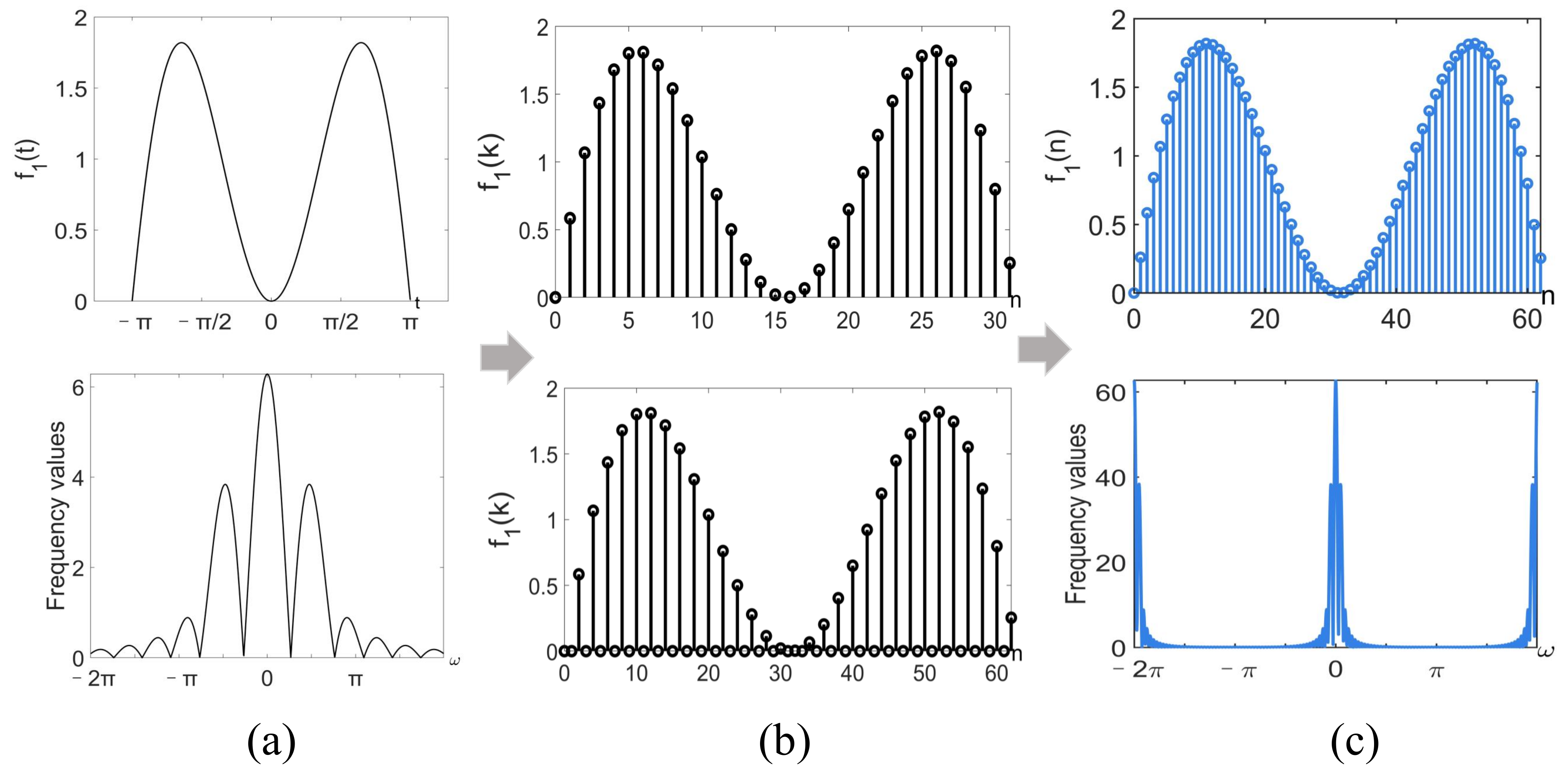
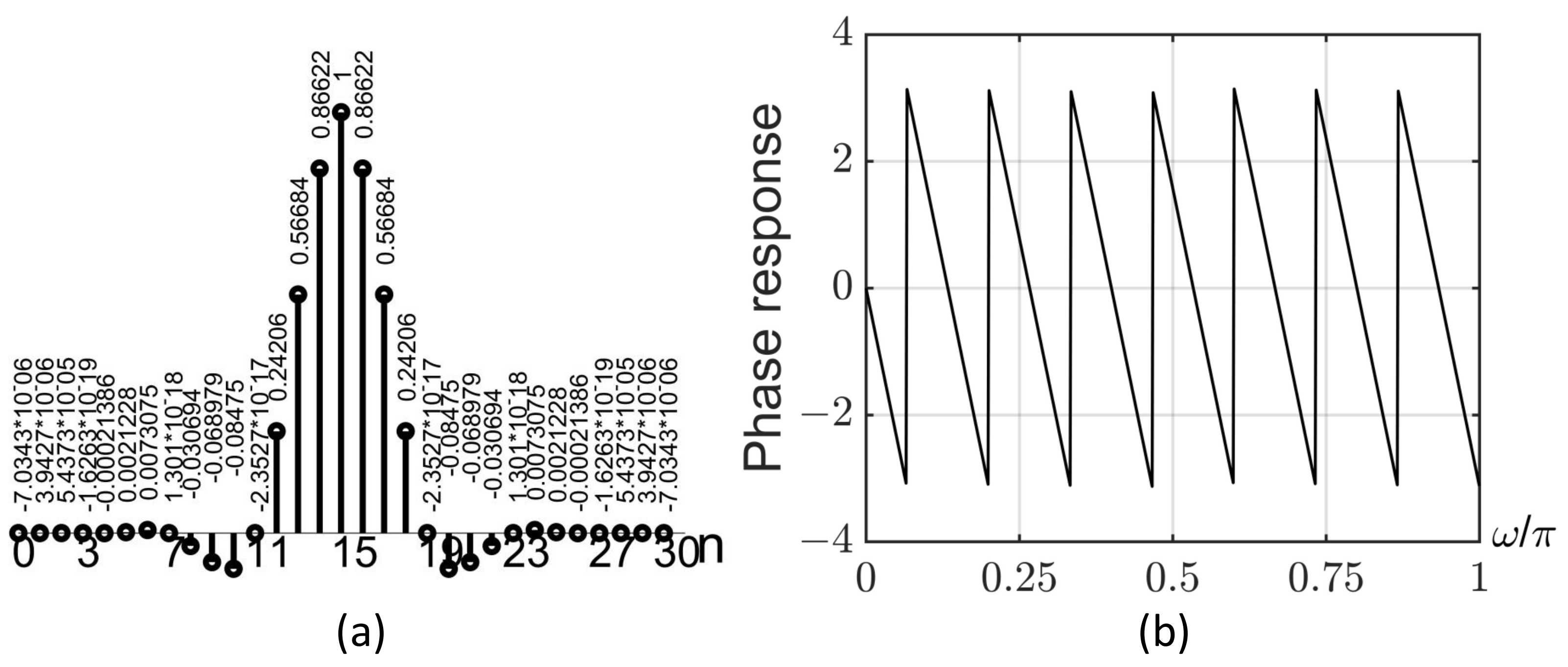
where Λ ¨ n m ( z ) is calculated by Equations (18) and (22). After the filtering of the GCP-splines, the amplitude of the filled sample is obtained from the system Λ ¨ n m ( z ) , and the amplitude of the original sample remains the same. As illustrated by the block diagram in Figure 2 and Algorithm 1, discrete GCP-spline signal filters can be achieved via two steps. An input signal is expanded to a new discrete signal by filling m 1 zero values into every two adjacent values of the original signal, and the next part is a FIR filter which shows that the filled samples are gained by the convolution. The related impulse response and phase response of the GCP-splines FIR filter with an expansion factor of four are presented in Figure 3. As shown in Figure 3b, the frequency domain reconstruction process has a linear phase as indicated; that is, the phase response is linearly related to the frequency. As mentioned earlier, linear-phase FIR filters have advantages in discrete-time reconstruction, as they can avoid phase distortion and ensure the integrity of the reconstructed signal. According to Shannon’s sampling theorem, a band-limited signal can be a perfect reconstruction by an ideal filter from a discrete signal at the Nyquist rate or higher sampling rate. However, this is impossible to achieve in practical applications, so digital filters are considered to be an approximate reconstruction of the ideal filter.
Algorithm 1 GCP-splines differential signal reconstruction
Input: Let N be the size of the original signal f ( k ) , the sampling factor m, Λ n , ϑ ( t ) with its coefficients of the average shift operator Γ ϑ = ξ 1 δ υ 1 , , ξ i δ υ i , , ξ I δ υ I , and the parameter ϑ is only used to distinguish GCP-splines of the same order n, which is the r-th order derivative of the signal p n ( r ) ( t ) ;
 1: Λ n , ϑ ( r ) = myDGCPfunc ( Γ ϑ , m ) ;
 2: f n m ˜ ( k ) = c o n v ( f ( k ) , Λ n , ϑ ( r ) ) based on Equation (25);
Output: Reconstructed differential signal data f n m ˜ ( k ) ;
 3: function myDGCPfunc ( Γ , m ) :
 4: let W = 4 : 1 / m : 4 ;
 5: for l = 1 to l e n g t h ( T )  do
 6:     Λ n , ϑ ( r ) = c o n v ( Γ ϑ , p n ( r ) ( W ( l ) ) ) based on Equation (26).
 7: end for

3.4. Differential Signal Reconstruction

Signal differentiation reconstruction involves reconstructing the derivative of a signal from its sampled values. During signal processing, differential reconstruction plays a crucial role in both theoretical and practical applications. Signal differentiation can be used to extract features of signals, such as peaks, inflection points, and transition points. These features are crucial for applications such as edge detection, noise reduction, and feature extraction. The differential signal based on the continuous GCP-splines is proposed, which is defined as
r f ˜ n ( t ) t r = k = f ( k ) r Λ n ( t k ) t r ,
and the expression of the r-order derivative of the GCP-splines in terms of the polishing splines is rewritten as
r Λ n ( t ) t r = Λ n ( r ) ( t ) = ξ 1 δ υ 1 + + ξ i δ υ i + + ξ I δ υ I p n ( r ) ( t ) ,
where Λ n ( r ) ( t ) denotes the r-th order derivative of the signal Λ n ( t ) , and the derivative of the GCP-splines is converted into the convolution of the shift operator and the derivative of polishing spline. The reconstructed differential signal based on Equation (25) is easily extended for higher-order derivatives, and it shows that the differential signal is achieved by convolution with the appropriate finite-difference operator. Therefore, the differentiation is straightforward to extend for the higher dimensions, with the reduction in the order of GCP-splines, which allows us to map these results back to the initial discrete signal space.

4. Simulated Experiments

In this section, numerical experiments on discrete signal reconstruction are presented, utilizing GCP-spline filters ( Λ 3 , i ( t ) represent the GCPF). The performance of these filters is compared with that of the cubic cardinal B-splines filters (BF) [7] and linear spline filters (LF) [7], and square and cubic polishing spline filters ( p 2 ( t ) and p 3 ( t ) ), PF [43,47]. In addition, the coefficients of the cubic cardinal B-splines interpolation filter are calculated by chasing method [7]. Assuming that the input discrete signal is derived from a known function, and the reconstructed smooth signal is obtained from the discrete-based GCP-splines signal representation based on Equation (23). As mentioned previously, the input discrete signal is derived from a known function f ( t ) . The continuous function is first processed by discretizing data, and is the interval between adjacent data (sampling step and the sample frequency f s = 1 / Hz). First, the original discrete data are preprocessed, i.e., the first and last samples are processed three times to determine the effect of sample reconstruction at both ends of the samples [44]. After the above operation using different filters, the reconstruction and differential signals are obtained from the input discrete signals.

4.1. Analog Signal

Most natural signals originate from analog signals and are then processed by digital computers. Two test functions are randomly selected to obtain discrete signal samples for signal reconstruction, and the test functions are
f 1 ( t ) = t s i n ( t ) , t [ π , π ] . f 2 ( t ) = sin ( t ) e | t | , t [ 3 π , 3 π ] .
The reconstructing effect is mainly defined by the average approximation error, which is defined as
E r r o r = f ˜ ( k ) f ( k ) 2 N ,
where · 2 follows x 2 = j = 1 n x j 2 , and N represents the total number of samples after signal amplification. Note that the denotation of the reconstructed signal with an expansion factor m is simplified as f ˜ ( k ) , and the ideal interpolated signal from the sampling of the same test signal at different rates and is simplified as f ( k ) . The time complexity is O ( m N + m Θ N ) , and m is the sampling factor, and N and Θ , respectively, are the length of the original signal f ( k ) and the coefficients Λ ¨ n m ( z ) .
To illustrate the performance of the GCP-splines filter, the results of the numerical experiments are given as shown in Figure 4 and Figure 5 and Table 1. And Circle points in the top part of Figure 2b are respectively obtained by uniform sampling function f 1 ( t ) with the sampled steps = 0.20 . Four notations A E B F , A E L F , A E p 2 and A E p 3 , and A E Λ 3 , i ( i = 1 , 2 , 3 , 4 ) are separately corresponding to the average approximation errors of the cubic B-splines filter, linear spline filter, polishing splines filters, and GCP-splines filters.
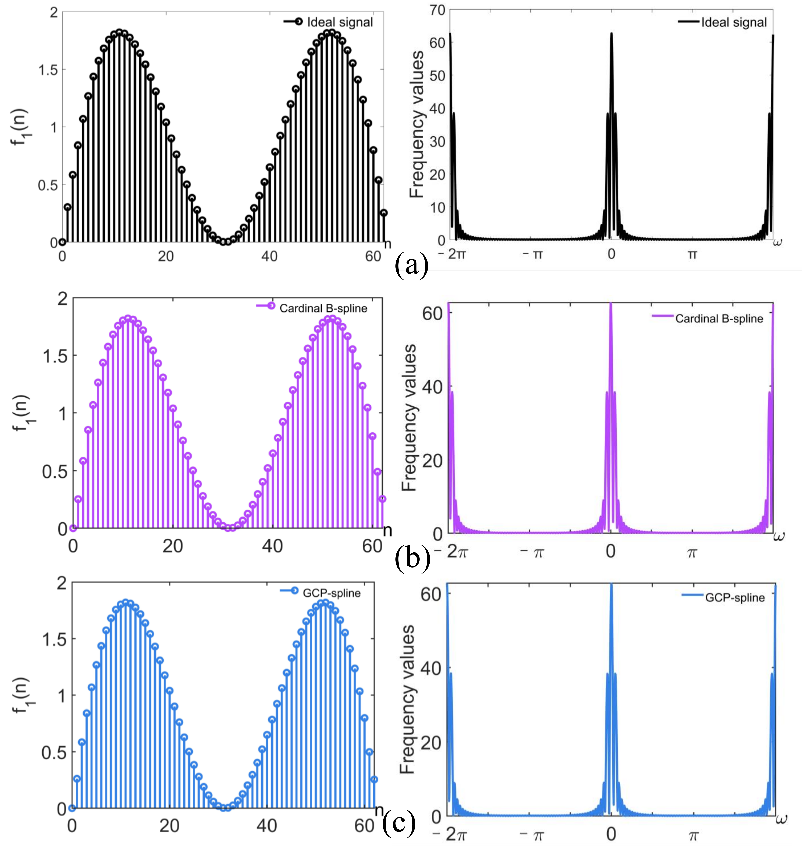
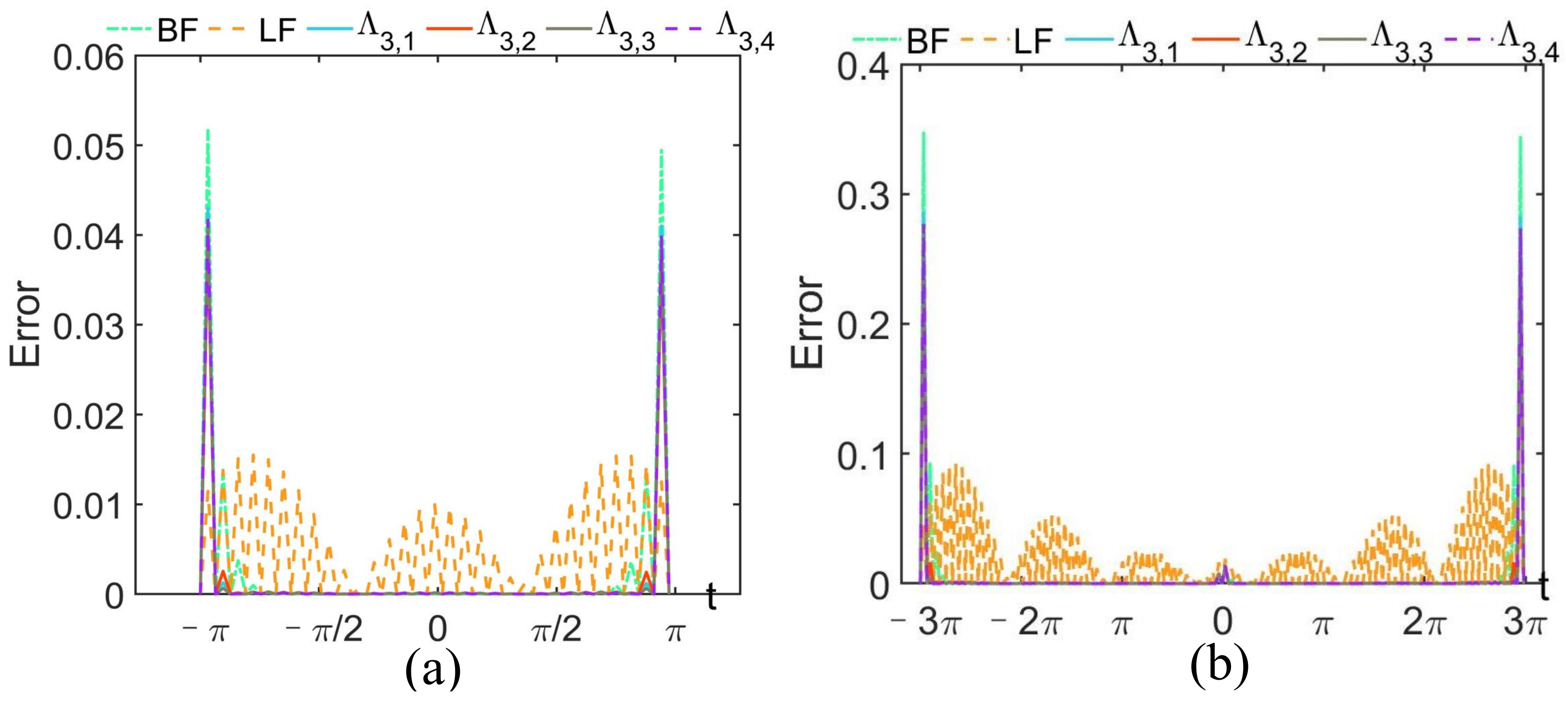
For the case in which the expanded factor of m = 2 and the sampling frequency f s = 5 Hz, the corresponding reconstruction results are presented in Figure 4. As seen from the left part of Figure 4, the reconstructed signals of the GCPF and BF are smooth and closer to the ideal interpolated signal in the discrete-time domain. Based on the right part of Figure 4, the high-frequency part of the reconstructed signal based on GCPF and BF is eliminated, although the effects of both are not easily distinguished from the visual effect. This is because the average approximation error of f 1 ( t ) is at the order of magnitude of 10 3 , which is not easy to observe directly in the graphic visualization. Moreover, the results of the average approximation error for this example using different filters are presented as follows: A E B F = 2.19 × 10 3 , and A E L F = 4.63 × 10 3 , and A E p 2 = 2.07 × 10 3 , A E p 3 = 1.62 × 10 3 , and A E Λ 3 , 2 = 1.37 × 10 3 , A E Λ 3 , 3 = 1.35 × 10 3 , and A E Λ 3 , 4 = 1.34 × 10 3 . The results of the reconstructed signals based on the GCPF have a minor approximation error compared to the cardinal B-splines, linear spline, and polishing splines, owing to high-precision GCP-splines taking into account the whole and local information. To better illustrate these differences, two error curves of the test functions f 1 ( t ) and f 2 ( t ) at each point are provided in Figure 5, providing a direct demonstration that the GCPF usually has a lower error compared with the cubic cardinal B-splines and linear spline. The linear spline has a poor effect in the frequency domain because it is a linear function with insufficient smoothness in the spatial domain.
Table 1 shows that the average approximation errors with the GCPF are generally relatively smaller than those of the cubic B-splines filter, the linear spline filter, and polishing spline filters under the same sampling step and expansion factor m. The reconstruction performance of the polishing splines filter ranks second. Although polishing splines filters are high-precision splines, they require additional pre-filtering operations during the reconstruction process, which may affect their overall efficiency. For the case of the same sampling step and different expansion factor m, the average approximation errors for each filtering algorithm decrease as the expansion factor m increases. We have a constant number of original discrete sample data, the more input data per interval sample, the worse the signal reconstruction effect. For the case of the same expansion factor m and different sampling step , the average approximation errors of each filtering algorithm tend to increase as the sampling step size becomes larger. For the same expansion factor m, the GCPF generally has a smaller approximation error than other methods as the number of sampling steps decreases. Taking function f 1 ( t ) as an example, it can be seen that the highest frequency of the function is about 6 Hz in Figure 2a. The sampling steps are 0.2, 0.1, and 0.05; that is, the corresponding sampling frequencies are 5, 10, 20. When the signal is sampled at a rate lower than or close to twice the Nyquist frequency, the GCP-splines filters reconstruct the signal with a lower reconstruction error. In addition, there are slight differences between GCP-splines, which provide multiple GCP-splines options for signal processing. This work integrates the GCP-splines into a cohesive signal processing theory through their Fourier and Z-transformations. The results indicate that compared with existing spline-based reconstruction methods, the linear phase GCP-spline filters have easy implementation and good performance in signal discrete-time reconstruction.

4.2. Differential Signal

In this section, two test functions are selected to obtain discrete signal samples for signal differentiation. The expressions of the test functions are
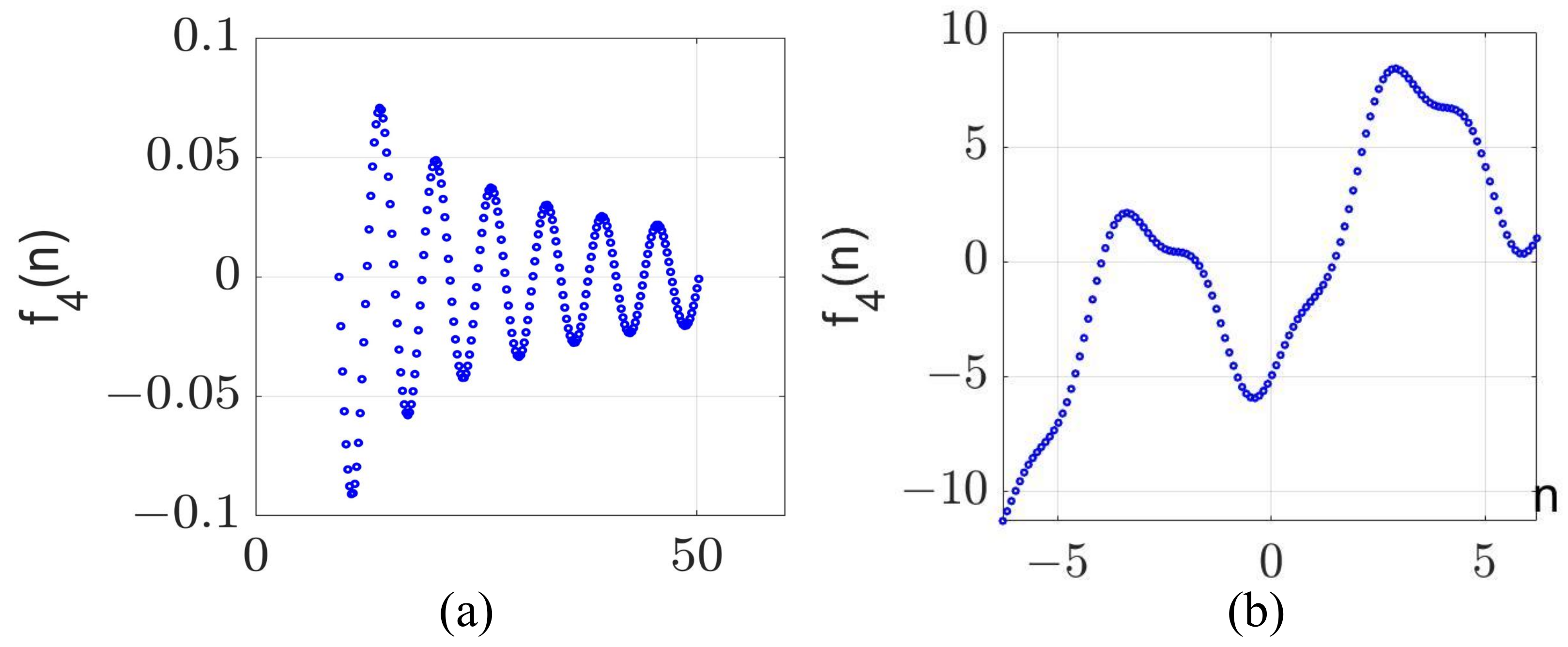
f 3 ( t ) = sin ( t ) t , t [ 3 π , 16 π ] f 4 ( t ) = t 5 cos ( t ) + sin ( 3 t ) , t [ 2 π , 2 π ] .
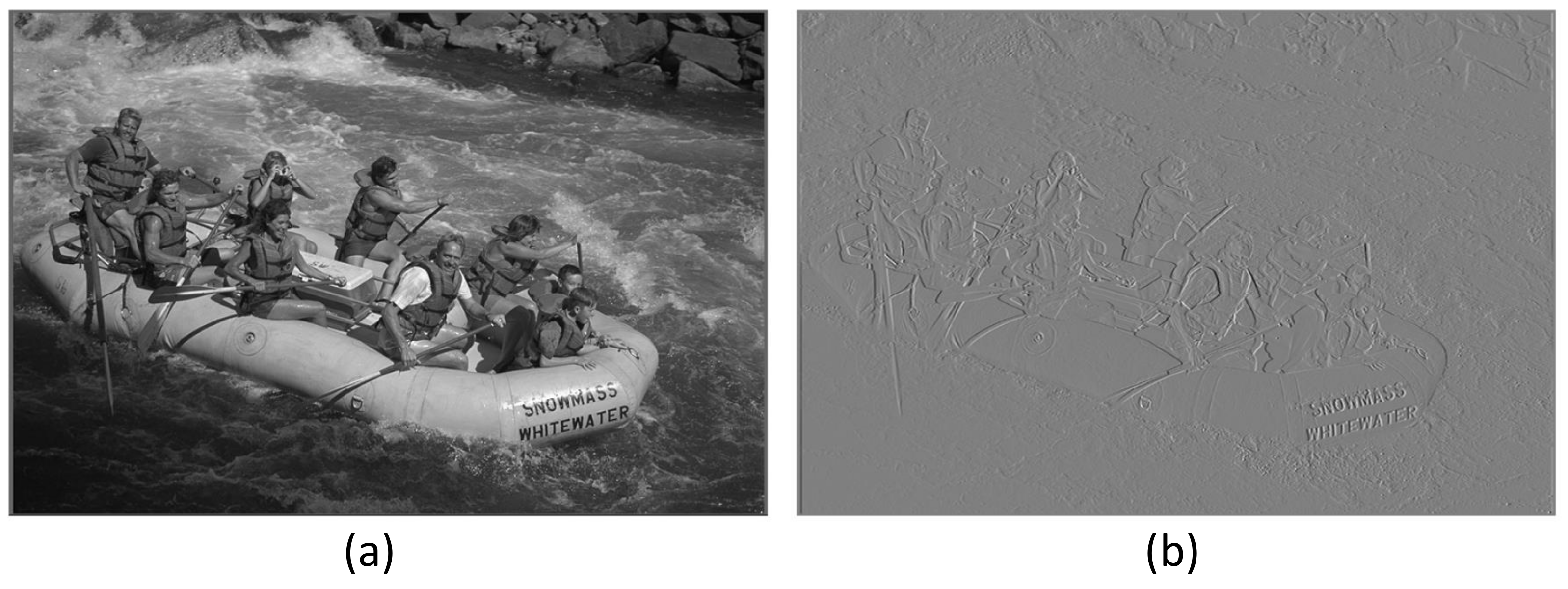
Two graphical simulation examples are provided (see Figure 6) to demonstrate the performance of differential signals using the GCP-splines. Similarly, circle points are obtained by the test functions with the sampled steps for the two examples. Taking the GCP-spline Λ 3 , 4 ( t ) function as an example, Figure 7 provides the results of first-order signal differentiation. Moreover, we present the results of the average approximation error for two examples of the differential signal based on GCP-spline and cubic B-splines, namely the error calculation between the derivative data based on splines and the derivative results of the original function. The calculation results of the first example f 3 ( t ) are A E B F = 4.83 × 10 4 and A E Λ 3 , 4 = 4.70 × 10 4 . The results of the second example f 4 ( t ) are, respectively, A E B F = 5.90 × 10 4 and A E Λ 3 , 4 = 4.68 × 10 4 . Owing to high-precision GCP-splines taking into account the whole and the local information, the results shows that the reconstructed derivative signal based on GCP-spline has a smaller average approximation error and therefore has a better reconstruction effect than B-splines. As an extension, the differential signal is extended into a two-dimensional differential image. An example of obtaining the first derivative of a grayscale image as a multidimensional signal is presented (Image sourced from [48]). As shown in Figure 8, the image is differentiated along the rows to obtain the first derivative of the image based on the GCP-spline Λ 3 , 4 ( t ) . The result is an image with wider edges, reflecting changes in the gray gradient of the image. Therefore, a feasible method for signal differentiation based on the GCP-splines is proposed, thereby paving the way for higher-order differential extensions of signals. The results show that the derivative signal based on GCP-spline has good reconstruction performance.

5. Conclusions

This paper proposes the theory of GCP-splines signal processing, including corresponding signal representations based on the GCP-splines, related Fourier transformation and Z-transformation, derivative operators of the GCP-splines, the GCP-splines filters and the differentiation signal reconstruction based on the GCP-splines. Signal reconstruction based on GCP-splines and differential signal reconstruction is achieved by changing the sampling rate signal process. The experimental results suggest that compared with cubic B-splines filters and linear spline filters, the GCP-splines filters for the reconstruction signals have better performance and achieve smooth approximation of complex signals. Owing to the superior performance of GCP-splines, their applications can be extended to diverse domains, such as surface reconstruction and integration with deep learning. Moreover, the local support characteristics of GCP-splines provide a foundation for the generation of spline wavelets. Therefore, we will further study the GCP-splines wavelet and use them to achieve multi-resolution analysis of signals.

Author Contributions

Conceptualization, F.S. and Z.C.; methodology, F.S. and Z.C.; validation, F.S. and Z.C.; formal analysis, F.S.; investigation, F.S. and Z.C.; resources, F.S.; data curation, F.S.; writing—original draft preparation, F.S.; writing—review and editing, F.S.; visualization, F.S.; supervision, Z.C.; project administration, Z.C.; funding acquisition, F.S. All authors have read and agreed to the published version of the manuscript.

Funding

This work was supported in part by the Science and Technology Development Fund of Macau under Grant 0159/2024/AMJ, in part by Guangzhou Development District International Cooperation Project (Grant No. 2023GH01).

Data Availability Statement

Data Availability Statement: The dataset used in our manuscript can be obtained at https://r0k.us/graphics/kodak/ and https://github.com/MohamedBakrAli/Kodak-Lossless-True-Color-Image-Suite (accessed on 11 March 2025).

Acknowledgments

The authors thank Dujuan Zhou and Juanjuan Chen for their careful review and advice.

Conflicts of Interest

The authors declare no conflicts of interest.

References

  1. Zhou, D.; Yuan, Z.; Cai, Z.; Zhu, D.; Shen, X. A New Local Optimal Spline Wavelet for Image Edge Detection. Mathematics 2025, 13, 42. [Google Scholar] [CrossRef]
  2. Qarariyah, A.; Yang, T.; Deng, F. A Solution-Structure B-Spline-Based Framework for Hybrid Boundary Problems on Implicit Domains. Mathematics 2024, 12, 3973. [Google Scholar] [CrossRef]
  3. Lodhi, R.K.; Darweesh, M.S.; Aydi, A.; Kolsi, L.; Sharma, A.; Ramesh, K. A Sixth-Order Cubic B-splines Approach for Solving Linear Boundary Value Problems: An In-Depth Analysis and Comparative Study. Mathematics 2024, 12, 3274. [Google Scholar] [CrossRef]
  4. Ma, X.; Shen, W. Generalized de Boor–Cox Formulas and Pyramids for Multi-Degree Spline Basis Functions. Mathematics 2023, 11, 367. [Google Scholar] [CrossRef]
  5. Zhang, B.; Zheng, H. A Variant Cubic Exponential B-splines Scheme with Shape Control. Mathematics 2021, 9, 3116. [Google Scholar] [CrossRef]
  6. Laome, L.; Budiantara, I.N.; Ratnasari, V. Estimation Curve of Mixed Spline Truncated and Fourier Series Estimator for Geographically Weighted Nonparametric Regression. Mathematics 2023, 11, 152. [Google Scholar] [CrossRef]
  7. Hsieh, S.; Andrews, H. Cubic splines for image interpolation and digital filtering. IEEE Trans. Acoust. Speech Signal Process. 1978, 26, 508–517. [Google Scholar] [CrossRef]
  8. Bohra, P.; Unser, M. Continuous-Domain Signal Reconstruction Using Lp-Norm Regularization. IEEE Trans. Signal Process. 2020, 68, 4543–4554. [Google Scholar] [CrossRef]
  9. Chen, J.; Cai, Z. A new class of explicit interpolatory splines and related measurement estimation. IEEE Trans. Signal Process. 2020, 68, 2799–2813. [Google Scholar] [CrossRef]
  10. Haro, B.B.; Vetterli, M. Sampling continuous-time sparse signals: A frequency-domain perspective. IEEE Trans. Signal Process. 2018, 66, 1410–1424. [Google Scholar] [CrossRef]
  11. Vlašić, T.; Seršić, D. Sampling and Reconstruction of Sparse Signals in Shift-Invariant Spaces: Generalized Shannon’s Theorem Meets Compressive Sensing. IEEE Trans. Signal Process. 2022, 70, 438–451. [Google Scholar] [CrossRef]
  12. Unser, M.; Aldroubi, A.; Eden, M.; Fellow, L. B-splines signal processing: Part I—Theory. IEEE Trans. Signal Process. 1993, 41, 821–833. [Google Scholar] [CrossRef]
  13. Zou, Q.; Zhu, L.; Wu, J.; Yang, Z. SplineGen: Approximating unorganized points through generative AI. Comput.-Aided Des. 2025, 178, 103809. [Google Scholar] [CrossRef]
  14. Huang, S. Implicit Uniform Rational Spline Reconstruction Method With Regularization Term. IEEE Access 2024, 12, 99012–99021. [Google Scholar] [CrossRef]
  15. Pang, D.; Ferrari, L.; Sankar, P. B-splines FIR filters. Circuits Syst. Signal Process. 1994, 13, 31–64. [Google Scholar] [CrossRef]
  16. Hosseini, M.; Plataniotis, K. Derivative kernels: Numerics and applications. IEEE Trans. Image Process. 2017, 26, 4596–4611. [Google Scholar] [CrossRef]
  17. Schoenberg, I.J. Spline functions and the problem of graduation. Proc. Nat. Acad. Sci. USA 1964, 52, 947–950. [Google Scholar] [CrossRef]
  18. Unser, M. Cardinal exponential splines: Part II—Think analog, act digital. IEEE Trans. Signal Process. 2005, 53, 1439–1449. [Google Scholar] [CrossRef]
  19. Unser, M.; Blu, T. Cardinal exponential splines: Part I—Theory and filtering algorithms. IEEE Trans. Signal Process. 2005, 53, 1425–1438. [Google Scholar] [CrossRef]
  20. Unser, M. B-splines signal processing: Part II—Efficient design and applications. IEEE Trans. Signal Process. 1993, 41, 834–848. [Google Scholar] [CrossRef]
  21. Bai, Y. On the Comparison of Trilinear, Cubic Spline, and Fuzzy Interpolation Methods in the High-Accuracy Measurements. IEEE Trans. Fuzzy Syst. 2010, 18, 1016–1022. [Google Scholar] [CrossRef]
  22. Lee, S.; Wolberg, G.; Shin, S.Y. Scattered data interpolation with multilevel B-splines. IEEE Trans. Vis. Comput. Graph. 1997, 3, 228–244. [Google Scholar] [CrossRef]
  23. Lü, Y.; Wang, G.; Yang, X. Uniform hyperbolic polynomial B-splines curves. Comput. Aided Geom. Des. 2002, 19, 379–393. [Google Scholar] [CrossRef]
  24. Qi, D.; Liang, Z. On the polish method by many-knot spline function (I). Numer. Math. J. Chin. Univ. 1979, 2, 196–209. [Google Scholar]
  25. Unser, M. Splines: A perfect fit for signal and image processing. IEEE Signal Process. Mag. 2002, 16, 22–38. [Google Scholar] [CrossRef]
  26. Ding, Q.; Wong, P.J.Y. Quintic non-polynomial spline for time-fractional nonlinear Schrdinger equation. Adv. Differ. Equ. 2020, 2020, 577. [Google Scholar] [CrossRef]
  27. Marinakis, V.; Fokas, A.S.; Kastis, G.A.; Protonotarios, N.E. Chebyshev Interpolation Using Almost Equally Spaced Points and Applications in Emission Tomography. Mathematics 2023, 11, 4757. [Google Scholar] [CrossRef]
  28. Blu, T.; Unser, M. Wavelets, fractals, and radial basis functions. IEEE Trans. Signal Process. 2002, 50, 543–553. [Google Scholar] [CrossRef]
  29. Chen, W.; Chen, T.; Wang, W. Hyperbolic polynomial B-splines with shape parameter. In Proceedings of the 2010 International Conference on Computer Application and System Modeling (ICCASM 2010), Taiyuan, China, 22–24 October 2010; pp. V10-441–V10-444. [Google Scholar] [CrossRef]
  30. Bruni, V.; Campagna, R.; Vitulano, D. Multicomponent signals interference detection exploiting HP-splines frequency parameter. Appl. Numer. Math. 2025, 209, 20–37. [Google Scholar] [CrossRef]
  31. Zhu, Y.; Han, X. C2 interpolation T-splines. Comput. Methods Appl. Mech. Eng. 2020, 362, 112835.1–112835.22. [Google Scholar] [CrossRef]
  32. Xie, J.; Xu, L.; Sun, M.; Xie, C.; Zhang, J. Quadratic Non-uniform Hyperbolic B-spline Curves. In Proceedings of the 2012 International Conference on Computer Science and Electronics Engineering, Hangzhou, China, 23–25 March 2012; pp. 508–511. [Google Scholar] [CrossRef]
  33. Vivas-Cortez, M.; Yousif, M.A.; Mohammed, P.O.; Lupas, A.A.; Ibrahim, I.S.; Chorfi, N. Hyperbolic Non-Polynomial Spline Approach for Time-Fractional Coupled KdV Equations: A Computational Investigation. Symmetry 2024, 16, 1610. [Google Scholar] [CrossRef]
  34. Munoz, A.; Blu, T.; Unser, M. Least-squares image resizing using finite differences. IEEE Trans. Image Process. Soc. 2001, 10, 1365–1378. [Google Scholar] [CrossRef] [PubMed]
  35. Fahmy, O.M.; Fahmy, M.F.; Fahmy, G.F. E-spline based image interpolators. In Proceedings of the 2014 IEEE International Symposium on Signal Processing and Information Technology (ISSPIT), Noida, India, 15–17 December 2014; pp. 61–66. [Google Scholar] [CrossRef]
  36. Schmitter, D.; Delgado-Gonzalo, R.; Unser, M. A family of smooth and interpolatory basis functions for parametric curve and surface representation. Appl. Math. Comput. 2016, 272 Pt 1, 53–63. [Google Scholar] [CrossRef]
  37. Alexandru, R.; Dragotti, P.L. Reconstructing classes of non-bandlimited signals from time encoded information. IEEE Trans. Signal Process. 2020, 68, 747–763. [Google Scholar] [CrossRef]
  38. Debarre, T.; Aziznejad, S.; Unser, M. Hybrid-spline dictionaries for continuous-domain inverse problems. IEEE Trans. Signal Process. 2019, 67, 5824–5836. [Google Scholar] [CrossRef]
  39. Nguyen, H.Q.; Bostan, E.; Unser, M. Learning convex regularizers for optimal bayesian denoising. IEEE Trans. Signal Process. 2017, 66, 1093–1105. [Google Scholar] [CrossRef]
  40. Debarre, T.; Fageot, J.; Gupta, H.; Unser, M. B-Spline-Based Exact Discretization of Continuous-Domain Inverse Problems with Generalized TV Regularization. IEEE Trans. Inf. Theory 2019, 65, 4457–4470. [Google Scholar] [CrossRef]
  41. Dadi, L.; Aziznejad, S.; Unser, M. Generating Sparse Stochastic Processes Using Matched Splines. IEEE Trans. Signal Process. 2020, 68, 4397–4406. [Google Scholar] [CrossRef]
  42. Qi, D. On the many-knot cardinal δ-spline interpolation. Acta Sci. Nat. Univ. Jilinensis 1975, 3, 70–81. [Google Scholar]
  43. Qi, D.; Tian, Z.; Zhang, Y.; Feng, J. Numerical polishing method for curve fitting. Acta Math. Sin. 1975, 18, 173–184. [Google Scholar]
  44. Chen, J.; Cai, Z. Cardinal MK-spline signal processing: Spatial interpolation and frequency domain filtering. Inf. Sci. 2019, 495, 116–135. [Google Scholar] [CrossRef]
  45. Lan, T.; Cai, Z.; Ye, B. A Novel Spline Algorithm Applied to COVID-19 Computed Tomography Image Reconstruction. IEEE Trans. Ind. Inform. 2022, 18, 7804–7813. [Google Scholar] [CrossRef]
  46. Cai, Z.; Lan, T.; Zheng, C. Hierarchical MK splines: Algorithm and applications to data fitting. IEEE Trans. Multimed. 2017, 19, 921–934. [Google Scholar] [CrossRef]
  47. Sun, F.; Cai, Z. Cubic Polishing Spline-Based Algorithms for Industrial Image Processing. IEEE Trans. Ind. Inform. 2024, 20, 314–326. [Google Scholar] [CrossRef]
  48. Sun, F.; Cai, Z. A Family of Generalized Cardinal Polishing Splines. IEEE Trans. Image Process. 2023, 33, 1952–1964. [Google Scholar] [CrossRef]
  49. Hong, S.H.; Wang, L.; Truong, T.K.; Lin, T.C.; Wang, L.J. Novel approaches to the parametric cubic-spline interpolation. IEEE Trans. Image Process. 2012, 22, 1233–1241. [Google Scholar] [CrossRef]
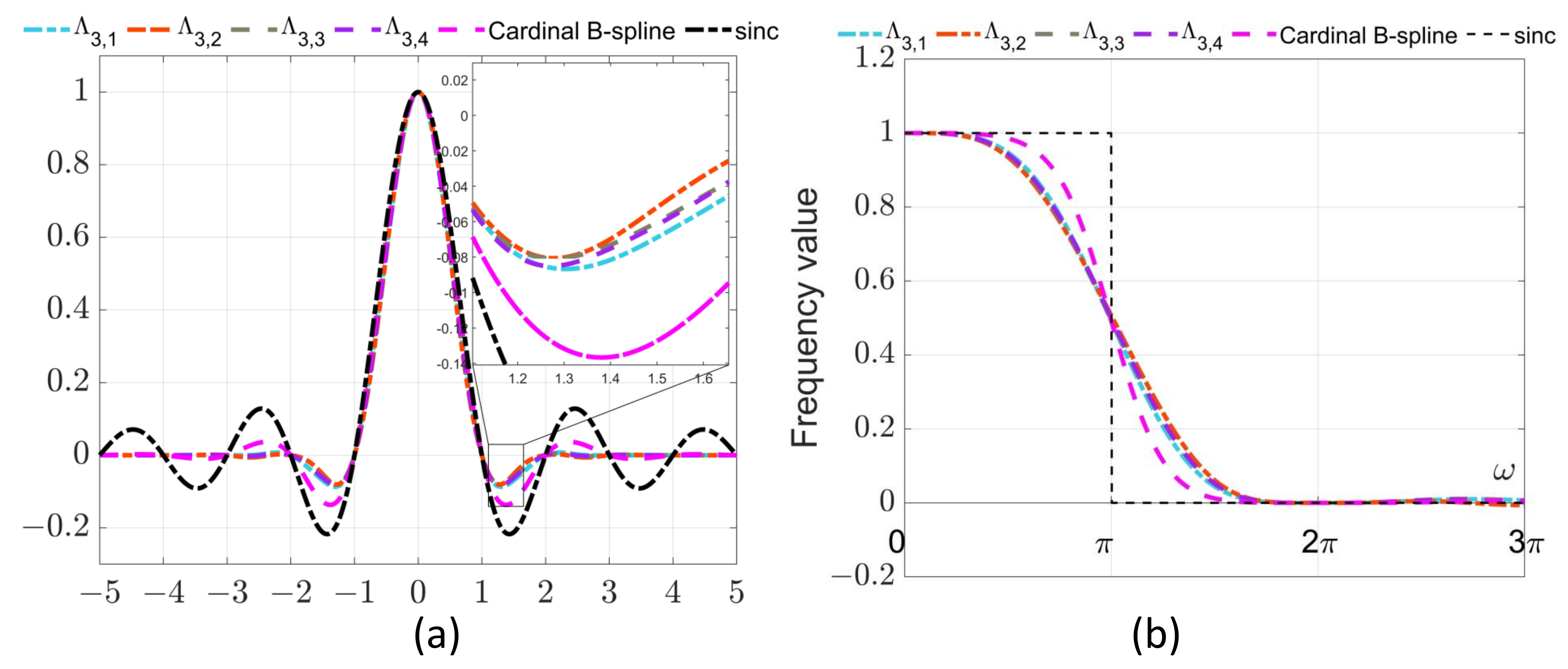
Figure 1. The GCP-splines in the frequency domain and the time domain. (a) The GCP-splines and cardinal B-splines and sinc basis functions in the time domain. (b) The GCP-splines and cardinal B-splines in the frequency domain.
Mathematics 13 00983 g001
Figure 2. Block diagram representation of the GCP-spline FIR filter procedure with expanded factor for signal processing. Sampling and filling procedures of test function f 1 ( t ) = t sin ( t ) . (a) Time and frequency domain graphs of test function f 1 ( t ) = t sin ( t ) . (b) The top part depicts sampled discrete signals with sampling step = 0.20 in the time domain; that is, the sampling frequency is 5 Hz. The bottom part depicts the samples of the expanded discrete signals with the expansion factor m = 2 . (c) Signal reconstructed using GCP-spline and the corresponding frequency domain response.
Mathematics 13 00983 g002
Figure 3. Discrete GCP-spline impulse response. (a) Discrete GCP-spline with expansion factor of four Λ 3 , 1 4 ( n 15 ) . (b) Phase response of discrete GCP-spline frequency response Λ 3 , 1 ( n ) .
Mathematics 13 00983 g003
Figure 4. Comparison of the reconstructed results of f 1 ( t ) when we have an expanded factor m = 2 and sample step = 0.20 , i.e., the sample frequency is 5 Hz. (a) The left part is the ideal signal reconstruction in the time domain, and the right part shows that of the frequency domain. (b) The signal reconstruction using the cardinal B-splines in time domain and frequency domain. (c) The signal reconstruction using the GCP-spline filter Λ 3 , 1 ( t ) in time domain and frequency domain.
Mathematics 13 00983 g004
Figure 5. Comparison of the errors corresponding to each time unit point of the two reconstructed examples when the sample step = 0.20 and the expanded factor m = 2 . (a) Error comparison of the test function f 1 ( t ) in each time unit point. (b) Error comparison of the test function f 2 ( t ) in each time unit point. The horizontal coordinate represents the each time unit point, and the vertical coordinate indicates the reconstruction average error.
Mathematics 13 00983 g005
Figure 6. (a) In the first example, the original data of f 3 ( n ) are sampled by a sampling step of = 0.2 , and the data points are taken at regular intervals of 0.2 units. (b) The second example is sampled original data of f 4 ( n ) with sampling step = 0.1 .
Mathematics 13 00983 g006
Figure 7. (a) First derivative of discrete sampling data f 3 ( n ) based on the GCP-spline Λ 3 , 4 ( t ) . (b) First derivative of discrete sampling data f 4 ( n ) based on the GCP-spline Λ 3 , 4 ( t ) .
Mathematics 13 00983 g007
Figure 8. (a) Original gray image [48] of size 768 × 512 for first derivative. (b) First differential results of the image based on the GCP-spline Λ 3 , 4 ( t ) .
Mathematics 13 00983 g008
Table 1. Error analysis of signal reconstruction using various expansion factors m and sampling steps e l l .
Sample Step and Expanded Factor  m = 2
FunctionsFilters = 0 . 2 = 0 . 1 = 0 . 05
f 1 ( t ) BF 2.19 × 10 3 5.44 × 10 4 1.36 × 10 4
LF 4.63 × 10 3 1.17 × 10 3 2.93 × 10 4
p 2 ( t ) 2.07 × 10 3 4.93 × 10 4 1.22 × 10 4
p 3 ( t ) 1.62 × 10 3 3.91 × 10 4 9.90 × 10 5
Λ 3 , 1 ( t ) 1.41 × 10 3 3.47 × 10 4 9.45 × 10 5
Λ 3 , 2 ( t ) 1.37 × 10 3 3.42 × 10 4 9.99 × 10 5
Λ 3 , 3 ( t ) 1.35 × 10 3 3.26 × 10 4 8.56 × 10 5
Λ 3 , 4 ( t ) 1 . 34 × 10 3 3 . 23 × 10 4 8 . 29 × 10 5
f 2 ( t ) BF 5.13 × 10 3 1.26 × 10 3 3.12 × 10 4
LF 1.73 × 10 2 4.34 × 10 3 1.09 × 10 3
p 2 ( t ) 4.87 × 10 3 1.15 × 10 3 2.80 × 10 4
p 3 ( t ) 3.82 × 10 3 9.16 × 10 4 2.34 × 10 4
Λ 3 , 1 ( t ) 3.36 × 10 3 8.50 × 10 4 2.56 × 10 4
Λ 3 , 2 ( t ) 3.31 × 10 3 8.73 × 10 4 3.05 × 10 4
Λ 3 , 3 ( t ) 3.20 × 10 3 7.86 × 10 4 2.20 × 10 4
Λ 3 , 4 ( t ) 3 . 18 × 10 3 7 . 69 × 10 4 2 . 03 × 10 4
Sample Step and Expanded Factor m = 4
FunctionsFilters = 0 . 2 = 0 . 1 = 0 . 05
f 1 ( t ) BF 2.76 × 10 3 6.82 × 10 4 1.70 × 10 4
LF 5.84 × 10 3 1.46 × 10 3 3.67 × 10 4
p 2 ( t ) 2.31 × 10 3 5.27 × 10 4 1.27 × 10 4
p 3 ( t ) 1.99 × 10 3 4.81 × 10 4 1.21 × 10 4
Λ 3 , 1 ( t ) 1.86 × 10 3 4.57 × 10 4 1.24 × 10 4
Λ 3 , 2 ( t ) 1.82 × 10 3 4.53 × 10 4 1.27 × 10 4
Λ 3 , 3 ( t ) 1 . 80 × 10 3 4 . 39 × 10 4 1.14 × 10 4
Λ 3 , 4 ( t ) 1.82 × 10 3 4.41 × 10 4 1 . 13 × 10 4
f 2 ( t ) BF 6.43 × 10 3 1.58 × 10 3 3.91 × 10 4
LF 2.17 × 10 2 5.44 × 10 3 1.36 × 10 3
p 2 ( t ) 5.71 × 10 3 1.27 × 10 3 2.96 × 10 4
p 3 ( t ) 4.67 × 10 3 1.12 × 10 3 2.85 × 10 4
Λ 3 , 1 ( t ) 4.39 × 10 3 1.11 × 10 3 3.36 × 10 4
Λ 3 , 2 ( t ) 4.38 × 10 3 1.15 × 10 3 3.69 × 10 4
Λ 3 , 3 ( t ) 4 . 27 × 10 3 1.06 × 10 3 2.85 × 10 4
Λ 3 , 4 ( t ) 4.29 × 10 3 1 . 05 × 10 3 2 . 78 × 10 4
The bold font indicates optimal results.
Disclaimer/Publisher’s Note: The statements, opinions and data contained in all publications are solely those of the individual author(s) and contributor(s) and not of MDPI and/or the editor(s). MDPI and/or the editor(s) disclaim responsibility for any injury to people or property resulting from any ideas, methods, instructions or products referred to in the content.