Article

Low-Complexity Relay Selection for Full-Duplex Random Relay Networks

1
SK Telecom Co., Ltd., Seoul 04539, Republic of Korea
2
School of Electrical Engineering, Kookmin University, Seoul 02707, Republic of Korea
*
Author to whom correspondence should be addressed.
Mathematics 2025, 13(6), 971; https://doi.org/10.3390/math13060971
Submission received: 27 February 2025 / Revised: 10 March 2025 / Accepted: 12 March 2025 / Published: 14 March 2025
(This article belongs to the Special Issue Computational Methods in Wireless Communication)

Abstract

:
Full-duplex relay networks have been studied to enhance network performance under the assumption that the number and positions of relay nodes are fixed. To account for the practical randomness in the number and locations of relays, this paper investigates full-duplex random relay networks (FDRRNs) where all nodes are randomly distributed following a Poisson point process (PPP) model. In addition, we propose a low-complexity relay selection algorithm that constructs the candidate relay set while considering the selection diversity gain. Our simulation results demonstrate that, rather than simply increasing the number of candidate relay nodes, selecting an appropriate candidate relay set can achieve significant performance enhancement without unnecessarily increasing system complexity.

1. Introduction

Full-duplex (FD) has attracted significant interest as a promising approach to improving the performance of wireless communication systems [1,2,3,4]. Unlike traditional half-duplex (HD) systems which exploit two orthogonal resources per link, FD enables simultaneous transmission and reception over the same time and frequency resources, theoretically doubling system capacity.
The fundamental restrictions preventing the FD system from becoming feasible is self-interference (SI), which occurs when the transmitted signal interferes with the receiver at the same node. Recent studies have made significant advancements in self-interference cancellation (SIC) techniques, making FD more viable by reducing residual SI to nearly the noise of the floor [5,6,7]. For instance, in ref. [5], reference signals are proposed to enhance digital SIC beyond 5G networks. Additionally, the joint SIC of both analog and digital domains, considering the noise enhancement effects, is proposed in ref. [6]. Furthermore, Ref. [7] investigates nonlinear SIC with auto-regression, integrating digital and analog cancellation techniques to enhance SI suppression.
With these advancements, studies on the performance of FD in various applications have been actively conducted [8,9,10]. Specifically, in ref. [8], the throughput of FD in cellular systems under distributed antennas considering the scheduling and power control algorithms is analyzed. In addition, in ref. [9], antenna structures for FD transmission in satellite systems are studied. More recently, integrated sensing and communication (ISAC) systems have adopted the FD technology to fully exploit the available degree of freedom in a reflection channel [10].
Among these applications, relay systems have been regarded a well suited candidate for integration with FD system [11,12]. Relay systems enhance coverage and improve communication reliability by forwarding data from a source to a destination through a relay node. However, conventional half-duplex relay (HDR) require separate time or frequency resources for transmission and reception to mitigate interference, leading to inefficient resource utilization. To overcome this limitation, integrating FD technology into a relay system allows simultaneous transmission and reception at the relay, fully leveraging the benefits of the relay. This has motivated extensive research on full-duplex relay (FDR) systems [13,14,15,16,17,18]. More specifically, relay transmission schemes for FDR using the amplify-and-forward (AF) and decode-and-forward (DF) protocols have been studied in refs. [13,14] and [15,16], respectively. Furthermore, relay selection algorithms for switching between HDR and FDR have been investigated in ref. [17,18].
Despite these advancements, in most prior studies, the number and locations of the relays remain fixed regardless of the channel variations. However, in practical networks, relay nodes are dynamically deployed, and their availability varies due to node mobility and network topology changes.
To address this issue, the performance of relay systems has been analyzed based on the Poisson point process (PPP) model, where all nodes are assumed to be randomly deployed in the network [19,20,21,22]. For instance, in ref. [19], the distance-based statistical properties of an HDR system for a target node have been studied under various channel models. Additionally, relay selection schemes aimed at ensuring system fairness and supporting cognitive relay systems have been investigated in refs. [20,21], respectively. In the latest works, relay selection algorithms for FDR systems that rely solely on location information have been explored in ref. [22]. However, no existing studies consider selection diversity for FDR systems.
Given that 6G networks are expected to widely adopt FD technology [23], it is crucial to develop relay selection strategies that can fully exploit selection diversity benefits while addressing the challenges posed by random relay deployments.
In this paper, we investigate the performance of FDRRNs. First, we analyze the outage probability of the full-duplex random relay networks (FDRRN) under optimal relay selection. Then, we propose a low-complexity relay selection algorithm that selects a relay node from a set of candidate relay nodes to minimize system overhead. Finally, we derive the lower bound of the outage probability and, based on this, propose a selection criterion leveraging spatial diversity.
The rest of this paper is organized as follows: Section 2 describes the network model and the outage probability of FDRRNs. In Section 3, we present the outage probability analysis for optimal relay selection and introduce a low-complexity selection algorithm designed to mitigate system overhead. Section 4 provides the simulation results, and our conclusions are summarized in Section 5.

2. System Model

In this section, we describe the system model of FDRRNs and provide the outage probability of FDRRNs. The notations used throughout this paper are summarized in Table A1.

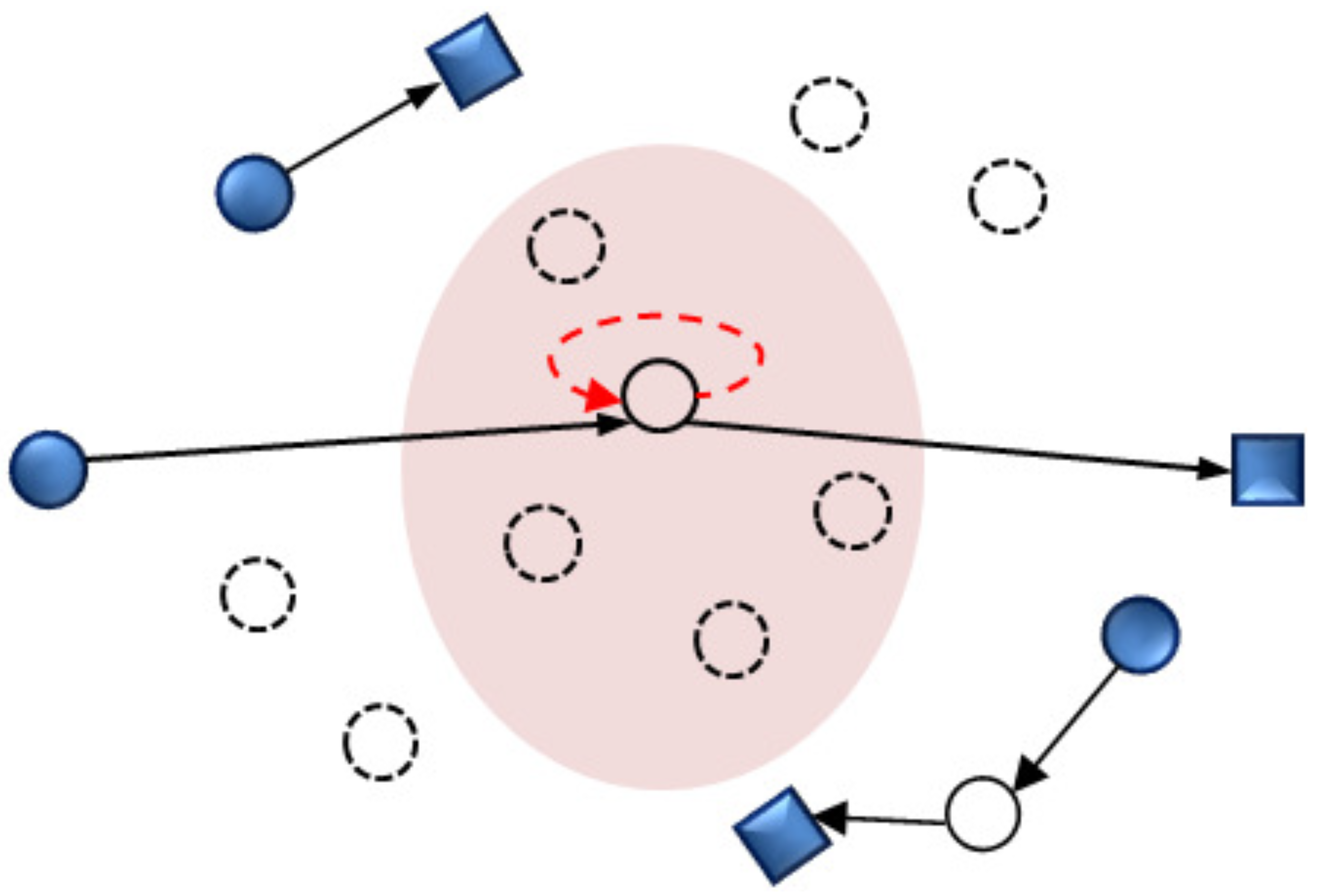
2.1. Description of FDRRN

We consider a FDRRN that consists of the transmitters, receivers, and relay nodes distributed in a 2-dimensional space according to a homogeneous PPP with spatial density λ S , λ D , and λ R , respectively, as shown in Figure 1.
The homogeneous PPP is widely recognized as a suitable model for large-scale wireless networks due to its analytical simplicity [24]. Additionally, it serves as a worst-case performance model, as all node locations are independently and identically distributed, resulting in lower interference. These characteristics make it useful for evaluating the overall network performance. Therefore, in this paper, we adopt the homogeneous PPP as an analytical model for the network. However, to account for more realistic network scenarios, alternative spatial models can be considered. The Poisson cluster point process is suitable for modeling clustered node deployment [25], while the Hard core point process is used in networks designed to minimize interference between nodes [26].
Transmitting nodes can send signals to their paired receiver nodes. However, some links between the transmitter and receiver experience outage due to unexpected fading or blockage. For those links, relay nodes can assist in maintaining reliable communication forwarding data from the source to the destination. Relay nodes are deployed separately from the transmitter and receiver nodes in the network to enhance communication between them. As a transmission mode, relay nodes utilize the DF protocol, where they first decode the received signal from the transmitter, regenerate the data, and then forward it to the receiver node. In order to establish the relay link, the FDRRN first selects a specific set of relay nodes and then chooses one relay node from this set to transmit data.
We assume that all relay nodes have a FD capability, i.e., SIC, and convey data from the source node using the DF relay protocol. In addition, relay nodes with FD transmission suffer residual SI due to the imperfect SIC. For analytical simplicity, we assume a fixed residual SI value throughout the paper [27]. Furthermore, we assume that all transmitters operate with equal transmission power, and each link is subject to Rayleigh fading and pathloss.
For the FDRRN, we assume that all nodes share the same frequency bands for communication. Hence, the transmitters generate interference to other receiving nodes. Since the distribution of the transmitter in the FDRRN follows a homogeneous PPP, the interference at the first and second relay hops also follows a PPP with spatial density λ t 1 and λ t 2 , respectively [28].

2.2. Outage Probability of the FDRRN

In this subsection, we define the signal-to-interference ratio (SIR) for the mth relay hop and then present the outage probability of the FDRRN.
When the transmitting and receiving node are located at x and y , respectively, the SIR of mth relay hop for the FDRRN can be expressed as follow:
γ m = P t x G x y L x y α I F D + Z Π m / X , Y P t x G Z Y L Z Y α , m { 1 , 2 } ,
where α is the pathloss exponent, P t x denotes the transmission power of each transmitter, and G x y and L x y represent the Rayleigh fading channel gain and the distance between the transmitter and receiver located at x and y , respectively. Furthermore, I F D denotes the residual SI after performing imperfect SIC. Note that in this paper, we consider only two-hop relay links. In other words, the first hop refers to the link between the transmitter and the relay node, while the second hop corresponds to the link between the relay node and the receiver. We also assume that both the transmission and reception antennas are isotropic, resulting in an antenna gain of 1.
Then, the outage probability of the mth relay hop for a link distance L m , i.e., P ( γ m υ ) , can be given by [22]
P γ m ( υ ) = exp I F D L m α υ P t x C α L m 2 υ 2 / α λ t m , m { 1 , 2 } ,
where υ is the target SIR threshold for the successful transmission for the link. In addition, L m is the distance of the mth relay hop and C α is a constant determined by the pathloss exponent, i.e., C α = Δ ( 2 π 2 / α ) csc ( 2 π / α ) .
In the DF relay protocol, outage occurs when either the transmitter–relay node or relay node–receiver link fails to meet the target SIR. In addition, due to the PPP, the interference affecting the transmitter–relay node and relay node–receiver links is independent. Hence, when a typical transmitter conveys its data to the receiver with the help of a relay node located at x r , the outage probability of the FDRRN can be expressed as follows:
P ( x r ) = 1 P γ 1 ( υ ) P γ 2 ( υ ) = 1 exp I F D L 1 α υ P t x C α υ 2 / α L 1 2 λ t 1 + L 2 2 λ t 2 .
According to (3), we can define the optimal relay location, which is the relay position that minimizes the outage probability for the FDRRN as follows [22]:
x o = arg min x r P ( x r ) .
On this basis, we can express (3) as a function of the distance between the optimal relay location and the relay node location.
Lemma 1.
When a source node transmits its data to the destination node via a given relay node x n located at a distance n from the optimal relay location, especially in the case of I F D 0 , the outage probability can be represented as
P ( n ) = 1 exp C α υ 2 / α λ t 1 + λ t 2 L o n 2 + 2 c o s θ λ t 2 d 2 λ t 1 d 1 L o n + λ t 1 d 1 2 + λ t 2 d 2 2 ,
where d 1 and d 2 represent the distance between the source and the optimal relay node, and the optimal relay node and the destination node, respectively.
Proof. 
Using the standard trigonometric relations, L 1 and L 2 can be rewritten as
L 1 = n 2 2 c o s θ d 1 n + d 1 2 , L 2 = n 2 + 2 c o s θ d 2 n + d 2 2 ,
where n is the distance between the relay node and the optimal relay node. In addition, θ means the angle contained between the source–optimal relay link and the relay node–optimal relay location link. By substituting L 1 and L 2 from (6) into (3) with an assumption of I F D = 0 , we can derive (5).    □
Note that we can derive the d 1 and d 2 from the optimal relay location, which was investigated in ref. [22]. For example, for the case of α = 2 , d 1 and d 2 can be represented as
d 1 = t 2 t 1 + t 2 d s d , d 2 = t 1 t 1 + t 2 d s d ,
where d s d is the distance between the source and destination. In addition, t 1 = I F D υ P t x + C α υ 2 / α λ t 1 and t 2 = C α υ 2 / α λ t 2 . Then, the outage probability for FDRRN in (5) can be given by
P ( n ) = 1 exp t 1 + t 2 L oj 2 t 1 t 2 t 1 + t 2 d s d 2 .
In (7), we can observe the relationship between the spatial densities of the interference at each relay hop and the optimal relay location. Specifically, as the interference at the first hop increases, the optimal relay location shifts closer to the source node. Conversely, as the interference in the second hop increases, the optimal relay location moves closer to the destination node. This is because the optimal relay location is adjusted to compensate for the impact of the interference and minimize outage probability. Based on this observation, we can infer the assumption that the ratio of d 1 to d 1 is proportional to that of λ t 1 to λ t 2 , i.e., λ t 1 d 1 λ t 2 d 2 . Leveraging this insight, for the remainder of this paper, let us assume λ t 1 d 1 λ t 2 d 2 to simplify the mathematical derivation and gain clearer insights.

3. Relay Selection Algorithms for the FDRRN

In this section, we investigate the relay selection algorithms that achieve selection diversity. First, we derive the outage probability of the FDRRN under the optimal relay selection, which considers all relay nodes in the network during the selection process. Then, we propose a low-complexity algorithm that selects a relay node from a set of chosen candidate relays.
Lemma 2.
For the optimal relay selection algorithm in the FDRRN, the outage probability can be expressed by
P o p t = exp π λ R C α υ 2 / α λ t 1 + λ t 2 exp C α υ 2 / α λ t 1 d 1 2 + λ t 2 d 2 2 .
Proof. 
An outage in optimal relay selection occurs only when all relays in the FDRRN fail to achieve the target SIR for a given set of relays. Based on this, the outage probability can be formulated as follows:
x n R P ( n ) ,
where Π R denotes the set of all relays in FDRRN.
Note that P ( n ) represents the outage probability for a specific relay node x n located at a distance n from the optimal relay location. Hence, the outage probability of the optimal relay selection can be represented by
P o p t = E R x n R P ( n ) ,
Then, by utilizing the probability generating function of the PPP and applying Campbell’s theorem [29], we can express (11) as
P o p t = exp 2 π λ R 0 l 1 P ( n ) d n ,
where P ( n ) is defined in (5). By performing a simple integration, we can obtain (9).    □
Note that, from Lemma 2, we can see that the outage probability of the optimal relay selection is related to the spatial density of the relay nodes, λ R . In other words, as more relay nodes become available for relay selection, the outage probability of the FDRRN improves due to the increased selection diversity.
However, in real networks, it is impractical to utilize all available relay nodes in the selection process due to computational complexity. Moreover, obtaining information such as the locations of relay nodes and channel conditions is challenging due to node mobility and channel variations As a result, selecting an appropriate set of relay nodes for the relay selection process is crucial.
In this regard, we propose a low-complexity relay selection algorithm that first selects a set of candidate relay nodes and then chooses the best relay node from the selected candidates. More specifically, the proposed algorithm first identifies J candidate relays, denoted as R , which are the nearest to the optimal relay location, ensuring that | R | = J . Under DF relay protocol, the relay node regenerates the received signal, making the link qualities of the first and second hops independent. Additionally, if either the first or second hop has poor performance, it creates a bottleneck in the communication link performance. Therefore, the max-min relay selection algorithm is optimal from a capacity perspective [30]. Following this principle, the proposed algorithm selects the best relay node among J relay nodes, as follows:
x * = arg max x r R min γ 1 , γ 2 .
An outage event occurs for J candidate relays when no relay in the candidate set meets the target SIR in the FDRRN. Hence, the outage probability of the FDRRN is given by
P J = 0 n 1 n J 1 i = 1 J P ( n ) × f N 1 , N 2 , , N J ( n 1 , n 2 , , n J ) d n 1 d n 2 d n J .
Here, N j ( j { 1 , , J } ) represents the distance from the optimal relay location to the jth nearest relay node. Additionally, the probability distribution function (PDF) of N j ( j { 1 , , J } ) , denoted as f N 1 , N 2 , , N J ( n 1 , n 2 , , n J ) , corresponds to the joint PDF of the distances to the J closest nodes to the origin due to the stationarity property of a PPP [29], and this can be expressed as follows [31]:
f N 1 , N 2 , , N J ( n 1 , n 2 , , n J ) = exp π λ R l J 2 j = 1 J l j ,
where n 1 [ 0 , ] , n j ( n j 1 , ] for j = 2 , , J .
Unfortunately, deriving a closed-form expression for the outage probability in (14) for a general J is challenging. Therefore, we analyze its lower bound under the assumption that n j is independent, as shown below.
Lemma 3.
For the relay selection among J candidate relays, the lower bound of the outage probability can be expressed as
P J = j = 1 J 1 exp C α υ 2 / α λ t 1 d 1 2 + λ t 2 d 2 2 π λ R C α υ 2 / α λ t 1 + λ t 2 + π λ R j .
Proof. 
For the case where the jth nearest relay node from the optimal relay location is selected, the outage probability can be represented as
P j = 0 P ( n ) f N j ( n j ) d n j ,
where f N j ( n j ) denotes the PDF of the distance between the optimal relay location and its jth nearest relay, N j . Owing to the stationarity property of a PPP [29], the PDF of N j is identical to that of the distance from the origin [31] to the jth nearest relay node, expressed as follows:
f N j ( n j ) = 2 ( π λ R ) j ( j 1 ) ! n j 2 j 1 e π λ R n j 2 , n j > 0 , j = 1 , 2 , .
By applying (5) and (18) into (17), P j can be obtained as
P j = 1 exp C α υ 2 / α λ t 1 d 1 2 + λ t 2 d 2 2 π λ R C α υ 2 / α λ t 1 + λ t 2 + π λ R j .
In addition, with an assumption that N j is independent for all n, we can represent (14) as
P J = j = 1 J P j .
By substituting (19) in (20), we can obtain (16).    □
From (16), we can infer the advantage of increasing the number of candidate relay nodes J. A larger set of relay nodes in the selection process can enhance the performance by leveraging increased selection diversity. However, it is also important to note that incorporating more relay nodes in the selection process introduces a trade-off between performance improvement and system overhead. More specifically, in conventional networks where the number and locations of relay nodes are fixed, channel comparison among all relay nodes is performed by obtaining their channel state information (CSI). However, in the FDRRN, as the network expands and relay nodes are randomly deployed, acquiring the CSI for all relay nodes becomes challenging. Moreover, as the number of relays increases, the amount of required information also grows, making the process more complex and resource-intensive.
Corollary 1.
As J , the ratio of the outage probability P J + 1 and P J converges to 1, i.e., lim J P J P J + 1 = 1 .
Proof. 
Using (16), we can obtain the ratio of P J + 1 and P J as follows:
P J P J + 1 = 1 exp C α υ 2 / α λ t 1 d 1 2 + λ t 2 d 2 2 π λ R C α υ 2 / α λ t 1 + λ t 2 + π λ R J + 1 .
Here, since C α , υ , λ t 1 , λ t 1 , λ t 2 , and λ R > 0 , we have π λ R C α υ 2 / α λ t 1 + λ t 2 + π λ R J + 1 < 1 . Thus, we can obtain Corollary 1.    □
Corollary 1 reveals that the relay nodes which are far away from the optimal relay location are not beneficial for performance gain. In other words, by excluding relay nodes that do not contribute to selection diversity in the candidate relay set, we can improve system overhead while maintaining proper performance. Considering this observation, we can define the spatial diversity gain as follows:
G J = P J P J + 1 .
By setting an appropriate threshold greater than 1 for the spatial diversity gain, considering the system requirements, we can determine whether to include the Jth nearest relay node in the candidate relay set.
In summary, the low-complexity relay selection algorithm follows the steps below to select a relay node:
  • Step 1: The transmitter and receiver determine the temporary number of candidate relay nodes, J t m p , that the system can accommodate for CSI feedback, considering the system resource constraints.
  • Step 2: The transmitter and receiver compute the selection diversity gain for J = J t m p , G J t m p . If G J t m p exceeds a predefined threshold τ , the current number of candidate relay nodes is adopted, i.e., J = J t m p . Otherwise, the number of candidate relay nodes is reduced by one, i.e., J t m p = J t m p 1 , and the process repeats until the selection diversity gain satisfies the threshold condition. The detailed procedure for Step 2 is outlined below:
  • Step 3: The J candidate relays are selected based on their proximity to the optimal relay location.
  • Step 4: The transmitter and receiver acquire the CSI of the selected candidate relay nodes and finalize the relay selection using the max-min relay selection Algorithm 1.
Algorithm 1 Determination of the number of candidate relay nodes
1:
Compute the selection diversity gain G J t m p
2:
while  G J t m p < τ   do
3:
      Reduce the number of candidate relay nodes: J t m p = J t m p 1
4:
      Recompute the selection diversity gain G J t m p
5:
end while
6:
Set J = J t m p
In conventional relay networks where the relay node positions are fixed, utilizing a more number of candidate relay nodes leads to a linear increase in selection diversity. In contrast, in real networks, selection diversity varies depending on the relay node locations. To account for this characteristic, the proposed algorithm determines the appropriate candidate relay nodes and their number by considering the network parameters and the corresponding diversity gain. This enables efficient relay selection in practical network environments.

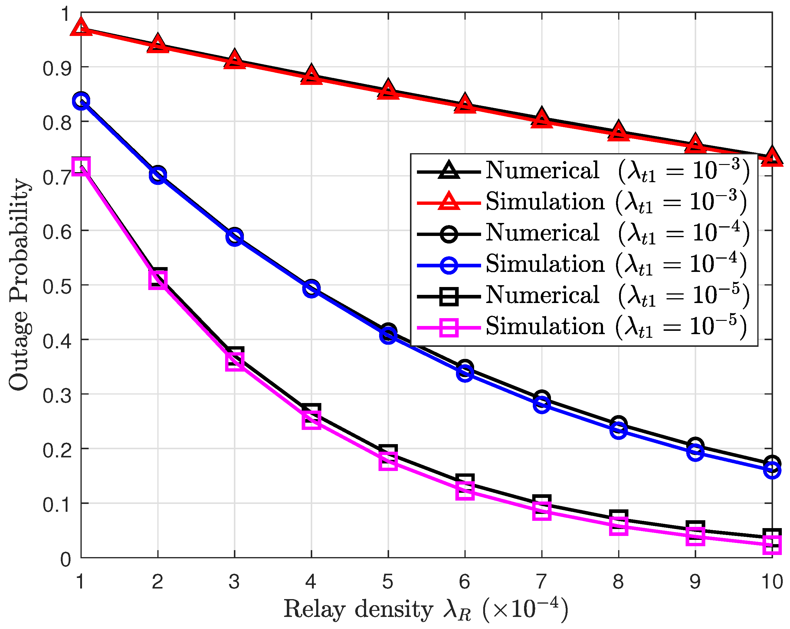
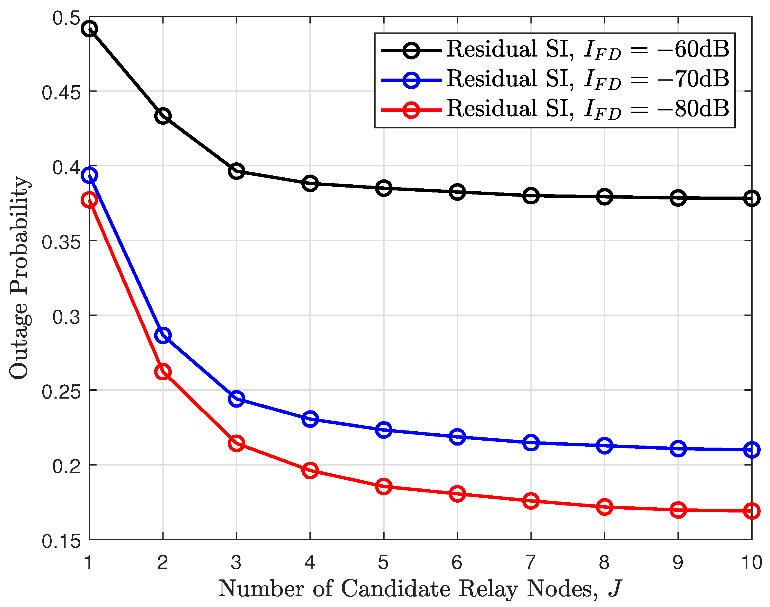
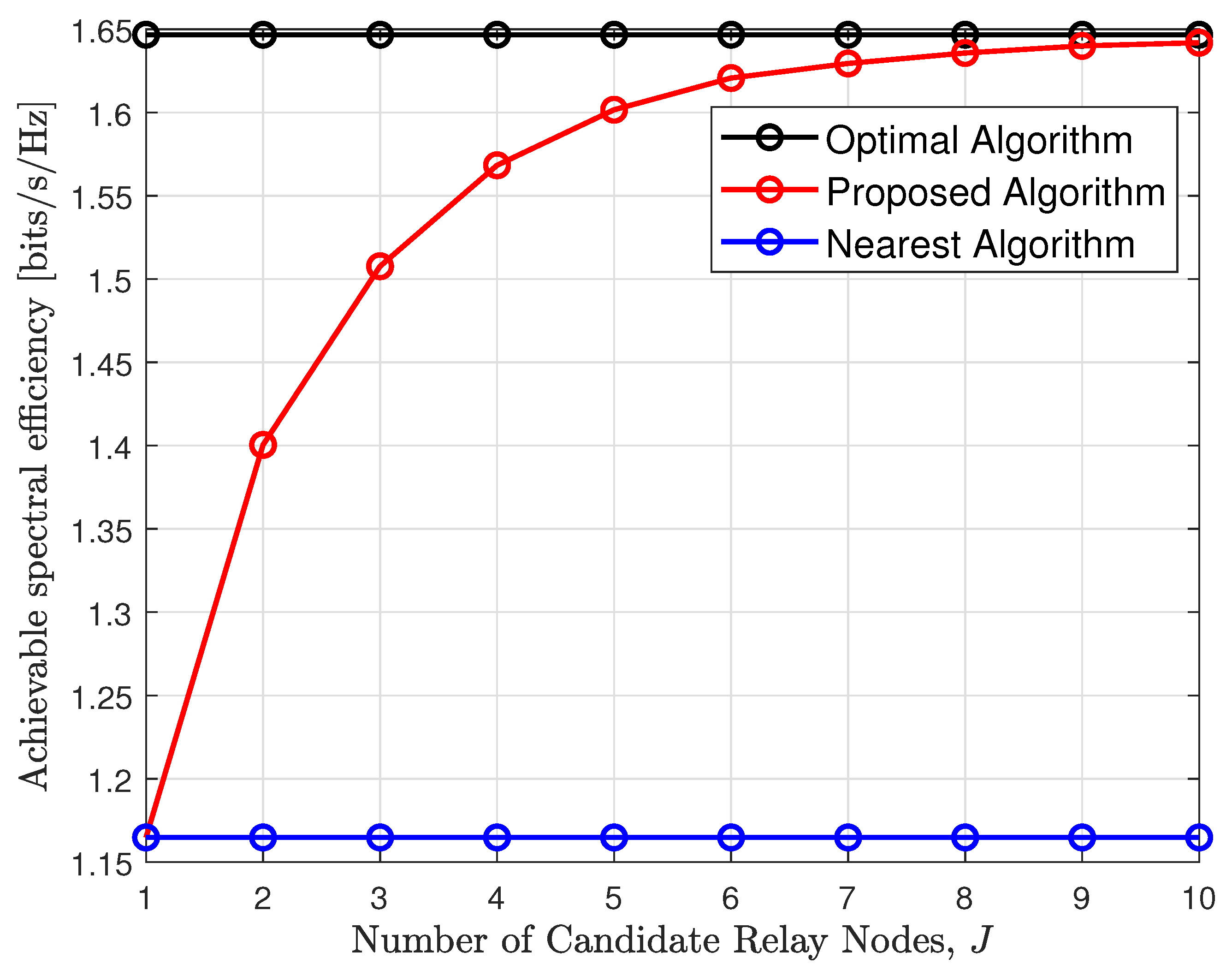
4. Simulation Results

In this section, we analyze the performance of the FDRRN by simulating the proposed relay selection algorithm across different scenarios. The simulations are conducted using the system parameters provided in Table 1, unless stated otherwise.
In the simulation, candidate relay nodes and interfering nodes are uniformly distributed within a cell of radius 300 m according to their spatial density. Additionally, all transmitting nodes use a normalized transmission power of 1. To ensure reliable FD transmission, a SIC level of approximately 110 dB is required; therefore, I F D is set to 110 dB [1].
Figure 2 illustrates the outage probability of the FDRRN under optimal relay selection for varying spatial densities of relay nodes and interference. As observed in the figure, the numerical results closely follow the trend of the simulation results, with only a negligible difference as the spatial densities of relay nodes and interference increase. These results verify the validity of λ t 1 d 1 λ t 2 d 2 , which was assumed for the derivation of Lemma 1. Furthermore, it can be observed that as the spatial density of relay nodes increases, the overall performance of the FDRRN improves. This is because a larger number of relay nodes participating in the relay selection algorithm enhances selection diversity, providing a greater opportunity to choose a relay node with better performance.
Figure 3 shows the outage probability of the low-complexity relay selection as a function of the number of candidate relay nodes under different levels of residual SI. It is evident that an increase in residual SI leads to a higher outage probability. In addition, as the number of candidate relay nodes increases, the outage probability decreases. This is due to the fact that a larger number of candidate relay nodes increases the likelihood of selecting a relay node that ensures reliable communication.
Figure 4 depicts the outage probability of FDRRN for low-complexity relay selection with different numbers of candidate relay nodes, represented by blue circles, and its lower bound, given by (16), shown as a dashed line.
We can see that the lower-bound analysis exhibits a similar trend to the simulation results with a slight variation. In addition, it can be observed that as the number of candidate relay nodes increases, the improvement in outage probability gradually diminishes. This is due to the fact that as more candidate relay nodes are included, relay nodes located farther from the optimal relay location participate in the candidate relay set, which contributes only marginally to performance improvement.
Figure 5 shows the spatial diversity gain of the FDRRN, as defined in (22), for low-complexity relay selection under different spatial densities of relay nodes. We can observe that the spatial density gain decreases at a slower rate as the spatial density of relay nodes increase. This is because, with a higher spatial density, more relay nodes are likely to be located near the optimal relay location. Additionally, the spatial diversity gain can be utilized to determine the appropriate size of the candidate relay set. For instance, if the system constrains the candidate relay set to include only nodes that achieve at least a 5% spatial diversity gain, the number of candidate relay nodes would be 7 for λ R = 1 × 10 3 .
Figure 6 shows the achievable spectral efficiency of the FDRRN according to the various relay selection algorithms. The achievable spectral efficiency is given by the product of the successful transmission probability and the spectral efficiency of the DF relay protocol [32], expressed as follows:
ς = 1 P J × min log 2 1 + γ 1 , log 2 1 + γ 2 .
It is observed that the achievable spectral efficiency of the proposed algorithm improves as relay density increases, owing to the enhanced selection diversity. In addition, the proposed algorithm performs comparably to the optimal relay selection algorithm at a certain number of candidate relay nodes. This indicates that simply increasing the number of relay nodes that do not contribute to selection diversity results in higher system complexity without meaningful performance improvement. Furthermore, the nearest algorithm proposed in ref. [22] selects only a single relay node closest to the optimal relay location, resulting in no improvement as the number of candidate relay nodes increases. However, it achieves the lowest system complexity.

5. Conclusions

This paper investigated the relay selection scheme for the FDRRN based on stochastic analysis, accounting for the random nature of practical networks. We demonstrated that simply increasing the number of candidate relay nodes does not necessarily lead to performance enhancement. Based on this observation, we proposed a low-complexity relay selection algorithm that determines the candidate relay set size by balancing performance and overall system complexity through selection diversity gain. The obtained results provide valuable insights for designing more efficient and reliable full-duplex relay networks. Furthermore, this study opens several avenues for future research on the FDRRN, including relay selection from an energy efficiency perspective and the integration of AI/ML-based algorithms.

Author Contributions

Conceptualization, J.B. and T.K.; methodology, J.B.; software, J.B.; validation, J.B. and T.K.; formal analysis, J.B.; investigation, J.B. and T.K.; visualization, J.B.; writing—original draft preparation, J.B.; writing—review and editing, T.K.; funding acquisition, T.K. All authors have read and agreed to the published version of the manuscript.

Funding

This work was supported by the Institute of Information communications Technology Planning Evaluation (IITP) grant funded by the Korean government (MSIT) (No. RS-2024-00397789, Development and Standardization of 6G Radio Transmission Standard Technology).

Data Availability Statement

The raw data supporting the conclusions of this article will be made available by the authors on request.

Conflicts of Interest

Author Jonghyun Bang was employed by the company SK Telecom Co., Ltd. The remaining authors declare that the research was conducted in the absence of any commercial or financial relationships that could be construed as a potential conflict of interest.

Appendix A

Table A1. Notations used throughout the paper.
NotationDefinition
P t x Tx. power of each node
G x y Fading gain of the link between nodes x and y
L x y Distance between nodes x and y
L m Distance of mth relay hop
I F D Residual SI
γ m SIR of mth relay hop
α Pathloss exponent
υ Target SIR of the FDRRN
Π m PPP for interfering node of mth relay hop
Π R PPP for relay nodes
λ t m Spatial density of interfering node of mth relay hop
λ R Spatial density of candidate relay nodes
P o p t The outage probability of optimal relay seleciton
P J The outage probability for a low-complexity scheme
P J The lower bound of outage probability for low-complexity scheme
x r Location of relay nodes
x o Optimal relay location
x n Relay located at a distance n from the optimal relay location

References

  1. Kim, D.; Lee, H.; Hong, D. A survey of in-band full-duplex transmission: From the perspective of PHY and MAC layers. IEEE Commun. Surv. Tutor. 2015, 17, 2017–2046. [Google Scholar] [CrossRef]
  2. Mohammadi, M.; Mobini, Z.; Galappaththige, D.; Tellambura, C. A comprehensive survey on full-duplex communication: Current solutions, future trends, and open issues. IEEE Commun. Surv. Tutor. 2023, 25, 2190–2244. [Google Scholar] [CrossRef]
  3. Kim, Y.; Moon, H.J.; Yoo, H.; Kim, B.; Wong, K.K.; Chae, C.B. A State-of-the-art Survey on Full-duplex Network Design. Proc. IEEE 2024, 112, 463–486. [Google Scholar] [CrossRef]
  4. Smida, B.; Wichman, R.; Kolodziej, K.E.; Suraweera, H.A.; Riihonen, T.; Sabharwal, A. In-Band Full-Duplex: The Physical Layer. Proc. IEEE 2024, 112, 322–462. [Google Scholar] [CrossRef]
  5. Mori, S.; Mizutani, K.; Harada, H. A digital self-interference cancellation scheme for in-band full-duplex-applied 5G system and its software-defined radio implementation. IEEE Open J. Veh. Technol. 2023, 4, 444–456. [Google Scholar] [CrossRef]
  6. Le, A.T.; Huang, X.; Ding, C.; Zhang, H.; Guo, Y.J. An In-Band Full-Duplex Prototype With Joint Self-Interference Cancellation in Antenna, Analog, and Digital Domains. IEEE Trans. Microw. Theory Tech. 2024, 4, 5540–5549. [Google Scholar]
  7. Dong, Q.; Austin, A.C.; Sowerby, K.W. Augmentation of Self-Interference Cancellation for Full-Duplex using NARX Neural Networks. IEEE Wirel. Commun. Lett. 2023, 13, 810–813. [Google Scholar] [CrossRef]
  8. Fukushima, K.; Mori, S.; Mizutani, K.; Harada, H. Throughput enhancement of dynamic full-duplex cellular system by distributing base station reception function. IEEE Open J. Veh. Technol. 2022, 4, 114–126. [Google Scholar] [CrossRef]
  9. Choi, D.; Byun, G. Circular polarization conversion using dual frequency selective surfaces for full-duplex satellite communications. IEEE Access 2024, 12, 120219–120225. [Google Scholar] [CrossRef]
  10. Cho, W.; Chang, K.; Shin, W.; Kim, Y.; Ko, Y.J. OFDM-Based In-Band Full-Duplex ISAC Systems. IEEE Wirel. Commun. Lett. 2025, 14, 365–369. [Google Scholar] [CrossRef]
  11. Liu, G.; Yu, F.R.; Ji, H.; Leung, V.C.; Li, X. In-band full-duplex relaying: A survey, research issues and challenges. IEEE Commun. Surv. Tutor. 2015, 17, 500–524. [Google Scholar] [CrossRef]
  12. Shen, H.; He, Z.; Xu, W.; Gong, S.; Zhao, C. Is full-duplex relaying more energy efficient than half-duplex relaying? IEEE Wirel. Commun. Lett. 2019, 8, 841–844. [Google Scholar] [CrossRef]
  13. Shao, Y.; Gulliver, T.A. Transceiver Optimization for Multiuser Multiple-Input Multiple-Output Full-Duplex Amplify-and-Forward Relay Downlink Communications. Telecom 2024, 5, 216–227. [Google Scholar] [CrossRef]
  14. Zhao, J.; Jiang, D.; Wei, H.; Liu, B.; Zhao, Y.; Zhang, Y.; Liu, X. Joint Hybrid Beamforming Design for Millimeter Wave Amplify-and-Forward Relay Communication Systems. Appl. Sci. 2024, 14, 3713. [Google Scholar] [CrossRef]
  15. Shim, Y.; Shin, W.; Vaezi, M. Relay power control for in-band full-duplex decode-and-forward relay networks over static and time-varying channels. IEEE Syst. J. 2021, 16, 33–40. [Google Scholar] [CrossRef]
  16. Shao, Y.; Wang, L.; Xue, Y. Distributed alamouti protocol for full-duplex decode-and-forward relaying networks. IEEE Commun. Lett. 2021, 26, 182–186. [Google Scholar] [CrossRef]
  17. Siddig, A.A.; Ibrahim, A.S.; Ismail, M.H. A low-delay hybrid half/full-duplex link selection scheme for cooperative relaying networks. IEEE Trans. Veh. Technol. 2022, 71, 11174–11188. [Google Scholar] [CrossRef]
  18. Ma, J.; Huang, C.; Li, Q. Energy efficiency of full-and half-duplex decode-and-forward relay channels. IEEE Internet Things J. 2022, 9, 9730–9748. [Google Scholar] [CrossRef]
  19. Behnad, A.; Wang, X. Distance statistics of the communication best neighbor in a Poisson field of nodes. IEEE Trans. Commun. 2015, 63, 997–1005. [Google Scholar] [CrossRef]
  20. Sadeghi, M.; Rabiei, A.M. A fair relay selection scheme for a DF cooperative network with spatially random relays. IEEE Trans. Veh. Technol. 2017, 66, 11098–11107. [Google Scholar] [CrossRef]
  21. Bang, J.; Lee, J.; Kim, S.; Hong, D. An efficient relay selection strategy for random cognitive relay networks. IEEE Trans. Wirel. Commun. 2014, 14, 1555–1566. [Google Scholar] [CrossRef]
  22. Bang, J.; Kim, T. Location-Based Relay Selection in Full-Duplex Random Relay Networks. Appl. Sci. 2024, 14, 10626. [Google Scholar] [CrossRef]
  23. Smida, B.; Sabharwal, A.; Fodor, G.; Alexandropoulos, G.C.; Suraweera, H.A.; Chae, C.B. Full-duplex wireless for 6G: Progress brings new opportunities and challenges. IEEE J. Sel. Areas Commun. 2023, 14, 2729–2750. [Google Scholar] [CrossRef]
  24. Win, M.Z.; Pinto, P.C.; Shepp, L.A. A mathematical theory of network interference and its applications. Proc. IEEE 2009, 97, 205–230. [Google Scholar] [CrossRef]
  25. Haenggi, M.; Ganti, R.K. Interference in large wireless networks. Found. Trends® Netw. 2009, 3, 127–248. [Google Scholar] [CrossRef]
  26. Chiu, S.N.; Stoyan, D.; Kendall, W.S.; Mecke, J. Stochastic Geometry and Its Applications; John Wiley & Sons: Hoboken, NJ, USA, 2013. [Google Scholar]
  27. Lee, J.; Quek, T.Q. Hybrid full-/half-duplex system analysis in heterogeneous wireless networks. IEEE Trans. Wirel. Commun. 2015, 14, 2883–2895. [Google Scholar] [CrossRef]
  28. Baccelli, F.; Blaszczyszyn, B.; Muhlethaler, P. An Aloha protocol for multihop mobile wireless networks. IEEE Trans. Inf. Theory 2006, 52, 421–436. [Google Scholar] [CrossRef]
  29. Kingman, J. Poisson Process; Oxford University Press: Oxford, UK, 1993. [Google Scholar]
  30. Luo, S.; Teh, K.C. Buffer state based relay selection for buffer-aided cooperative relaying systems. IEEE Trans. Wirel. Commun. 2015, 14, 5430–5439. [Google Scholar] [CrossRef]
  31. Moltchanov, D. Distance distributions in random networks. Ad Hoc Netw. 2012, 10, 1146–1166. [Google Scholar] [CrossRef]
  32. Ju, M.; Kim, I.M.; Kim, D.I. Joint relay selection and relay ordering for DF-based cooperative relay networks. IEEE Trans. Commun. 2012, 60, 908–915. [Google Scholar] [CrossRef]
Figure 1. Example of a FDRRN where blue circles and squares denote the transmitter and receiver nodes, respectively. Furthermore, the empty black circles with dotted lines represent relay nodes, while those with solid lines indicate the selected relay nodes. Note that the selected relay node is chosen among the set of candidate relays located within the red circle. In addition, the red dotted arrow denotes the impact of residual SI on the relay node.
Mathematics 13 00971 g001
Figure 2. Outage probability of the FDRRN with optimal relay selection as a function of the spatial density of the relay nodes, including both the numerical and simulation results when λ t 2 = 10 4 .
Mathematics 13 00971 g002
Figure 3. Outage probability of the FDRRN as a function of the candidate relay node density with different residual SI, I S I .
Mathematics 13 00971 g003
Figure 4. Outage probability of the FDRRN with low-complexity relay selection as a function of the number of candidate relay nodes, including both simulation and lower-bound results.
Mathematics 13 00971 g004
Figure 5. Spatial diversity gain of the FDRRN according to the number of candidate relay nodes with different spatial density of relay nodes.
Mathematics 13 00971 g005
Figure 6. Achievable spectral efficiency of the FDRRN as a function of the number of candidate relay nodes for various relay selection algorithms.
Mathematics 13 00971 g006
Table 1. Simulation parameters.
ParametersValues
Pathloss exponent, α 4
Target SIR threshold, υ 3
Spatial density of interference, λ 1 , λ 2 10 4
Spatial density of relay, λ R 10 3
Cell radius300 m
Distance between source and destination10 m
Residual SI, I F D −110 dB
Tx. power, P t x 1
Disclaimer/Publisher’s Note: The statements, opinions and data contained in all publications are solely those of the individual author(s) and contributor(s) and not of MDPI and/or the editor(s). MDPI and/or the editor(s) disclaim responsibility for any injury to people or property resulting from any ideas, methods, instructions or products referred to in the content.

