2. Semantic Representation of Parallel–Hierarchical Networks
Let us represent the process of information processing by parallel–hierarchical networks at the semantic level. First, it is important to note that the cerebral cortex contains a multitude of nerve cells to which afferent impulses converge (carrying excitation to the central nervous system) from various receptors—visual, auditory, thermal, muscular, and others. This indicates the existence of a complex mechanism of interactions between different cortical zones. The presence of this interaction mechanism suggests specific features of the computational organization in the cortex: topographical mapping, simultaneous (parallel) signal processing, the mosaic structure of the cortex, coarse cortical hierarchy, a spatially and temporally correlated perception mechanism, and learning capabilities [
3].
However, the main unresolved question remains: how does the interaction of nerve cells, which occurs at the moment of stimulus convergence, become structured in the cerebral cortex? At the structural level, the organization of cortical zones as interacting neural networks can be presented as shown in
Figure 1.
Here, each layer of cortical zones is represented as a neural network, illustrating a neurobiological process of hierarchically interdependent interactions between convergent–divergent structures. Furthermore, the homologous outputs of subsequent neural networks are Each output corresponding to cortical zones forms the respective input for the next cortical zone. The term “homologous outputs” implies a multiple correlation process of temporal signal coincidence at these inputs.
Neural networks are an ideal mechanism capable of stable operation in uncertain conditions [
5]. Neural networks that function based on the principle of dynamic multifunctionality incorporate interactions of convergent–divergent structures in both horizontal and vertical directions, forming a 3D architecture. In such a structure, the complexity of various convergent–divergent process schemes enables variations (genetically governed changes) in the trajectories of horizontal pathways. These pathways may also slightly adjust during the learning process.
To better understand the proposed neural network, let us draw some semantic analogies. Imagine a group of researchers jointly solving a specific scientific problem [
6]. Each has its own knowledge base related to the issue. They express their judgments of the problem and arrive at a common conclusion, creating a matrix of judgments representing the first level of discussion.
At each subsequent level of problem solving, the first intermediate result of the discussion undergoes further refinement, forming a matrix of judgments. This refinement is performed whenever all judgments at a given moment in time converge to some approximation. This occurs when, from many divergent judgments, a general judgment is formed that satisfies all researchers. The intermediate results of the discussion are refined outcomes from the previous discussion level. All of them are decorrelated from the other (current) results of the discussion.
The overall result of the discussion is a sequential process of multistage refinement of the problem being solved and consists of individual intermediate judgments [
3,
4,
5]. Therefore, the parallel–hierarchical process can be defined as the simultaneous analysis of a phenomenon (or object) by identifying hierarchies of increasingly effective representations of it.
An example of the semantic organization of this process is shown in
Figure 2, where 1N, 2N, and 3N are the first, second, and third observers identifying a certain visual pattern, and
are the results of visual scene identification.
The specific semantic content of the nodes in the formed network can be, for example, as follows: 11—there is an object on the surface of the rail head; 12—the object is located on the working face of the rail; 13—the surface of the object has depressions; 14—the object is mainly dark in color; 15—there is an influx of metal on the working edge of the rail head; 16—the handicap of the object is complicated; 17—the object is not similar to a foreign object; 18—the surface of the object is different from the surface of the rail; 19—there are dark spots near the working edge of the rail head; 21—the object on the rail looks like a defect; 22—the object is stretched along the rail; 23—the length of the object is more than 25 mm; 24—there is a micro crack on the working edge of the rail head; 25—an unusual shape; 26—it seems to be about an object of an elongated shape; 27—the depth of irregularities on the object is more than 1 mm; 31—indentations are similar to metal exfoliation; 32—coloration is similar to a defect; 33—the object has metal inhomogeneity; 41—the object on the rail refers to the defect scraping of metal on the side working circle of the head due to insufficient contact–fatigue strength of the metal, which has a ripping depth of 1 mm and a ripping length of 25 mm.
In the examined example, it is clear that the proposed semantic AI network (
Figure 2) is a semantic organization of a dynamic data structure consisting of nodes representing time-varying objects or concepts, as well as links that indicate the temporal relationship between the nodes.
Unlike known structures of semantic networks, here, it becomes clear how to represent a situation in the network as an exception to the rules. Analogous to the known mechanism of forming and storing information about an object in the form of complex packages called frames, in the proposed structure of the semantic network, information about the object is stored in hierarchically organized frames.
The final information about the object is stored in the terminal nodes of the frames, meaning, for our example, it would be
, and
. Perhaps the most serious problem in effectively implementing the idea of multistage processing is the need to detect and use neuro-like mechanisms to analyze sensory information. For this, a comprehensive assessment of achievements in this area is required across various fields of knowledge—applied mathematics, computing technology, and neurobiology. Another equally important issue is the use of neural mechanisms to determine the spatiotemporal correlation of neural coalitions in neural networks that operate in real time. Moreover, each frame is described by its own functional series [
7]. For example, for the examined case (
Figure 2), frames are formed from the following network nodes:
First frame—;
Second frame—;
Third frame—.
The operation of well-known neural network structures in real time is associated with significant difficulties. Research by many neurobiologists shows that the processes of visual perception and consciousness are distributed across multiple cortical areas. There are no data on any higher zones where all information from previous areas is merged. When considering the structure of artificial neural networks from the perspective of spatial organization, there is a clear contradiction with current views on natural networks [
8].
These opportunities can be utilized by using the first level of the network as the input layer, where data are described by the transformation used, and the intermediate elements are used as hidden layers. The resulting (tail) elements form the output layer, resulting in the formation of a multistage 3D structure of the neural network. This network contains multiple input layers, hidden layers, and output layers. The computation result, in this case, is determined by the states of all input layers, which are decorrelated in the spatial–temporal domain from the states of hidden layers [
9,
10,
11,
12].
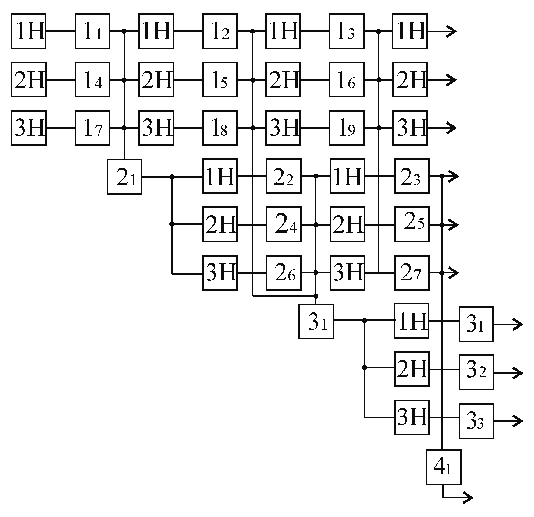
The network structure allows it to simulate the operation of a distributed computational PI network, and due to spatial separation over time, it processes information in a deterministic parallel–hierarchical network (
Figure 3). The network algorithm is universal and consists of the parallel–hierarchical formation of sets of general and various states of the spatial–temporal environment (PSE). The generalization of all types of information occurs in the final stage of the transformation.
A graphical representation is convenient for illustrating the concepts of the algorithm for operating the computational PI network, where the structure consists of sets and elements. Accordingly, the network graph contains three types of nodes. In
Figure 3, the rectangle symbol represents the initial set, the square represents the intermediate set, and the circle represents the element. Directed arcs connect sets and elements—some arcs point from sets to elements, and others point from elements to sets [
10].
The arc directed from the set to the element defines the criterion for selecting the element, while the arc from the element to the set indicates the transformation of the set. The arcs are directed, making this a directed graph, where the null set is denoted by the symbol.
This means that for each element of the graph, certain operations or transformations are defined depending on the selection of the element. This structure allows for the construction of a hierarchical model where elements have clear directions and interactions based on specified criteria, as shown in
Figure 3 [
13].
Figure 3 allows us to conclude that there are elements such as
. There are elements marked on the graph with the symbol. Each of these elements does not belong to any set, as it is uniquely selected at its level during the current cycle, does not participate in the further processing of arrays, and forms the result of the process. These elements are the terminal elements or tail elements of the computational PI network, and they generate the final output.
3. Experimental Part of G-Transformation for Computational Parallel–Hierarchical Networks
The basic concept and primary tool for constructing computational PI networks are the
G-transformations. Using the
G-transformation [
1], which occurs at each branch of the PI network, the input column matrix is transformed into a band matrix, and an array of column matrices is transformed into an array of band matrices. After several applications of the
G-transformation, the input data array is converted into an array of tail elements, which are much easier to work with.
It is necessary to address the question of information preservation during the
G-transformation: whether the information is transmitted completely without loss or the emergence of redundant information [
14].
Theorem 1. The sum of the elements of any column matrix is equal to the sum of the elements of the G-transformation of that matrix.
Case 1. The matrix consists of elements that are pairwise distinct from one another.
- 1.
Representation of a column matrix.
Let us consider a column matrix consisting of a finite number (
n) of elements:
where
are elements of the matrix.
- 2.
Renumbering of matrix µ.
Since we do not use a row order for arranging the elements of the matrix
μ, the usual notation is
—the first selected element,
—the second, and so on, with
being the last. Thus, we obtain a matrix
μ, where elements are arranged in a nondecreasing order:
where the corresponding elements
are arranged in the order of their
G-transformation [
14,
15,
16].
- 3.
Selection of elements of the matrix.
We select the first element
from matrix
, then the second element from matrix
, and so on:
From the obtained matrix, we select the second element
and write the matrix of differences between the elements of the obtained matrix with the element
[
15]. At the positions of the elements with a value of 0, we place
X:
We continue this procedure
times. In the final selection, we have the following:
It should be noted that the elements of matrix are chosen arbitrarily during the construction of the G-transformation.
- 4.
Construction of the row matrix for the G-transformation.
The first element of the
G-transformation is formed by multiplying the value of the first selected element
by the number
of nonzero elements. Similarly, the second element is the product of the value of the second selected element
and the number of nonzero elements
), excluding the element
, which is replaced with 0. The procedure continues for 0 iterations. The penultimate element of the row matrix for the
G-transformation is
, and the last one is
[
16,
17,
18,
19]. It should be noted that the number of nonzero elements is determined under the condition that matrix
consists of elements that differ pairwise in magnitude.
The case where matrix
contains elements of equal magnitude requires a separate proof. Thus, the row matrix of the
G-transformation has the following form:
Each element of the
G-transformation is formed using the recursive formula:
We show that the sum of the elements of the column matrix
is equal to the sum of the elements of the row matrix obtained from the
G-transformation [
18]. The sum of the elements of the column matrix is as follows:
The sum of the elements of the row matrix from the
G-transformation is as follows:
Expanding and grouping elements
with the same indices gives
From this, it is evident that each element
appears exactly once. Thus,
Case 2. The matrix μ contains some identical elements.
- 1.
Representation of the column matrix .
Let us consider a column matrix μ consisting of n elements and containing k identical elements, where .
- 2.
Renumbering the elements of matrix .
Since the order of elements in matrix
μ is not utilized in the construction of the
G-transformation, we renumber matrix
μ based on the order in which its elements are selected for the
G-transformation. In this case, identical elements are all selected together during the first selection of any one of them. Let the first of these identical elements be selected on the
j-th step
. Then, the
k elements
are all identical. Furthermore, the condition
is imposed to ensure valid indexing. Then, matrix
has the following look:
- 3.
Selection of elements.
We select the first element
a1 and record the matrix of differences for each element with it:
We continue this procedure for
steps. On the
j-th step, we have the following:
The next step involves selecting an element
:
The next step is to select the last element:
- 4.
Construction of G-transformation for PI networks.
The first element of the
G-transformation is formed by multiplying the first selected element
of matrix
by the number of nonzero elements. Similarly, all elements of the
G-transformation are formed up to the
j-th element, which is formed by multiplying the element
of matrix
located in the
j-th place by the number of
nonzero elements [
20]. Along with the selected element, which was in the
j-th place, all elements equal to it in magnitude are selected. Therefore, the number of remaining elements decreases not by the 1 element, but by the
k equal elements. The next element of the
G-transformation is the product of the elements of matrix
at the
place by the number
of the remaining elements [
21,
22]. The last element is the product of
and the number of
. Thus, the band matrix of the
G-transformation looks as follows:
Each element of the
G-transformation is formed according to the following recurrence formula:
which is identical to the recurrence formula for the elements of the
G-transformation of a matrix with all pairwise distinct elements [
21,
23]. The sum of the elements of the column matrix
is as follows:
The sum of the elements of the band matrix
G-transformation is as follows:
In the
G-transformation, the elements are reduced by a quantity of
. Let us consider their sum without the reduction (which equals the sum of the elements of the matrix
) and prove that it is equal to the sum of the elements of the newly formed
G-transformation [
24]. We split the sum without reduction into three sums:
Obviously,
since
. Given this, we conclude that
Conclusion. The sum of the elements of the G-transformation formed based on the matrix, which contains some number of identical elements, also equals the sum of the elements of the matrix, just as in the case with all different elements. When the G-transformation is applied to any column matrix, the sum of the elements is preserved.
4. G-Transformations Modeling
Let us consider a square matrix
A, with dimensions 4 × 4:
We split the starting matrix A into smaller ones with dimensions 2 × 2.
Let us consider, in turn, the processing of each “window” of the initial matrix A.
Input matrix:
| Iteration | G-Transformation | Shift | Tail Elements | Transposition |
| 1 | | — | — | |
| 2 | | | | |
| 3 | | | | |
| 4 | | — |
| — |
Input matrix:
| Iteration | G-Transformation | Shift | Tail Elements | Transposition |
| 1 | | — | — | |
| 2 | | | | |
| 3 | | | | |
| 4 | | — |
| — |
Input matrix:
| Iteration | G-Transformation | Shift | Tail Elements | Transposition |
| 1 | | — | — | |
| 2 | | | | |
| 3 | | | | |
| 4 | | — |
| — |
Input matrix:
| Iteration | G-Transformation | Shift | Tail Elements | Transposition |
| 1 | | — | — | |
| 2 | | | | |
| 3 | | | | |
| 4 | | — |
| — |
Let us write the obtained tail elements into a new matrix,
A*:
We divide the resulting matrix A* into “windows” according to the mathematical model above. Again, we consider the processing of each “window” of the matrix A* in turn.
Input matrix:
| Iteration | G-Transformation | Shift | Tail Elements | Transposition |
| 1 | | — | — | |
| 2 | | | | |
| 3 | | | | |
| 4 | | | | |
| 5 | | | | |
| 6 | | — |
| — |
Input matrix:
| Iteration | G-Transformation | Shift | Tail Elements | Transposition |
| 1 | | — | — | |
| 2 | | | | |
| 3 | | | | |
| 4 | | | | |
| 5 | | — |
| — |
Let us write the obtained tail elements into a new matrix
A**:
We transform the obtained matrix A** according to the mathematical model given above.
| Iteration | G-Transformation | Shift | Tail Elements | Transposition |
| 1 | | — | — | |
| 2 | | | | |
| 3 | | | | |
| 4 | | | | |
| 5 | | | | |
Tail element of PI network:
Result:


 ,
, 