Locality-Preserving Multiprojection Discriminant Analysis

Abstract

Linear discriminant analysis (LDA), as an effective feature extraction method, has been widely applied in high-dimensional data analysis. However, its discriminative performance is still severely limited by the following factors. First, the restriction on the total number of features available from LDA has seriously limited its application to problems where the feature dimension is much larger than the number of classes. Second, LDA cannot deal with data containing multiple clusters (or subclasses) within a class because it cannot correctly depict the local structure of the data. To alleviate this issue, we propose a locality-preserving multiprojection discriminant analysis (LPMDA) model to extract more discriminative features preserving local structure. Specifically, LPMDA rephrases the objective function of LDA as a convex discriminant analysis framework from the perspective of metric learning, allowing for extracting more features than the number of classes. Furthermore, an auto-optimized graph technique is also integrated into the discriminant analysis framework to explore the local structure of the data. An efficient iterative optimization algorithm is presented to solve LPMDA. Extensive experiments on several benchmark datasets confirm the effectiveness of the proposed method.

1. Introduction

Dimensionality reduction (DR) [1,2,3] is an important technique for solving the curse of the dimensionality problem by transforming the original high-dimensional features into low-dimensional features that retain the most important information, thus reducing learning complexity and memory consumption. Depending on whether label information is available, DR methods can be divided into unsupervised and supervised methods. The former learns the low-dimensional features by exploiting the topological structures of unlabeled instances. In contrast, supervised methods can fully explore potential associations between categories and features by exploiting the additional labels, resulting in more discriminative low-dimensional features [4]. Consequently, supervised DR methods are receiving increasing attention.

Linear discriminant analysis (LDA) [5], as a classical supervised DR method, has been widely applied in various fields such as face recognition [6] and seismic object detection [7,8]. LDA tries to find the optimal projection directions, which maximize the between-class variance and minimize the within-class variance in the projected space. By fine-tuning the design, some enhanced variants of LDA have been proposed. For example, Yang et al. [9] combined the adjacency graph model with LDA to improve the robustness to intraclass distributional differences and thus improve the discriminative ability for class-overlapping data. Daniela et al. [10] introduced regularization terms ($l_1$ and fused lasso penalties) into the LDA to further enhance its generalization ability to complex distributed data. Zhang et al. [11] proposed a Fisher discrimination multiple kernel dictionary learning framework to handle nonlinear features. Ju et al. [12] proposed a robust probabilistic linear discriminant analysis model by embedding a Kronecker decomposable component in the model for tensor data. Wang et al. [13] proposed a novel ratio sum formula for linear discriminant analysis, which maximizes the sum of the ratio of between-class differences to within-class differences in each dimension after projecting. Li et al. [14] presented a discriminative feature extraction model (MMC) based on the maximum margin criterion, which effectively tackles the issue of small sample size. Recently, benefiting from the powerful representation ability of deep neural networks (DNNs), deep discriminant analysis methods [15,16,17] have received increasing attention from researchers. However, they all require a large training dataset and training time, even with high-performance equipment (e.g., GPUs or TPUs). Although LDA and its variants are effective in many applications, there are two serious limitations. One is that LDA can only extract features one less than the number of classes because of the rank deficiency in the between-class scattering matrix [6,18,19,20,21]. This limitation may not be an obvious obstacle when the number of classes is large, but it becomes a fatal bottleneck when the number of classes is small, such as the odd–even recognition problem of handwritten digits in the subsequent experiments. Another limitation is that LDA can only preserve the global structure of data while ignoring the local structure of the data [22,23,24,25]. Regrettably, the distribution of real-world data is diverse, even for data in the same class. As a result, the class arithmetic mean point of each cluster might overlap, making LDA incapable of handling the multimodal data, which degrade its performance in practice.

To deal with the first problem, several recursive discriminant analysis methods and alternative metrics to LDA have been proposed. Okada et al. [26] presented a discriminant analysis with orthonormal coordinate axes (OFDAs) to extract an unlimited number of features. Xiang et al. [6] proposed a recursive Fisher linear discriminant algorithm (RFLD) to extract a greater number of features than the number of classes. Ohta et al. [27] proposed an incremental learning algorithm for RFLD, which can effectively extract the features online by recursively calculating the discriminant vectors. Li et al. [18] constructed a robust and sparse linear discriminant analysis (RSLDA) and obtained the multiple discriminant projections via a recursive procedure. In [28], the authors redefine the between-class scatter matrix using the Chernoff distance, which allows more features to be extracted. Zhu et al. [20] divided the data of each class into a set of subclasses to improve the rank deficiency problem and determined the optimal feature dimension using the leave-one-out-test criterion. However, the aforesaid recursive procedure or subclass partitioning requires additional prior knowledge and computational overhead. Zadeh et al. [29] characterized the similarity between data from the perspective of metric learning and proposed the geometric mean metric learning (GMML) model. GMML minimizes a strictly convex optimization problem that allows for efficient closed-form solutions but cannot be directly applied to feature extraction and does not consider the local structure of the data.

To solve the second problem, several methods based on preserving local manifold structures have been proposed, such as the local Fisher and the pairwise criteria [30,31]. Local Fisher discriminant analysis (LFDA) [22] uses label information to compute within- and between-class similarity and combines the ideas of FDA and LPP to learn projection matrices. Zhang et al. [32] further improved the LFDA by using the density region estimated from each class and neighborhood information. Zhu et al. [33] proposed neighborhood linear discriminant analysis (NLDA), which constructs the scatter matrices on a neighborhood of inverse nearest neighbors to represent the internal structure of instances. In [31], a pairwise formulation of LDA based on the nearest neighbor maximum projection (NMMP) is proposed. Zhou et al. [34] presented the manifold partition discriminant analysis (MPDA) model to learn a manifold subspace and generate the low-dimensional features. However, the similarity matrices used in the above method are derived from the original data and are sensitive to noise, resulting in suboptimal results.

Despite the excellent performance of the previous works in dimensionality reduction, most of them are still based on maximizing the trace ratio or difference between the between-class and within-class scatter matrices, making it difficult to effectively solve the above problems simultaneously. To this end, we propose a novel locality-preserving multiprojection discriminant analysis (LPMDA) model to extract a flexible number of discriminative features that fully explore the local structure of data. Specifically, LPMDA builds a novel convex discriminant analysis framework from a metric learning perspective that can extract the optimal number of discriminant features, breaking the limitation of the number of classes. In addition, an auto-optimized graph technique is introduced to the convex discriminant analysis framework to preserve the local structure of instances in the low-dimensional subspace. Finally, an alternating optimization strategy is used to solve the joint optimization model. The contributions of LPMDA are highlighted as follows:

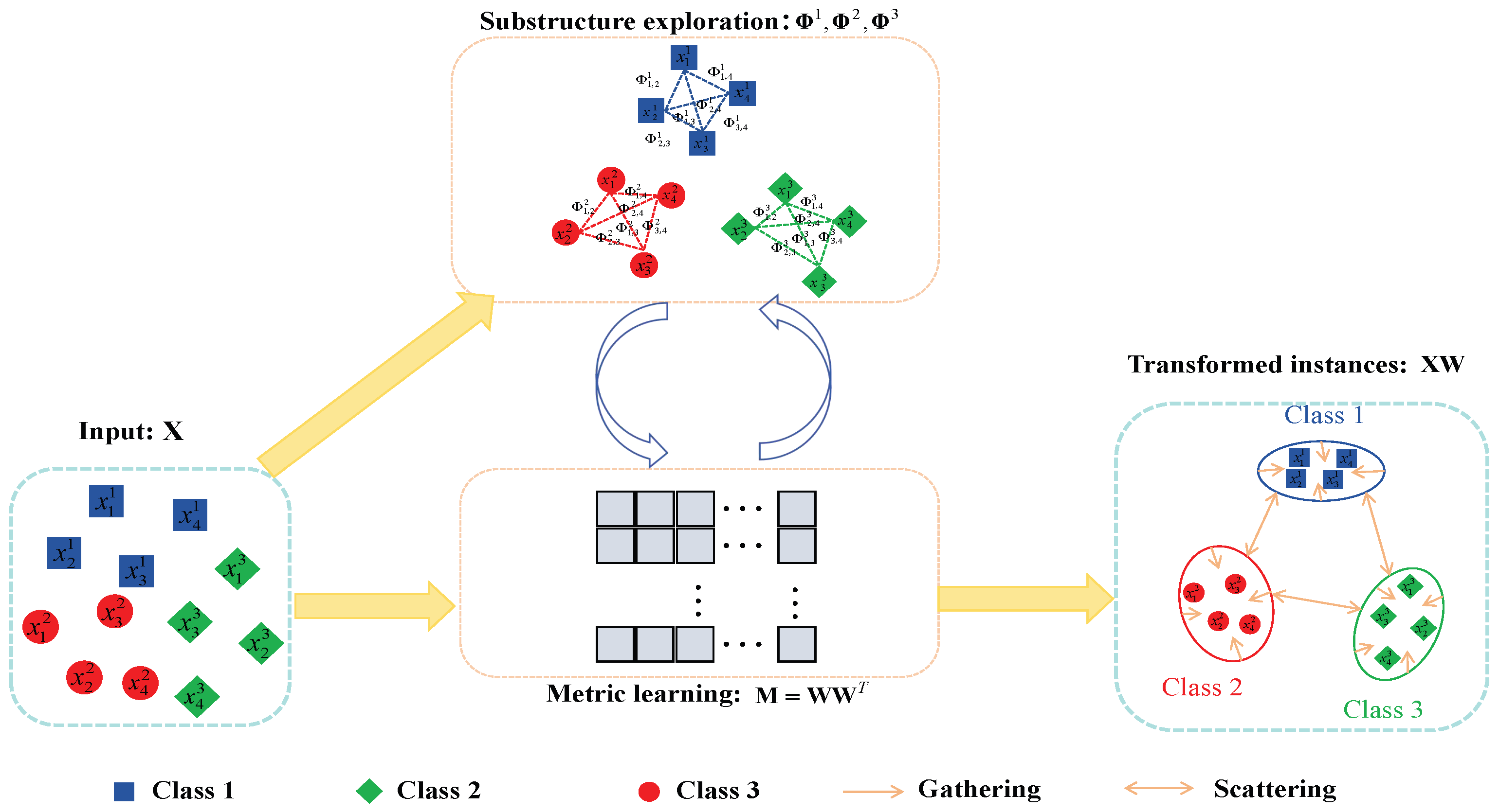
• A novel convex discriminant analysis framework is established from the perspective of metric learning, which can learn a flexible number of discriminative projections to extract more discriminative features.
• An auto-optimized graph mechanism is cleverly integrated into the discriminant analysis framework, which automatically exploits the neighborships of each instance and further enhances the discriminative ability of the extracted features.
• An efficient iterative strategy is designed to solve the resultant optimization problem. Extensive experiments were conducted on the benchmark datasets to demonstrate the superiority of the proposed method.

The rest of this article is as follows. Section 2 briefly reviews related work, including the LDA and GMML and also introduces some notations used in this article. Section 3 introduces the details of our LPMDA. Section 4 presents the experimental results and analysis. The conclusion is given in Section 5.

2. Related Works

For convenience, some notations used in this article are provided. Matrices and vectors are written in bold uppercase and bold lowercase, respectively. $\mathbf{X}={[{\mathit{x}}_1,{\mathit{x}}_2,\dots ,{\mathit{x}}_n]}^{\top }\in {\Re }^{n\times d}$ denotes a data matrix composed of n instances with d-dimensional features. Assuming that $\mathbf{X}$ can be classified into c classes, we record ${\mathbf{X}}^i={[{\mathit{x}}_1^i,{\mathit{x}}_2^i,\dots ,{\mathit{x}}_{n_i}^i]}^{\top }\in {\Re }^{n_i\times d}$ as the data submatrix with $n_i$ instances belonging to the ith class. Additionally, $\mathbf{1}$ denotes a vector with all elements that are 1. For matrix $\mathbf{M}$, $\mathrm{tr}\left(\mathbf{M}\right)$ and ${\mathbf{M}}^{-1}$ denote $\mathbf{M}$’s trace and inverse, respectively.

2.1. Linear Discriminant Analysis

LDA aims to find a low-dimensional representation of the data so that points within the same class are clustered together and points between different classes are pushed as far apart as possible. Therefore, it is easy to implement by following the trace ratio formulation:

$$\begin{array}{c}\hfill \underset{\mathbf{W}}{max}{\displaystyle \frac{Tr\left({\mathbf{W}}^{\top }{\mathbf{S}}_b\mathbf{W}\right)}{Tr\left({\mathbf{W}}^{\top }{\mathbf{S}}_w\mathbf{W}\right)}},\end{array}$$

(1)

where the optimal solution $\mathbf{W}\in {\Re }^{d\times r}$ is made of the eigenvectors corresponding to the first r largest generalized eigenvalues of ${\mathbf{S}}_w^{-1}{\mathbf{S}}_b$, if ${\mathbf{S}}_w$ is full rank. ${\mathbf{S}}_b$ and ${\mathbf{S}}_w$ denote the between-class and within-class scatter matrix, respectively, and they are defined as

$$\begin{array}{c}\hfill {\mathbf{S}}_b=\sum _{i=1}^c{n}_i({\overline{\mathit{x}}}_i-\overline{\mathit{x}}){({\overline{\mathit{x}}}_i-\overline{\mathit{x}})}^{\top },{\mathbf{S}}_w=\sum _{i=1}^c\sum _{j=1}^{n_i}({\mathit{x}}_j^i-{\overline{\mathit{x}}}_i){({\mathit{x}}_j^i-{\overline{\mathit{x}}}_i)}^{\top }\end{array}$$

(2)

Here, ${\overline{\mathit{x}}}_i$ denotes the mean instance of the ith class, and $\overline{\mathit{x}}$ is the mean instance of all data. To better figure out our method, we also reformulate the between-class and within-class scatter matrices in a pairwise manner with the following lemma.

Lemma 1. 

${\mathbf{S}}_b$ and ${\mathbf{S}}_w$ defined by (2) can be equivalently redescribed as

$$\begin{array}{c}\hfill {\mathbf{S}}_b={\displaystyle \frac{1}{2n}}\sum _{i=1}^c\sum _{k=1}^c{n}_i{n}_k({\overline{\mathit{x}}}_i-{\overline{\mathit{x}}}_k){({\overline{\mathit{x}}}_i-{\overline{\mathit{x}}}_k)}^{\top },{\mathbf{S}}_w={\displaystyle \frac{1}{2}}\sum _{i=1}^c\sum _{j=1}^{n_i}\sum _{h=1}^{n_i}{\displaystyle \frac{1}{n_i}}({\mathit{x}}_j^i-{\mathit{x}}_h^i){({\mathit{x}}_j^i-{\mathit{x}}_h^i)}^{\top }\end{array}$$

(3)

Proof. 

Please refer to Appendix A for the detailed proof of Lemma 1.    □

From (1) and (3), it can be observed that LDA faces the following two problems: (1) LDA can extract up to $c-1$ features, since the maximum rank of ${\mathbf{S}}_b$ is $c-1$; when the feature dimension is much larger than the number of classes, the discriminative performance of LDA deteriorates severely. (2) LDA only considers the global structure while overlooking the local structure of the instances; when evaluating the within-class scatter matrix (3) from a graph perspective, the graph constructed in each class is fully connected with the weights all equal to ${\displaystyle \frac{1}{n_i}}$ and thus cannot explore the local structure of the data.

2.2. Geometric Mean Metric Learning

GMML [29] seeks a metric matrix such that it yields smaller distances for similar instances and larger distances for dissimilar instances, which can be formulated as follows:

$$\begin{array}{c}\hfill \underset{\mathbf{M}\succ 0}{min}Tr\left(\mathbf{M}\mathbf{P}\right)+Tr\left({\mathbf{M}}^{-1}\mathbf{Q}\right)+\mu D_{sld}(\mathbf{M},{\mathbf{M}}_0)\end{array}$$

(4)

where $\mathbf{M}$ is a symmetric positive definite (SPD) matrix to be learned, $\mu$ is a regularization parameter, ${\mathbf{M}}_0$ is a prior SPD matrix about $\mathbf{M}$, $D_{sld}(\mathbf{M},{\mathbf{M}}_0)$ is the symmetrized LogDet divergence, and $\mathbf{P}$ and $\mathbf{Q}$ are defined as follows:

$$\begin{array}{c}\hfill \mathbf{P}={\Sigma }_{({\mathit{x}}_i,{\mathit{x}}_j)\in \mathcal{S}}({\mathit{x}}_i-{\mathit{x}}_j){({\mathit{x}}_i-{\mathit{x}}_j)}^{\top },\mathbf{Q}={\Sigma }_{({\mathit{x}}_i,{\mathit{x}}_j)\in \mathcal{D}}({\mathit{x}}_i-{\mathit{x}}_j){({\mathit{x}}_i-{\mathit{x}}_j)}^{\top }\end{array}$$

(5)

Here, $\mathcal{S}$ denotes the set of instances of the same class, and $\mathcal{D}$ denotes the set of instances from different classes. GMML tries to learn a Mahalanobis distance, i.e., find an SPD matrix $\mathbf{M}$ that yields small distances for instances in the same class. Different from most existing metric learning methods, which treat the instances of different classes asymmetrically, GMML measures the distances between the instances of different classes using ${\mathbf{M}}^{-1}$. This operation turns (4) into a strictly (geodesically) convex optimization problem and allows for a closed-form solution. For details about the strictly geodesically convex problem, this can be found in [29]. Given the excellent performance of GMML, we introduce it as a similarity measurement tool in our LPMDA.

3. Proposed Method

In this section, we propose a novel discriminant analysis framework for dimensionality reduction, which can extract more features than the number of classes, while fully preserving the local structure between instances. The proposed LPMDA mainly consists of two basic modules, i.e., multiprojection learning with adaptive metric learning and local structure exploration with auto-optimized graphs. Figure 1 illustrates the overall framework of our proposed method. The technical details of each component are detailed as follows.

3.1. Multiprojection Discriminant Analysis

As mentioned above, it is difficult to extract enough discriminative features by extension directly from LDA. To address this problem, we make a simple but crucial transformation to the optimization problem of LDA. According to the properties of the trace operation, the optimization objective (1) can be reformulated as

$$\begin{array}{c}\hfill \underset{\mathbf{W}}{max}{\displaystyle \frac{Tr\left(\mathbf{W}{\mathbf{W}}^{\top }{\mathbf{S}}_b\right)}{Tr\left(\mathbf{W}{\mathbf{W}}^{\top }{\mathbf{S}}_w\right)}},\end{array}$$

(6)

To generate multiple discriminant projections for each instance, we first introduce an SPD matrix $\mathbf{M}\in {\Re }^{d\times d}$ to replace $\mathbf{W}{\mathbf{W}}^{\top }$ in (6) and obtain

$$\begin{array}{c}\hfill \underset{\mathbf{M}\succ 0}{max}{\displaystyle \frac{Tr\left(\mathbf{M}{\mathbf{S}}_b\right)}{Tr\left(\mathbf{M}{\mathbf{S}}_w\right)}}.\end{array}$$

(7)

It should be noted that optimization problem (7) is not convex with respect to $\mathbf{M}$, and solving it usually involves iterative techniques, leading to considerable computational complexity. To maximize the variance of the intraclass class while maximizing those of the interclass, we embed a metric matrix $\mathbf{M}$ in the numerator term and its inverse matrix ${\mathbf{M}}^{-1}$ in the denominator term of (7), respectively, and sum them. Therefore, it becomes

$$\begin{array}{c}\hfill \underset{\mathbf{M}\succ 0}{min}Tr\left(\mathbf{M}{\mathbf{S}}_w\right)+Tr\left({\mathbf{M}}^{-1}{\mathbf{S}}_b\right)+\mu D_{sld}(\mathbf{M},{\mathbf{M}}_0).\end{array}$$

(8)

where $\mu$ is a regularization parameter, ${\mathbf{M}}_0$ is the prior knowledge of the SPD matrix, and $D_{sld}(\mathbf{M},{\mathbf{M}}_0)$ is the symmetrized LogDet divergence [29], i.e.,

$$\begin{array}{c}\hfill D_{sld}(\mathbf{M},{\mathbf{M}}_0)=tr\left(\mathbf{M}{\mathbf{M}}_0^{-1}\right)+tr\left({\mathbf{M}}^{-1}{\mathbf{M}}_0\right)-2d\end{array}$$

(9)

Replacing the tracking ratio operation in (7) with the asymmetric operation in GMML [29] effectively avoids the rank deficiency in between-class scattering and thus yields more discriminative projections. Model (8) aims to find a metric space measured by $\mathbf{M}$ such that instances of each class are close to the class centroid while the centroids of different classes are far apart in this metric space. Our goal is to obtain the multiple discriminant projections for each instance, which is nothing but the Cholesky decomposition of $\mathbf{M}$. Therefore, the goal of model (8) fully aligns with the core motivation of LDA but can extract any number of discriminative features. This is a breakthrough improvement over the original LDA. It is worth noting that the metric matrix $\mathbf{M}$ in our model is essentially different from that in GMML. This is because ${\mathbf{S}}_w$ and ${\mathbf{S}}_b$ in (8) are only the within-class scatter matrix and the between-class scatter matrix, whereas $\mathbf{P}$ and $\mathbf{Q}$ in (4) are scaled second sample moments of the differences between similar instances and the differences between dissimilar instances. Therefore, model (8) provides a more refined description of data distribution and class information.

3.2. Local Structure Exploitation

Referring to Equation (3), classical LDA methods calculate the within-class scatter matrix ${\mathbf{S}}_w$ using a fully connected equal-weight graph, which cannot explore the local geometric structure of the instances. To this end, we embed an auto-optimized graph into the within-class scatter to adaptively exploit the local geometric structure of the instances as follows:

$$\begin{array}{c}\hfill {\tilde{\mathbf{S}}}_w=\sum _{i=1}^c\sum _{j=1}^{n_i}\sum _{h=1}^{n_i}{\displaystyle \frac{{\mathbf{\Phi }}_{j,h}^i}{n_i}}({\mathit{x}}_j^i-{\mathit{x}}_h^i){({\mathit{x}}_j^i-{\mathit{x}}_h^i)}^{\top },s.t.{\mathbf{\Phi }}_{j,:}^i\mathbf{1}=k,{\mathbf{\Phi }}_{j,h}^i\in \{0,1\},\end{array}$$

(10)

where ${\mathbf{\Phi }}_{j,h}^i$ is a kNN graph to be learned, which can be viewed as the weight between ${\mathit{x}}_j^i$ and ${\mathit{x}}_h^i$, and ${\mathbf{\Phi }}_{j,:}^i$ denotes the weights of ${\mathit{x}}_j^i$. In short, the kNN graph $\mathbf{\Phi }$ can be automatically optimized, and the optimal neighborships between instances can be found as the algorithm converges, thus exploring the submanifold structure of the instances.

3.3. Objective Function

By incorporating both the multiprojection discriminant analysis and local structure exploitation, we remodel LDA and achieve the objective of the proposed LPMDA as

$$\begin{array}{c}\hfill \underset{\mathbf{M}\succ 0}{min}Tr\left(\mathbf{M}{\tilde{\mathbf{S}}}_w\right)+Tr\left({\mathbf{M}}^{-1}{\tilde{\mathbf{S}}}_b\right)+\mu D_{sld}(\mathbf{M},{\mathbf{M}}_0),s.t.{\mathbf{\Phi }}_{j,:}^i\mathbf{1}=k,{\mathbf{\Phi }}_{j,h}^i\in \{0,1\}\end{array}$$

(11)

The proposed model (11) is more appealing than the LDA on the basis of the following two considerations. First, the total number of features available in LPMDA is independent of the number of classes, thus overcoming the major drawback that the total number of features available from LDA is limited to the number of classes minus one. Second, LPMDA embeds an auto-optimized k-nearest neighbor graph in the framework, which allows the model to fully exploit not only the differences between instances from different classes but also the local structural information between instances from the same class, further enhancing the discriminativeness of the extracted features. Model (11) combines metric learning and adaptive graph learning to construct a unified discriminant analysis framework, which can also be refined by introducing more sophisticated tricks such as nonlinear metric learning and hypergraph learning.

3.4. Optimization for LPMDA

In this section, we present an iterative optimization algorithm to solve problem (11). First, the distance matrix in the original space is calculated by Euclidean distance, and the similarity matrix $\mathbf{\Phi }$ is initialized by the rule that if instance ${\mathit{x}}_h^i$ is the kNN point of ${\mathit{x}}_j^i$, then the element ${\mathbf{\Phi }}_{j,h}^i$ is equal to 1; otherwise, it is 0. We will then iteratively optimize $\mathbf{M}$ and $\mathbf{\Phi }$ as follows.

When fixing $\mathbf{\Phi }$, $\mathbf{M}$ is updated by solving the following problem:

$$\underset{\mathbf{M}\succ 0}{min}Tr\left(\mathbf{M}{\tilde{\mathbf{S}}}_w\right)+Tr\left({\mathbf{M}}^{-1}{\tilde{\mathbf{S}}}_b\right)+\mu D_{sld}(\mathbf{M},{\mathbf{M}}_0).$$

(12)

The optimal solution of (12) is the midpoint of the geodesic joining ${\tilde{\mathbf{S}}}_w^{-1}$ to ${\tilde{\mathbf{S}}}_b$ [35]; that is,

$$\mathbf{M}={({\tilde{\mathbf{S}}}_w+\mu {\mathbf{M}}_0^{-1})}^{-1}{♯}_{\alpha }({\tilde{\mathbf{S}}}_b+\mu {\mathbf{M}}_0),$$

(13)

where ${♯}_{\alpha }(·)$ is defined as $\mathbf{A}{♯}_{\alpha }\mathbf{B}={\mathbf{A}}^{1/2}{\left({\mathbf{A}}^{-1/2}\mathbf{B}{\mathbf{A}}^{-1/2}\right)}^{\alpha }{\mathbf{A}}^{1/2}$, and $\alpha \in (0,1)$ is a weighting parameter.

When fixing $\mathbf{M}$, $\mathbf{\Phi }$ is updated by solving the following problem:

$$\begin{array}{c}\hfill \underset{\mathbf{\Phi }}{min}\sum _{i=1}^c{\displaystyle \frac{1}{n_i}}\sum _{j=1}^{n_i}\sum _{h=1}^{n_i}{\mathbf{\Phi }}_{j,h}^{i}Tr\left(\mathbf{M}({\mathit{x}}_j^i-{\mathit{x}}_h^i){({\mathit{x}}_j^i-{\mathit{x}}_h^i)}^{\top }\right),s.t.{\mathbf{\Phi }}_{j,:}^i\mathbf{1}=k,{\mathbf{\Phi }}_{j,h}^i\in \{0,1\}\end{array}$$

(14)

which is equivalent to solving the following subproblem:

$$\begin{array}{c}\hfill \underset{{\mathbf{\Phi }}_{j,:}^i}{min}\sum _{h=1}^{n_i}{\mathbf{\Phi }}_{j,h}^i{\parallel {\mathit{x}}_j^i-{\mathit{x}}_h^i\parallel }_{\mathbf{M}}^2,s.t.{\mathbf{\Phi }}_{j,:}^i\mathbf{1}=k,{\mathbf{\Phi }}_{j,h}^i\in \{0,1\},\end{array}$$

(15)

where ${\parallel {\mathit{x}}_j^i-{\mathit{x}}_h^i\parallel }_{\mathbf{M}}^2={({\mathit{x}}_j^i-{\mathit{x}}_h^i)}^{\top }\mathbf{M}({\mathit{x}}_j^i-{\mathit{x}}_h^i)$ denotes the square Mahalanobis distance between ${\mathit{x}}_j^i$ and ${\mathit{x}}_h^i$. It is obvious that there are only k elements equal to 1 in the vector ${\mathbf{\Phi }}_{j,:}^i$, and the others are all 0, because of the constraints on ${\mathbf{\Phi }}_{j,:}^i$. Assuming that the indices of the non-zero elements in the vector ${\mathbf{\Phi }}_{j,:}^i$ are $\{{\tau }_1,{\tau }_2,\dots ,{\tau }_m,\dots ,{\tau }_k\}(1\le {\tau }_m\le n_i,{\tau }_m\ne j)$, then problem (15) can be reduced as

$$\begin{array}{c}\hfill \underset{{\tau }_m}{min}\sum _{m=1}^k{\parallel {\mathit{x}}_j^i-{\mathit{x}}_{{\tau }_m}^i\parallel }_{\mathbf{M}}^2.\end{array}$$

(16)

Obviously, the optimal solution ${\tau }_m^{*}$ of problem (16) is the indices of the instances of the kNNs of ${\mathit{x}}_j^i$ under the Mahalanobis distance based on $\mathbf{M}$. Then, the optimal solution to (15) is

$${\mathbf{\Phi }}_{j,h}^i=\left\{\begin{array}{cc}1\hfill & \mathrm{if}h={\tau }_m^{*}\hfill \\ 0\hfill & \mathrm{otherwise}\hfill \end{array}\right.,$$

(17)

which is consistent with the motivation to find neighbors in the optimal subspace to eliminate the effects of noise.

Following the iterative optimization of $\mathbf{M}$ and $\mathbf{\Phi }$, our method is able to automatically assign k optimal neighbors to each instance. Based on the optimal $\mathbf{M}$, we can obtain the projection matrix $\mathbf{W}$ with flexible dimensionality and the capability to preserve the local structure of the instances, which is exactly the Cholesky decomposition of $\mathbf{M}$, i.e., satisfying $\mathbf{M}=\mathbf{W}{\mathbf{W}}^{\top }$. Algorithm 1 summarizes the procedure of LPMDA in which the convergence condition used in our experiments is ${\displaystyle \frac{\parallel {\mathbf{W}}^{k+1}-{\mathbf{W}}^k{\parallel }_F}{\parallel {\mathbf{W}}^k{\parallel }_F}}\le {10}^{-4}$.

Algorithm 1 Algorithm for solving LPMDA

Input: Training instance matrix $\mathbf{X}$, label matrix $\mathbf{Y}$, regularization parameter $\mu$, weighting parameter $\alpha \in (0,1)$, neighbors number k, reduced dimension r. Initialization:  $\mathbf{\Phi }\in {\Re }^{n\times n}$ While not converged do 1. Update $\mathbf{M}$ by solving problem (12) 2. Calculate $\mathbf{\Phi }$ according to Equation (15). end while $\mathbf{W}:=Chol\left(\mathbf{M}\right)$, where $Chol(·)$ denotes the Cholesky decomposition operation. Output: $\mathbf{W}\in {\Re }^{d\times r}$.

3.5. Complexity and Convergence Analysis

Obviously, the cost of LPMDA consists of two parts. The first part is to find the SPD matrix $\mathbf{M}$, which requires the Cholesky decomposition of ${\tilde{\mathbf{S}}}_b$ and ${\tilde{\mathbf{S}}}_w$, with a complexity of approximately $O\left(d^3\right)$. The second part is to solve $\mathbf{\Phi }$, which only involves some basic operations such as vector subtraction and multiplication, which can be ignored compared to the first part. Thus, the total computational complexity of LPMDA is $O\left(t{d}^3\right)$, where t is the number of iterations. For a more detailed comparison,

Table 1. Time complexity of the comparison methods, where t denotes the number of iterations, and $N_p$ is the number of submanifold partitions in MPDA.

Method	Computational Complexity
LDA [21]	$O(n{d}^2+d^3)$
MMC [14]	$O(n{d}^2+t{d}^3)$
NMMP [31]	$O(n^{2}d+tnrd)$
RFLD [6]	$O\left(t(n{d}^2+d^3)\right)$
RSLDA [18]	$O(n^3+tn{c}^2)$
MPDA [34]	$O({(n+d)}^3+{\sum }_{p=1}^P(d^2{N}_p+N_p^{2}d))$
NLDA [33]	$O(n^2+d^3)$
LPMDA	$O\left(t{d}^3\right)$

reports the time complexity of the comparison methods in this paper. It is obvious that our model will eventually converge to a local optimum, since the optimal solution can be obtained at each optimization step.

3.6. Connections to Previous Discriminators

To provide a deeper insight into our approach, this section details the differences between our LPMDA and several closely related discriminators. Indeed, most existing discriminators can be unified into the following framework:

$$\begin{array}{c}\hfill \underset{\mathbf{W}}{min}\mathcal{L}({\mathbf{S}}_b,{\mathbf{S}}_w,\mathbf{W})s.t.\mathbf{W}\in \mathsf{\Omega }\end{array}$$

(18)

where $\mathcal{L}(·)$ denotes the optimization criterion; ${\mathbf{S}}_b$ and ${\mathbf{S}}_w$ are the generalized between- and within-class scatter matrices of instances, respectively, which may be defined differently in different methods; $\mathbf{W}$ is the projection matrix; and $\mathsf{\Omega }$ denotes the constraint for $\mathbf{W}$.

Table 2. Descriptions of representative advanced discriminators and our LPMDA based on framework (18). ‘♯ Features’ denotes the maximum number of available features, ${\overline{\mathit{x}}}_i$ and $\overline{\mathit{x}}$ are the mean vectors of ${\mathbf{X}}^i$ and $\mathbf{X}$, and $N{N}_k\left(\mathit{x}\right)$ denotes the k-nearest neighbors of $\mathit{x}$.

Methods	$\mathcal{L}(\mathbf{X},\mathbf{Y},\mathbf{W},\mathbf{V})$	Definition of ${\mathit{S}}_{\mathit{b}}$ and ${\mathit{S}}_{\mathit{w}}$	♯ Features	Structure Preservation
LDA [21]	$\mathbf{W}=arg\underset{\mathbf{W}}{max}{\displaystyle \frac{Tr\left({\mathbf{W}}^{\top }{\mathbf{S}}_b\mathbf{W}\right)}{Tr\left({\mathbf{W}}^{\top }{\mathbf{S}}_w\mathbf{W}\right)}}$	${\mathbf{S}}_b={\displaystyle \sum _{i=1}^c}{n}_i({\overline{\mathit{x}}}_i-\overline{\mathit{x}}){({\overline{\mathit{x}}}_i-\overline{\mathit{x}})}^{\top }$ ${\mathbf{S}}_w={\displaystyle \sum _{i=1}^c\sum _{j=1}^{n_i}}({\mathit{x}}_j^i-{\overline{\mathit{x}}}_i){({\mathit{x}}_j^i-{\overline{\mathit{x}}}_i)}^{\top }$	$\le c-1$	global
MMC [14]	$\mathbf{W}=arg\underset{{\mathbf{W}}^{\top }\mathbf{W}=\mathbf{I}}{max}Tr\left({\mathbf{W}}^{\top }({\mathbf{S}}_b-{\mathbf{S}}_w)\mathbf{W}\right)$	${\mathbf{S}}_b={\displaystyle \sum _{i=1}^c}{n}_i({\overline{\mathit{x}}}_i-\overline{\mathit{x}}){({\overline{\mathit{x}}}_i-\overline{\mathit{x}})}^{\top }$ ${\mathbf{S}}_w={\displaystyle \sum _{i=1}^c\sum _{j=1}^{n_i}}({\mathit{x}}_j^i-{\overline{\mathit{x}}}_i){({\mathit{x}}_j^i-{\overline{\mathit{x}}}_i)}^{\top }$	$\ge c$	global
RFLD [6]	${\mathit{w}}^{(k+1)}=arg\underset{{\mathit{w}}^{\top }{\mathit{w}}^{\left(k\right)}=1}{max}{\displaystyle \frac{{\mathit{w}}^{\top }{\mathbf{S}}_b^{\left(k\right)}\mathit{w}}{{\mathit{w}}^{\top }{\mathbf{S}}_w^{\left(k\right)}\mathit{w}}}$	${\mathit{x}}_i^{(k+1)}={\mathit{x}}_i^{\left(k\right)}-{{\mathit{w}}^{\left(k\right)}}^{\top }{\mathit{x}}_i^{\left(k\right)}{\mathit{w}}^{\left(k\right)}$ ${\mathbf{S}}_b^{(k+1)}={\displaystyle \sum _{i=1}^c}{n}_i({\overline{\mathit{x}}}_i^{(k+1)}-{\overline{\mathit{x}}}^{(k+1)}){({\overline{\mathit{x}}}_i^{(k+1)}-{\overline{\mathit{x}}}^{(k+1)})}^{\top }$ ${\mathbf{S}}_w^{(k+1)}={\displaystyle \sum _{i=1}^c\sum _{j=1}^{n_i}}({{\mathit{x}}_j^i}^{(k+1)}-{\overline{\mathit{x}}}_i^{(k+1)}){({{\mathit{x}}_j^i}^{(k+1)}-{\overline{\mathit{x}}}_i^{(k+1)})}^{\top }$	$\ge c$	global
RSLDA [18]	${\mathit{w}}^{(k+1)}=arg\underset{\mathit{w}}{min}-{\displaystyle \sum _{i=1}^c}{n}_i|{\mathit{w}}^{\top }{\mathit{x}}_i^{(k+1)}-{\overline{\mathit{x}}}^{(k+1)}|$ $+\lambda {\mathit{w}}^{\top }{\mathbf{S}}_w^{(k+1)}\mathit{w}+\delta {\parallel \mathit{w}\parallel }_1$	${\mathit{x}}_i^{(k+1)}={\mathit{x}}_i^{\left(k\right)}-\sum _{j=1}^k{{\mathit{w}}^{\left(j\right)}}^{\top }{\mathit{x}}_i^{\left(k\right)}{\mathit{w}}^{\left(j\right)}$ ${\mathbf{S}}_w^{(k+1)}=\sum _{i=1}^c\sum _{j=1}^{n_i}({{\mathit{x}}_j^i}^{(k+1)}-{\overline{\mathit{x}}}_i^{(k+1)}){({{\mathit{x}}_j^i}^{(k+1)}-{\overline{\mathit{x}}}_i^{(k+1)})}^{\top }$	$\ge c$	global
NMMP [31]	$\mathbf{W}=arg\underset{{\mathbf{W}}^{\top }\mathbf{W}=\mathbf{I}}{max}{\displaystyle \frac{Tr\left({\mathbf{W}}^{\top }{\mathbf{S}}_b\mathbf{W}\right)}{Tr\left({\mathbf{W}}^{\top }{\mathbf{S}}_w\mathbf{W}\right)}}$	${\mathcal{N}}_b\left(C_j\right)=\left\{{\mathit{x}}_q\right|{\mathit{x}}_q\in N{N}_k\left({\mathit{x}}_j\right),C_q\ne C_j\}$ ${\mathcal{N}}_w\left(C_j\right)=\left\{{\mathit{x}}_q\right|{\mathit{x}}_q\in N{N}_k\left({\mathit{x}}_j\right),C_q=C_j\}$ ${\mathbf{S}}_b={\displaystyle \sum _{i,j:{\mathit{x}}_i\in {\mathcal{N}}_b\left(C_j\right)\&{\mathit{x}}_j\in {\mathcal{N}}_b\left(C_i\right)}}({\mathit{x}}_i-{\mathit{x}}_j){({\mathit{x}}_i-{\mathit{x}}_j)}^{\top }$ ${\mathbf{S}}_w={\displaystyle \sum _{i,j:{\mathit{x}}_i\in {\mathcal{N}}_w\left(C_j\right)\&{\mathit{x}}_j\in {\mathcal{N}}_w\left(C_i\right)}}({\mathit{x}}_i-{\mathit{x}}_j){({\mathit{x}}_i-{\mathit{x}}_j)}^{\top }$	$\ge c$	local
NLDA [33]	$\mathbf{W}=arg\underset{\mathbf{W}}{max}Tr\left({\left({\mathbf{W}}^{\top }{\mathbf{S}}_w\mathbf{W}\right)}^{-1}\left({\mathbf{W}}^{\top }{\mathbf{S}}_b\mathbf{W}\right)\right)$	$RN{N}_k({\mathit{x}}_i,\mathbf{X})=\left\{{\mathit{x}}_q\right|{\mathit{x}}_q\in \mathbf{X}{\mathit{x}}_i,{\mathit{x}}_i\in N{N}_k\left({\mathit{x}}_q\right)\}$ ${\mathit{m}}_i={\displaystyle \frac{1}{|RN{N}_k({\mathit{x}}_i,{\mathbf{X}}_{y_i})|}}{\displaystyle \sum _{{\mathit{x}}_j\in RN{N}_k({\mathit{x}}_i,{\mathbf{X}}_{y_i})}}{\mathit{x}}_j$ ${\mathbf{S}}_b={\displaystyle \sum _{i=1,|RN{N}_k({\mathit{x}}_i,{\mathbf{X}}_{y_i})|\ge t}^n\sum _{j=1,|RN{N}_k({\mathit{x}}_j,{\mathbf{X}}_{y_j})|\ge t,y_i\ne y_j}^n}({\mathit{m}}_i-{\mathit{m}}_j){({\mathit{m}}_i-{\mathit{m}}_j)}^{\top }$ ${\mathbf{S}}_w={\displaystyle \sum _{i=1,|RN{N}_k({\mathit{x}}_i,{\mathbf{X}}_{y_i})|\ge t}^n\sum _{{\mathit{x}}_j\in RN{N}_k({\mathit{x}}_i,{\mathbf{X}}_{y_i})}}({\mathit{x}}_j-{\mathit{m}}_i){({\mathit{x}}_j-{\mathit{m}}_i)}^{\top }$	$\ge c$	local
LPMDA	$\mathbf{M}=arg\underset{\mathbf{M}\succ 0,\mathbf{\Phi }}{min}Tr\left(\mathbf{M}{\tilde{\mathbf{S}}}_w\right)+Tr\left({\mathbf{M}}^{-1}{\tilde{\mathbf{S}}}_b\right)$ $+\mu D_{sld}(\mathbf{M},{\mathbf{M}}_0)$	${\tilde{\mathbf{S}}}_b={\displaystyle \frac{1}{2n}}{\sum }_{i=1}^c{\sum }_{k=1}^c{n}_i{n}_k({\overline{\mathit{x}}}_i-{\overline{\mathit{x}}}_k){({\overline{\mathit{x}}}_i-{\overline{\mathit{x}}}_k)}^{\top }$ ${\tilde{\mathbf{S}}}_w={\sum }_{i=1}^c{\sum }_{j=1}^{n_i}{\sum }_{h=1}^{n_i}{\displaystyle \frac{{\mathbf{\Phi }}_{j,h}^i}{n_i}}({\mathit{x}}_j^i-{\mathit{x}}_h^i){({\mathit{x}}_j^i-{\mathit{x}}_h^i)}^{\top }$ ${\mathbf{\Phi }}_{j,:}^i\mathbf{1}=k,{\mathbf{\Phi }}_{j,h}^i\in \{0,1\}$	$\ge c$	local

summarizes some representative methods and our LPMDA in the form of framework (18). These methods typically improve feature extraction from the following two core points: (1) Designing different optimization criteria or iterative strategies to extract more features. For example, MMC [14] avoids the small sample size problem by employing the maximum margin criterion; RFLD [6] and RSLDA [18] extract more discriminative features using an iterative strategy. (2) Embedding graph similarity or neighborhood information in the scatter matrix to fully exploit the local structure of instances. For example, NMMP [31], NLDA [33], and MPDA [34] introduce graph similarity into the scatter matrix to fully exploit the local structure of instances. Our LPMDA starts from a new perspective of metric learning, incorporating adaptive graph learning to extract more discriminative features, taking into account local information, without requiring iterative learning.

4. Experiments

In this section, LPMDA is compared with several representative related methods, including classical LDA [21], MMC [14], RFLD [6], and RSLDA [18], which can extract more features than the number of classes, and NMMP [31], NLDA [33], and MPDA [34], which take into account the local structure of the sample. All parameters of the comparative methods were set according to the suggestions of the relevant literature. In our LPMDA, the regularization parameter $\mu$ is set to $\mu ={10}^{-4}$ to avoid matrix singularity, $\alpha \in (0,1)$ is the weighting parameter and is selected from the set $\{{10}^{-6},{10}^{-5},\dots ,{10}^{-2}\}$, and the number of neighbors per class k is set to 5. The prior matrix ${\mathbf{M}}_0$ was set to the identity matrix throughout the experiment. All the parameters in these models are selected from their own candidate set by the five-fold cross-validation technique on the corresponding training datasets. First, we evaluate the ability of LPMDA to explore the local structural information of instances in multimodal classes. Specifically, two handwritten digit recognition datasets are used to identify whether a digit is odd or even. Then, we further evaluate LPMDA on six public benchmark datasets, for which we do not know whether they contain a multimodal class or not.

All experiments are run 10 times with random data splits of training and test samples, and then the mean classification results with standard deviation are reported on different datasets. All experiments are implemented on MATLAB R2017a with Win7 system, Inter Core i7-8550 CPU, and 8 GB RAM.

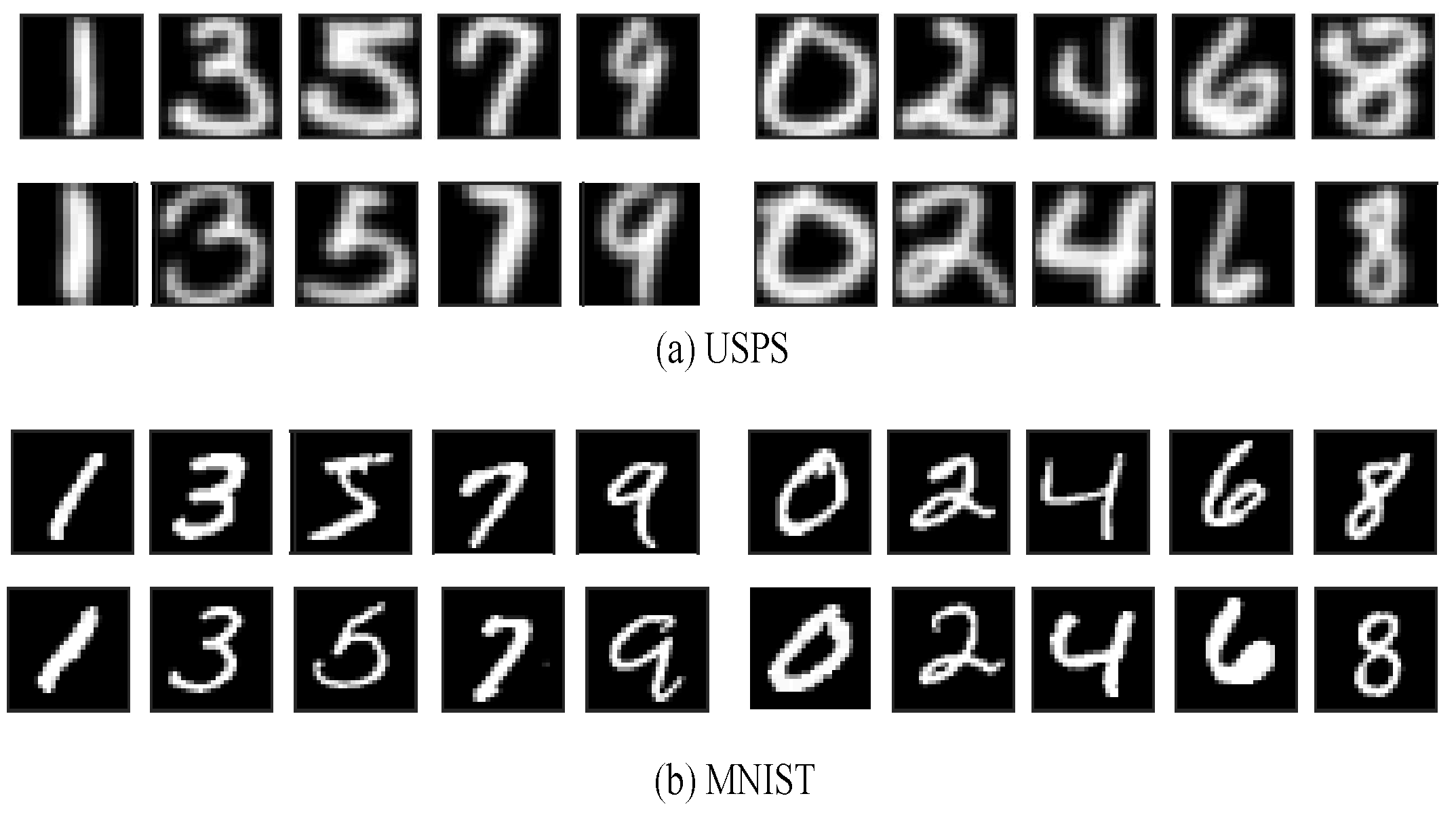
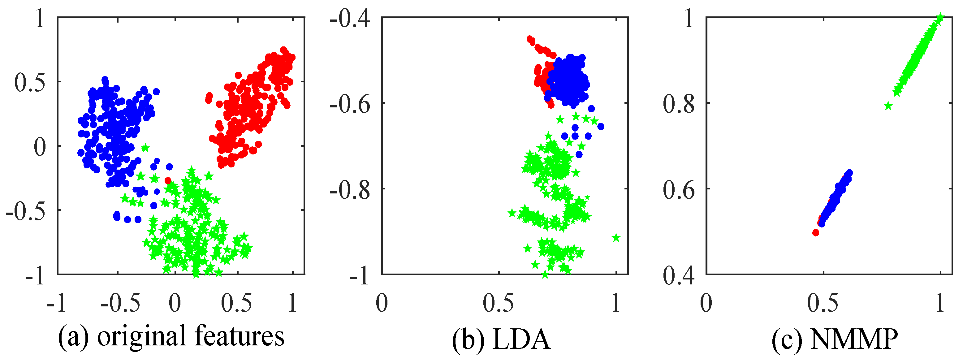
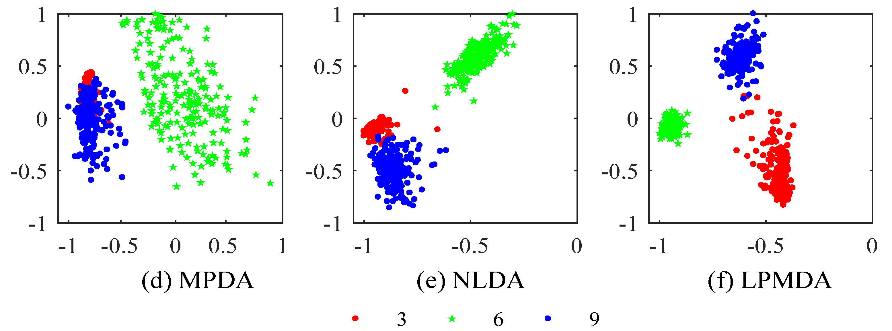
4.1. Experiments on Handwritten Digit Recognition

In this subsection, we will use two handwritten digit datasets, including USPS and MNIST, to evaluate the proposed method. The details of these datasets are given in

Table 3. Brief description of the handwritten digit datasets.

Class	USPS		MNIST
	♯Training	♯Test	♯Training	♯Test
0	644	177	5923	980
1	1194	359	6742	1135
2	1005	264	5958	1032
3	731	198	6131	1010
4	658	166	5842	982
5	652	200	5421	892
6	556	160	5918	958
7	664	170	6265	1028
8	645	147	5851	974
9	542	166	5949	1009

, where ♯ indicates the corresponding number of instances. For each dataset, we aim to identify whether the digit is odd or even. Therefore, handwritten digit recognition is transformed into a binary classification problem, where each class consists of five subclasses, and some digital images are shown in Figure 2.

In these experiments, each gray image is resized to $16\times 16$ with 256-D features. For fair comparison, the reduced dimensions of LDA are set to $c-1$ ($c=2$), and the optimal dimensions of other methods are searched from [10:10:200]. All the experiments are repeated 20 times. Finally, the average classification accuracies with standard deviations are reported in

Table 4. Experimental results (%) (best average accuracy ± standard deviations (%); optimal reduced dimensions) on handwritten digit datasets; the best results are highlighted in bold.

Data	LDA	MMC	NMMP	RFLD	RSLDA	MPDA	NLDA	LPMDA
USPS	94.02 ± 1.21	95.33 ± 1.33	96.73 ± 1.51	96.55 ± 1.31	97.21 ± 1.51	98.01 ± 1.62	97.21 ± 1.55	98.89 ± 0.81
	(1)	(140)	(160)	(160)	(130)	(110)	(160)	(150)
MNIST	83.18 ± 1.66	84.52 ± 1.73	85.67 ± 1.55	85.72 ± 1.45	87.32 ± 1.62	88.53 ± 1.71	87.51 ± 1.60	89.75 ± 0.85
	(1)	(120)	(130)	(140)	(110)	(100)	(130)	(140)

. From Table 4, we can see that LDA performs poorly on these two datasets, mainly because each class is multimodal and contains five subclasses, while LDA does not consider the local structure between instances. In addition, the number of features generated by LDA is much smaller than the feature dimension, which is another major reason for its performance degradation. Two locality-preserved methods including NMMP and NLDA outperform LDA and MMC, confirming the need to explore the local structure to discriminate the multimodal data. LPMDA achieves the best performance among all the comparison methods. Specifically, for the USPS data, the accuracy of LPMDA improves by 4.87% over DLSR; about 3.56% over MMC; about more 2% over NMMP, RFLD and RSLDA; about more 1% over NLDA; and about 0.88% over the best competitor, MPDA. For MNIST data, LPMDA increased by 6.57% compared to LDA, 5.23% compared to MMC, and even more compared to NMMP; RFLD increased by more than 4%, which is more than 2% higher than RSLDA and NLDA, and about 1.22% higher than the best competitor, MPDA. This is because LPMDA can extract enough discriminative features that preserve the local structure of the instances.

To further validate the ability of our model LPMDA to capture local structures between instances, we conducted a 2-D visualization experiment on a subset of the USPS, which merges the ‘3’ and ‘9’ into an odd class (‘•’ and ‘•’) and denotes the ‘6’ as the even class (‘★’). We compare the embedding results of LPMDA with those of LDA, NMMP, MPDA, NLDA, and evaluate the between-class separability (i.e., ‘•’ and ‘•’ are well separated from ‘★’) and the within-class multimodality preservation ability (i.e., ‘•’ and ‘•’ are well grouped). Figure 3 shows the instances embedded in the two-dimensional space found by each method. The horizontal axis is the first feature found by each method, while the vertical axis is the second feature. LDA allows us to extract only one meaningful feature in binary class classification problems (see Section 2.1), so here, we choose the second feature at random. We also visualize the t-SNE of the original features [36] as a reference. From Figure 3, we can see that LDA tends to mix instances from different classes, which would be caused by the within-class multimodality. NMMP and MPDA separate ‘•’ and ‘•’ from ‘★’ well, but the within-class multimodality is lost, i.e., ‘•’ and ‘•’ are mixed. NLDA separates odd classes from even classes well and preserves the within-class multimodality to some extent. LPMDA nicely separates instances in different classes from each other, while clearly preserving the within-class multimodality.

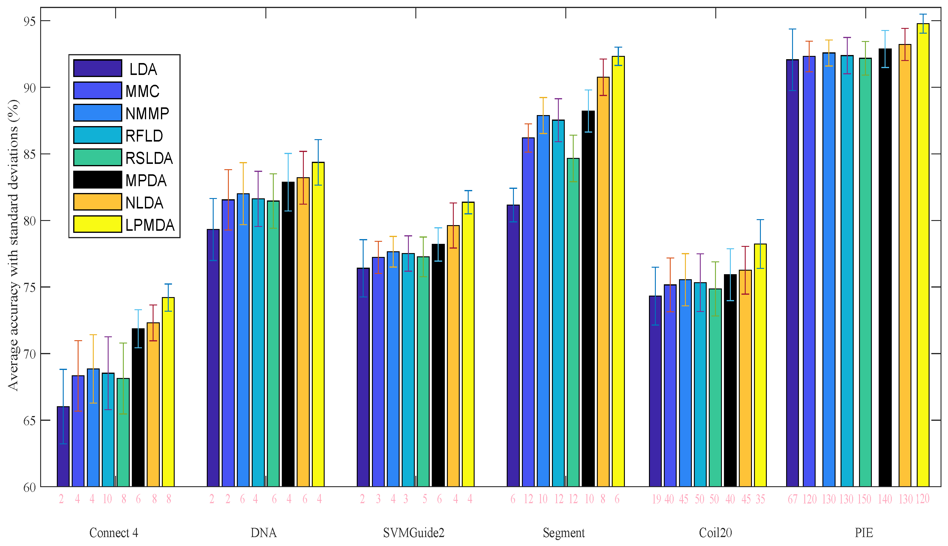
4.2. Experiments on Benchmark Datasets

In this subsection, we use four datasets, i.e., Connect 4, DNA, SVMGuide2, and Segment, which are available from the UCI database website, as well as one object data Coil20 and one face image dataset PIE [37], to evaluate the proposed discriminator. The PIE face dataset contains 68 people with 41368 face images in total. We select a subset of this dataset, where each person has 170 images that are collected under five different poses (C05, C07, C09, C27, and C29). The details of these datasets are listed in

Table 5. Brief description of the benchmark datasets used in experiments.

Dataset	# Classes	# Instances	# Features
Connect 4	3	44,473	126
DNA	3	3186	180
SVMGuide2	3	391	20
Segment	7	2310	19
Coil20	20	1440	256
PIE	68	11,554	1024

. The number of classes ranges from 3 to 68. The number of features ranges from 19 to 1024. The reduced dimensions of LDA are set to $c-1$. The optimal dimensions of all the other compared methods are searched from [2:2:100] on Connect 4 and DNA, [2:1:20] on SVMGuide2, [2:2:18] on Segment, [10:5:200] on Coil20, and [10:10:200] on PIE. We randomly selected $60\%$ and $40\%$ of the samples from all the data for training and testing, and the experimental results are shown in Figure 4. We can see that LPMDA outperforms the other discriminators on all the benchmark datasets. These methods, including MMC, NMMP, RFLD, RSLDA, MPDA, NLDA, and LPMDA, eliminate the limitation on the number of available features and preserve more discriminative information, resulting in a higher average accuracy than LDA, especially for small-class datasets. MPDA, NLDA and LPMDA fully consider the local structural information of the instances and perform better than the other methods. Our LPMDA achieved the best performance mainly due to its combination of auto-optimized graph mechanisms and metric learning, making it capable of extracting an infinite number of discriminative features containing local structural information.

4.3. Statistical Significance

The Friedman test [38,39] was used as the statistical test to systematically analyze the relative performance between the proposed method and baselines. In the Friedman test, the null hypothesis states that all of the algorithms are equivalent, with equal average ranks. If the null hypothesis is rejected, a post hoc Nemenyi test is used for the identification of algorithms that are significantly different. In the experiments, two algorithms are considered to have significantly different performances if the average ranks of the two algorithms differ by at least one critical difference (CD). Figure 5 shows the CD diagrams for the eight comparison methods on the eight benchmark datasets, where the average rank of each comparison method is marked along the axis. The axis is turned so that the lowest ranks (best performance) are on the right. Algorithms whose average ranks are within one CD of LPMDA are connected by a red line, and those that are not are considered to have a significantly different performance to LPMDA. As shown in Figure 5, our proposed method, LPMDA, ranks first and significantly outperforms NMMP, RFLD, RSLDA, MMC, and LDA. LPMDA formulates the discriminative feature extraction as a strict (geodesic) convex optimization problem with an auto-optimized kNN graph constraint, which can extract the features that are not limited in number by the number of classes and explores the local structural information between instances. This makes LPMDA achieve a competitive performance against the compared methods.

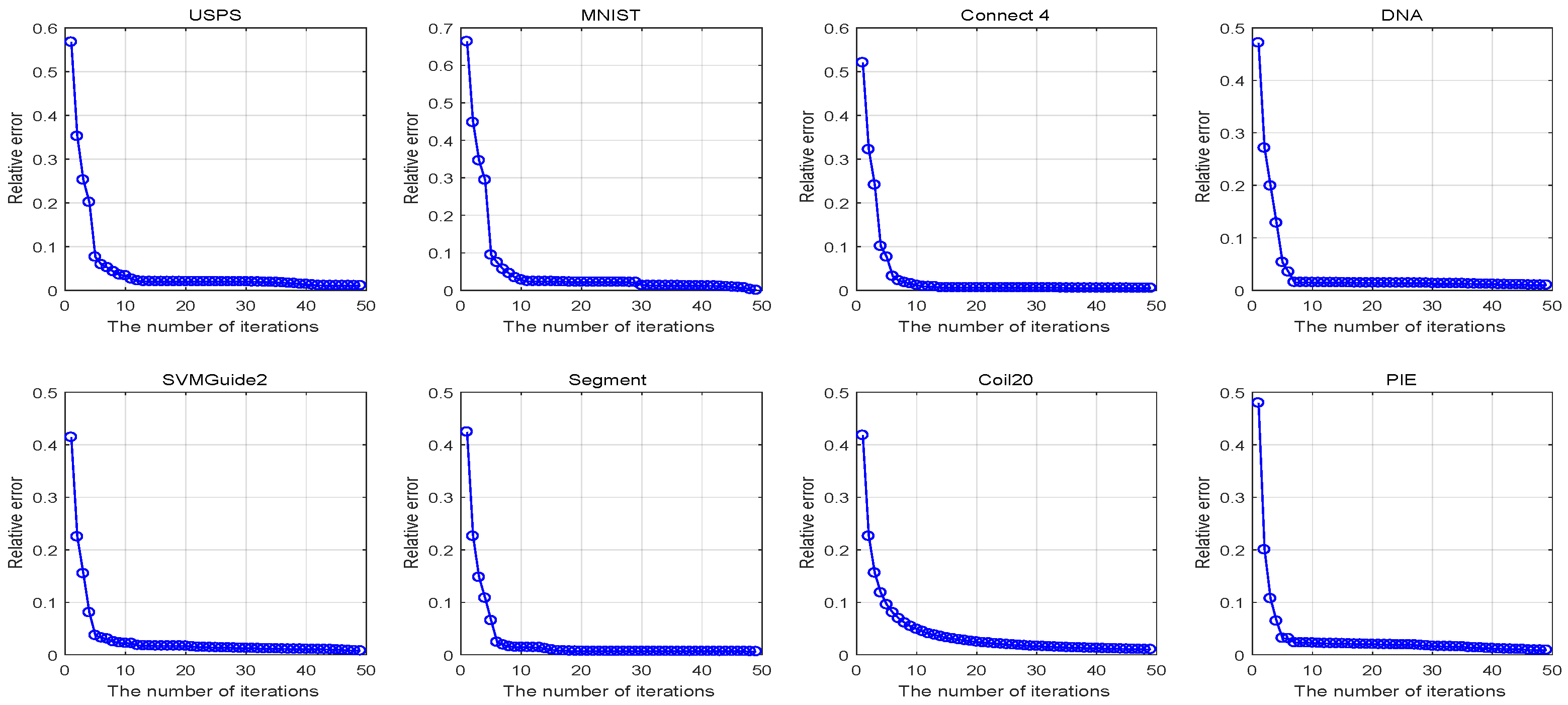
4.4. Convergence and Computational Performance

In this section, we provide the convergence curves of the proposed method over all the used datasets. Considering that the main focus of our discriminant analysis model is to learn the discriminative projection matrix $\mathbf{W}$, we directly use the relative error ${\displaystyle \frac{\parallel {\mathbf{W}}^{k+1}-{\mathbf{W}}^k{\parallel }_F}{\parallel {\mathbf{W}}^k{\parallel }_F}}\le {10}^{-4}$ as the convergence condition for Algorithm 1, where ${\mathbf{W}}^k$ denotes the value of $\mathbf{W}$ at the k-th iteration. Figure 6 shows the convergence curves of the relative error versus the number of iterations on different datasets. From Figure 6, we can see that our iterative optimization algorithm converges in less than ten iterations for most of the datasets, which indicates the efficiency of our iterative optimization algorithm.

To further investigate the computational performance of our method,

Table 6. Running time (seconds) of eight methods on eight benchmark datasets.

Dataset	LDA	MMC	NMMP	RFLD	RSLDA	MPDA	NLDA	LPMDA
USPS	0.213	0.387	1.675	0.721	1.369	2.912	2.163	0.392
MNIST	0.376	0.433	1.832	1.026	1.576	3.685	2.825	0.453
Connect4	1.368	1.830	6.122	4.651	5.216	12.377	6.933	1.836
DNA	1.231	1.682	5.331	3.685	4.921	11.937	6.387	1.721
SVMGuide2	0.086	0.122	0.468	0.329	0.453	0.975	0.637	0.151
Segment	0.131	0.173	0.621	0.467	0.526	1.265	0.861	0.210
Coil20	0.168	0.261	0.821	0.587	0.733	1.733	1.233	0.311
PIE	11.612	16.33	89.375	60.31	72.891	179.321	92.331	17.833

reports the training time of LPMDA and other related methods on the eight benchmark datasets. All experiments were set up as in the previous sections, and the results in Table 6 are the average training time over 20 repeated experiments. LDA has the shortest training time while MPDA has the longest training time. This is because MPDA requires computationally intensive matrix factorization operations. Our LPMDA runs slightly more slowly than LDA and MMC but achieves a marked improvement in discriminative performance. RFLD and RSLDA require an iterative solving of projection vectors, and NMMP and NLDA involve a complex computation of similarity graphs, and thus, both run slower than LPMDA.

4.5. Ablation Study

In LPMDA, the objective function contains two key schemes: geometric mean metric learning and auto-optimized graph embedding. To study the role each scheme plays in the dimension reduction problem, we conducted ablation experiments. The two degenerate versions of LPMDA are as follows:

• LPMDA1: LPMDA1 only replaces the trace ratio operation in LDA with the GMML similarity measure to obtain optimization problem (8), which can yield more features than the number of classes.
• LPMDA2: LPMDA2 incorporates auto-optimized graph embedding in LDA, resulting in the following optimization problem:

  $$\begin{array}{c}\hfill \underset{\mathbf{W},\mathbf{\Phi }}{max}{\displaystyle \frac{Tr\left({\mathbf{W}}^{\top }{\mathbf{S}}_b\mathbf{W}\right)}{Tr\left({\mathbf{W}}^{\top }{\tilde{\mathbf{S}}}_w\mathbf{W}\right)}},s.t.{\mathbf{\Phi }}_{j,:}^i\mathbf{1}=k,{\mathbf{\Phi }}_{j,h}^i\in \{0,1\}\end{array}$$

  (19)

where ${\mathbf{S}}_b$ is defined as (2), and ${\tilde{\mathbf{S}}}_w={\sum }_{i=1}^c{\sum }_{j=1}^{n_i}{\sum }_{h=1}^{n_i}{\displaystyle \frac{{\mathbf{\Phi }}_{j,h}^i}{n_i}}({\mathit{x}}_j^i-{\mathit{x}}_h^i){({\mathit{x}}_j^i-{\mathit{x}}_h^i)}^{\top }$.

Table 7. Results (%) (best average accuracy ± standard deviations%; optimal reduced dimensions) of the ablation study on benchmark datasets; the best results are highlighted in bold.

Dataset	USPS	MNIST	Connect 4	DNA	SVMGuide2	Segment	Coil20	PIE
LPMDA1	96.30 ± 0.92	87.03 ± 0.87	71.21 ± 1.12	82.11 ± 1.67	79.61 ± 1.22	88.63 ± 0.76	75.81 ± 1.26	92.36 ± 1.02
	(150)	(140)	(8)	(7)	(6)	(6)	(40)	(135)
LPMDA2	95.51 ± 2.33	85.61 ± 1.01	69.01 ± 1.21	80.38 ± 2.07	78.51 ± 0.91	89.26 ± 0.78	76.85 ± 0.98	91.48 ± 0.85
	(1)	(1)	(2)	(2)	(2)	(6)	(19)	(67)
LPMDA	98.89 ± 0.81	89.75 ± 0.85	74.21 ± 1.02	84.36 ± 1.71	81.37 ± 0.87	91.33 ± 0.69	77.23 ± 1.83	94.23 ± 0.72
	(150)	(140)	(6)	(4)	(4)	(6)	(35)	(120)

reports the ablation results of the proposed LPMDA on the eight benchmark datasets. From the table, it can be seen that LPMDA achieved the best performance on all datasets. For data with small class sizes, e.g., USPS MNIST, Connect 4, and DNA SVMGuide2, LPMDA 1 outperforms LPMDA 2. This is because LPMDA2 can extract much fewer features than LPMDA1, resulting in insufficient discriminative information. For Segment and Coil20, the number of features extracted by LPMDA2 is not significantly different from LPMDA1, but LPMDA2 embeds the additional local information, giving slightly better performance than LPMDA1. Therefore, we can conclude that both geometric mean metric learning and auto-optimized graph embedding can improve the performance of LPMDA.

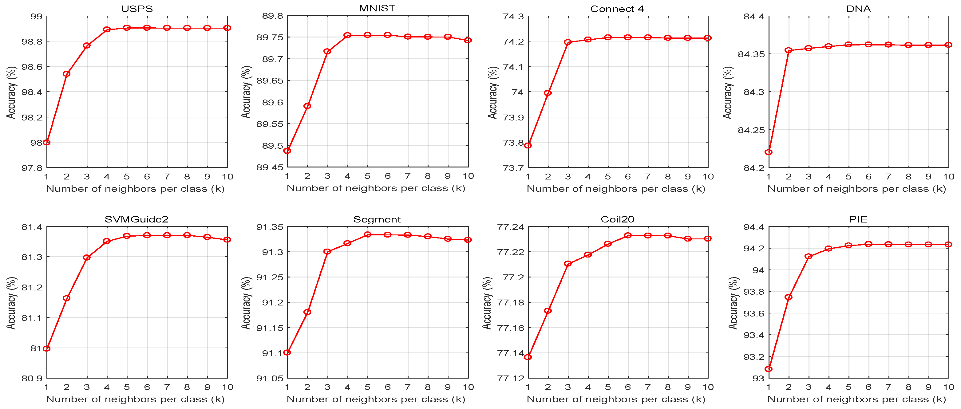
4.6. Parameter Sensitiveness

In order to obtain a more detailed view, we carried out experiments to see the effect of k on the performance of the proposed LPMDA. The accuracy varies with the number of neighbors per class (k), as shown in Figure 7. It can be seen that on these datasets, the performance of the LPMDA first improves and then stabilizes as k increases from 1 to 10. Furthermore, there is no significant difference in the performance of LPMDA on most datasets as k increases from 5 to 10. To balance the performance and efficiency, $k=5$ was set in the experiments.

5. Conclusions and Future Work

In this paper, we present a novel locality-preserving multiprojection discriminant analysis (LPMDA) framework that can directly extract enough discriminative features that preserve local structural information. Unlike the existing LDA-based methods, our proposed LPMDA maximizes the variance of the intraclass class while maximizing those of the interclass under the geometric mean metric learning framework, which can extract more features than the number of classes. Furthermore, an auto-optimized graph technique is introduced into the learning framework to fully exploit the local structure of the data from each class. More importantly, LPMDA has only one parameter to tune, making it very convenient to implement in real-world applications. Regarding the experiment, the odd–even digit recognition experiments on USPS and MNIST verified the effectiveness of LPMDA for data containing multiple clusters (or subclasses) within a class. The results and corresponding quantitative analysis in Table 4 indicate that LPMDA is significantly superior to other baselines, further validating its effectiveness in handling intraclass multimodal and small-class data. The experimental results on the six benchmark datasets in Figure 4 and the statistical significance results in Figure 5 further demonstrate the effectiveness of LPMDA in feature extraction for real data. The results in Table 6 indicate that the training time of LPMDA is slightly longer than that of LDA and MMC. However, all the computational costs associated with LPMDA only occur in the learning of the projection matrix. Once the features are extracted and ready for subsequent tasks, there will be no extra cost. In addition, the superior performance of LPMDA is sufficient to convince us that it is worth putting up with the computation overhead.

LPMDA provides a unified framework for feature extraction, and some more sophisticated metric learning or graph learning techniques can be easily plugged in to further extend it for some complex industrial big data. For example, introducing nonlinear metric learning or hypergraph learning techniques further enhances the model’s ability to handle nonlinear or class-overlapping data. The main computational complexity of LPMDA is focused on matrix operations, and the use of the instance selection technique to reduce its computational complexity is another major line of research.

References

1. Wang, J.; Wang, L.; Nie, F.; Li, X. Fast Unsupervised Projection for Large-Scale Data. IEEE Trans. Neural Netw. Learn. Syst. 2021, 33, 3634–3644. [Google Scholar] [CrossRef] [PubMed]
2. Dorrity, M.W.; Saunders, L.M.; Queitsch, C.; Fields, S.; Trapnell, C. Dimensionality reduction by UMAP to visualize physical and genetic interactions. Nat. Commun. 2020, 11, 1537. [Google Scholar] [CrossRef] [PubMed]
3. Yang, A.; Yu, W.; Zi, Y.; Chow, T. An Enhanced Trace Ratio Linear Discriminant Analysis for Fault Diagnosis: An Illustrated Example Using HDD Data. IEEE Trans. Instrum. Meas. 2019, 68, 4629–4639. [Google Scholar] [CrossRef]
4. Ma, J.; Xu, F.; Rong, X. Discriminative multi-label feature selection with adaptive graph diffusion. Pattern Recognit. 2024, 148, 110154. [Google Scholar] [CrossRef]
5. Yin, W.; Ma, Z.; Liu, Q. Discriminative subspace learning via optimization on Riemannian manifold. Pattern Recognit. 2023, 139, 109450. [Google Scholar] [CrossRef]
6. Xiang, C.; Fan, X.A.; Lee, T.H. Face Recognition Using Recursive Fisher Linear Discriminant. IEEE Trans. Image Process. 2006, 15, 2097–2105. [Google Scholar] [CrossRef]
7. Hemmatpour, S.; Hashemi, H. Using PCA and RDA feature reduction techniques for ranking seismic attributes. J. Earth Space Phys. 2011, 37, 217–227. [Google Scholar]
8. Fakhari, M.G.; Hashemi, H. Fisher Discriminant Analysis (FDA), a supervised feature reduction method in seismic object detection. Geopersia 2019, 9, 141–149. [Google Scholar]
9. Yan, S.; Xu, D.; Zhang, B.; Zhang, H.; Yang, Q.; Lin, S. Graph Embedding and Extensions: A General Framework for Dimensionality Reduction. IEEE Trans. Pattern Anal. Mach. Intell. 2007, 29, 40–51. [Google Scholar] [CrossRef]
10. Witten, D.M.; Tibshirani, R. Penalized Classification Using Fisher’s Linear Discriminant. J. R. Stat. Soc. Ser.-Stat. Methodol. 2011, 73, 753–772. [Google Scholar] [CrossRef]
11. Zhang, X.; Yang, T.; Long, H.; Shi, H.; Wang, J.; Yang, L. Fisher discrimination multiple kernel dictionary learning for robust identification of nonlinear features in machinery health monitoring. Inf. Sci. 2024, 677, 120862. [Google Scholar] [CrossRef]
12. Ju, F.; Sun, Y.; Gao, J.; Hu, Y.; Yin, B. Kronecker-decomposable robust probabilistic tensor discriminant analysis. Inf. Sci. 2021, 561, 196–210. [Google Scholar] [CrossRef]
13. Nie, F.; Wang, J.; Wang, H.; Li, X. Ratio Sum Versus Sum Ratio for Linear Discriminant Analysis. IEEE Trans. Pattern Anal. Mach. Intell. 1936, 44, 10171–10185. [Google Scholar]
14. Li, H.; Jiang, T.; Zhang, K. Efficient and robust feature extraction by maximum margin criterion. IEEE Trans. Neural Netw. Learn. Syst. 2006, 17, 157–165. [Google Scholar] [CrossRef]
15. Hayes, T.L.; Kanan, C. Lifelong Machine Learning with Deep Streaming Linear Discriminant Analysis. In Proceedings of the IEEE Conference on Computer Vision and Pattern Recognition Workshops, Seattle, WA, USA, 13–19 June 2020; pp. 887–896. [Google Scholar]
16. Bartan, B.; Pilanci, M. Neural Fisher Discriminant Analysis: Optimal Neural Network Embeddings in Polynomial Time. In Proceedings of the International Conference on Machine Learning, Baltimore, MD, USA, 17–23 July 2022; pp. 1647–1663. [Google Scholar]
17. Uzun, B.; Cevikalp, H.; Saribas, H. Deep Discriminative Feature Models (ddfms) for Set Based Face Recognition and Distance Metric Learning. IEEE Trans. Pattern Anal. Mach. Intell. 2023, 45, 5594–5608. [Google Scholar] [CrossRef] [PubMed]
18. Li, C.; Shao, Y.; Yin, W.; Liu, M. Robust and Sparse Linear Discriminant Analysis via an Alternating Direction Method of Multipliers. IEEE Trans. Neural Netw. Learn. Syst. 2020, 31, 915–926. [Google Scholar] [CrossRef]
19. Loog, M.; Ginneken, B.V.; Duin, R. Dimensionality reduction of image features using the canonical contextual correlation projection. Pattern Recognit. 2005, 38, 2409–2418. [Google Scholar] [CrossRef]
20. Zhu, M.; Martinez, A.M. Subclass Discriminant Analysis. IEEE Trans. Pattern Anal. Mach. Intell. 2006, 28, 1274–1286. [Google Scholar]
21. Webb, A.R. Introduction to Statistical Pattern Recognition. In Statistical Pattern Recognition; John Wiley & Sons: Hoboken, NJ, USA, 2003. [Google Scholar]
22. Sugiyama, M. Dimensionality reduction of multimodal labeled data by local fisher discriminant analysis. J. Mach. Learn. Res. 2007, 8, 1027–1061. [Google Scholar]
23. Li, Z.; Nie, F.; Chang, X.; Yi, Y. Beyond trace ratio: Weighted harmonic mean of trace ratios for multiclass discriminant analysis. IEEE Trans. Knowl. Data Eng. 2017, 29, 2100–2110. [Google Scholar] [CrossRef]
24. Wa, H.; Wang, H.; Guo, G.; Wei, X. Separability-Oriented Subclass Discriminant Analysis. IEEE Trans. Pattern Anal. Mach. Intell. 2018, 40, 409–422. [Google Scholar]
25. Luo, T.; Hou, C.; Nie, F.; Yi, D. Dimension reduction for non-gaussian data by adaptive discriminative analysis. IEEE Trans. Cybern. 2019, 49, 933–946. [Google Scholar] [CrossRef]
26. Okada, T.; Tomita, S. An optimal orthonormal system for discriminant analysis. Pattern Recognit. 1985, 18, 139–144. [Google Scholar] [CrossRef]
27. Ohta, R.; Ozawa, S. An Incremental Learning Algorithm of Recursive Fisher Linear Discriminant. In Proceedings of the International Joint Conference on Neural Networks, Atlanta, GA, USA, 14–19 June 2009; pp. 2310–2315. [Google Scholar]
28. Loog, M.; Duin, R. Linear Dimensionality Reduction via a Heteroscedastic Extension of LDA: The Chernoff Criterion. IEEE Trans. Pattern Anal. Mach. Intell. 2004, 26, 732–739. [Google Scholar]
29. Zadeh, P.; Hosseini, R.; Sra, S. Geometric mean metric learning. In Proceedings of the International Conference on Machine Learning, New York, NY, USA, 20–22 June 2016; pp. 2464–2471. [Google Scholar]
30. Fan, Z.; Xu, Y.; Zhang, D. Local Linear Discriminant Analysis Framework Using Sample Neighbors. IEEE Trans. Neural Netw. Learn. Syst. 2011, 22, 1119–1132. [Google Scholar] [CrossRef]
31. Nie, F.; Xiang, S.; Zhang, C. Neighborhood MinMax Projections. In Proceedings of the International Joint Conference on Artificial Intelligence, Hyderabad, India, 6–12 January 2007; pp. 993–998. [Google Scholar]
32. Zhao, Z.; Chow, T. Robust linearly optimized discriminant analysis. Neurocomputing 2012, 79, 140–157. [Google Scholar]
33. Zhu, F.; Gao, J.; Yang, J.; Ye, N. Neighborhood linear discriminant analysis. Pattern Recognit. 2022, 123, 108422. [Google Scholar] [CrossRef]
34. Zhou, Y.; Sun, S. Manifold Partition Discriminant Analysis. IEEE Trans. Cybern. 2017, 47, 830–840. [Google Scholar] [CrossRef]
35. Bhatia, R. Positive Definite Matrices. In Princeton; Princeton University Press: Princeton, NJ, USA, 2009; Volume 24. [Google Scholar]
36. Van der Maaten, L.; Hinton, G. Visualizing data using t-SNE. J. Mach. Learn. Res. 2008, 9, 2579–2605. [Google Scholar]
37. Sim, T.; Baker, S.; Bsat, M. The cmu pose, illumination, and expression database. IEEE Trans. Pattern Anal. Mach. Intell. 2003, 25, 1615–1618. [Google Scholar]
38. Demiar, J.; Schuurmans, D. Statistical Comparisons of Classifiers over Multiple Data Sets. J. Mach. Learn. Res. 2006, 7, 1–30. [Google Scholar]
39. Ma, J.; Zhou, S. Discriminative least squares regression for multiclass classification based on within-class scatter minimization. Appl. Intell. 2022, 52, 622–635. [Google Scholar] [CrossRef]
Figure 1. The overall framework of the proposed LPMDA. LPMDA aims to extract the low-dimensional discriminative features that preserve the local structure information between instances.
Mathematics 13 00962 g001
Figure 2. The digit samples in USPS and MNIST.
Mathematics 13 00962 g002
Figure 3. Visualization results of (a) T-SNE results of the original features; embedded features generated by (b) LDA, (c) NMMP, (d) MPDA, (e) NLDA, and (f) LPMDA. Note that all features are normalized to [−1,1].
Mathematics 13 00962 g003aMathematics 13 00962 g003b
Figure 4. Average accuracy with standard deviations (%) of seven baselines and our LPMDA on the six benchmark datasets. The red numbers below the x-axis denote the optimal reduced dimensions of different methods on the corresponding data.
Mathematics 13 00962 g004
Figure 5. CD diagram of different methods with significance level α = 0.05 .
Mathematics 13 00962 g005
Figure 6. Convergence curve of USPS, MNIST, Connect 4, DNA, SVMGuide2, Segment, Coil20, and PIE generated by LPMDA.
Mathematics 13 00962 g006
Figure 7. Accuracy varies with the number of neighbors per class (k) on the datasets.
Mathematics 13 00962 g007