Abstract
The main goal of this study is to develop a method for finding the joint probability distribution of the state of the characteristics of the NEMO (Nucleus for European Modeling of the Ocean) ocean dynamics model with data assimilation using the Generalized Kalman filter (GKF) method developed earlier by the authors. The method for finding the joint distribution is based on the Karhunen–Loeve decomposition of the covariance function of the joint characteristics of the ocean. Numerical calculations of the dynamics of ocean currents, surface and subsurface ocean temperatures, and water salinity were carried out, both with and without assimilation of observational data from the Argo project drifters. The joint probability distributions of temperature and salinity at individual points in the world ocean at different depths were obtained and analyzed. The Atlantic Meridional Overturning Circulation (AMOC) system was also simulated using the NEMO model with and without data assimilation, and these results were compared to each other and analyzed.
Keywords:
data analysis; Generalized Kalman filter (GKF); stochastic differential equations; data assimilation method; Karhunen–Loeve decomposition MSC:
60H30
1. Introduction
Data assimilation (DA) theory deals with the problem of correcting the numerical and (or) analytical model state in case the model numerical or analytical solution(s) do not coincide with the independently observed data. In particular, DA methods form one of the crucial directions of modeling in modern oceanography, meteorology, and climatology; they are widely applied in numerical weather forecasting and climate change studies. DA methods “optimally” combine the model output parameters and observations. Since, in general, the inverse problem for a nonlinear model has no solution and it is hard to find the initial condition for which the model trajectory coincides with the entire observational set, the DA problem may be formulated and solved only for particular cases. Apparently, on the one hand, there is no general solution of this problem; on the other hand, there are many approaches and methods that can be used to solve partially the DA problem for specific models and data sets.
Actually, in oceanography, DA theory is employed in conjunction with model simulation to construct and correct various model-produced characteristics in order to use them in a wide range of practical applications from oil and gas extraction to fishing and agriculture production. There are many oceanographic projects that apply DA methods to improve the prediction of ocean dynamics including the global projects GODAE [1,2], HYCOM–NCODA [3,4] and the regional projects BlueLink [5,6], REMO [7,8], TOPAZ [9] and several others.
Data assimilation methods have been developed for a long time—to be more exact, since the late 1960s. One of the first surveys on this area was presented in [10]. Later, DA methods were developed in [11,12,13] and many other papers.
In general, it is necessary not only to obtain the model output data and their variability after DA, but also to indicate their distribution or the distribution of errors, which appear after assimilation of a relatively “true” unknown state. If a stochastic dynamical scheme of DA is considered, this problem can be reformulated as the problem of finding the confidence bounds for the model output characteristics, provided that they are considered to be random. This is quite a difficult problem because of the nonlinearity of the stochastic process and the intrinsic dependence between the characteristics at different time instants. This is one of the problems solved in the current study.
Another problem in DA theory that had not been completely solved so far in its general statement is the physical understanding of how exactly does the assimilation process manifest itself in its physical aspects. In other words, it is interesting to know which spatial zones are more sensitive to data and how does the impact of DA vary in time and propagate in space. This problem is similar to the Fourier expansion for periodic analytical functions or to stationary stochastic processes. However, since the process under consideration is not stationary and the model fields are significantly anisotropic, this problem is not trivial. This is another subject of the current study.
This paper continues the studies published earlier in [14]. In those studies, the DA method called the Generalized Kalman filter (GKF) was used in application to ocean circulation models. The GKF method constructs a stochastic process which is optimal with respect to a given metric and satisfies a specific stochastic differential equation [14]. In the present study, the main attention is focused on the development of a method for finding the joint distribution of the random variables that correspond to the characteristics of the model during data assimilation. In addition, the GKF method is used in this work to simulate currents in the Atlantic describing the well-known AMOC phenomenon. Also, in Appendix A, a physical interpretation of the conditions of the theorems justifying the GKF method is given.
It is not sufficient to obtain only the model state after DA, it is necessary to find the confidence bounds of the determined variables. In other words, it is desirable and even necessary to calculate the probability distribution of the process under study provided that this process is assumed to be stochastic. One way to obtain the joint distribution of the state of the model characteristics after DA is to construct the corresponding Fokker-Planck-Kolmogorov equation (FPKE). However, solving the multidimension FPKE equation is a computationally complex problem.
Therefore, in this paper, another approach is proposed to find the joint distributions of the model characteristics. This approach is based on the Karhunen–Loeve decomposition of the covariance matrices [15,16]. With the use of this method, we find the desired joint distribution of the characteristics of the model. In [17], this method was tested on a one-day calculation using the Nucleus for European Modeling of the Ocean (NEMO) [18] and the GKF method.
The use of Karhunen–Loeve decomposition assumes consideration of dispersion-difference mixtures and finite difference autoregressions [19,20,21]. In the present work, we apply this technique to find the joint distributions.
2. The GKF Method of Data Assimilation
Let us briefly present the GKF method. This method is described in detail in [14]. We consider the following dynamical system:
where is the state-vector of the system, , and it is assumed that . The right-hand side of (1) is a non-linear vector-function.
The solution to (1) has the form
where is the initial condition. System (1) is considered in the probability space, since and are random vectors measurable with respect to the given probability measure P. At the same time, the vector-function is not random.
Let , be a discretization of the time interval and suppose that the DA method at a discrete time instant t has the form
where (the observed variable) is a random variable given in the same probability space which is independent of and measurable with respect to P; is the operator of projection of the state-vector onto ; and in general depends on ,, t. In the discrete approximation, X belongs to the space ; Y belongs to the space ; the weight matrix K has the size ; and the projective matrix H has the size . In time discretization for system (1) are taken at the same time instant .
In [14], it was established that as , the process defined by (2) converges weakly to the process X(t) which is the solution of the multi-dimensional stochastic differential equation
where , is the identity r × r matrix, is the r × r Wiener process with independent components, is the transpose of the matrix K, the matrix Q is defined by the limiting relation
and is the mathematical expectation with respect to the probability P. Mathematical conditions for the convergence with respect to Formulas (2) and (3), as well as the physical meaning of this convergence, are discussed in Appendix A.
In order for the DA problem to be solvable, the matrix should satisfy the condition of minimum of the matrix norm under the constraint , where is known from the observations. According to the GKF method [14], the optimal matrix K is as follows:
The denominator in (4) is a scalar.
Let be defined as
. In [22], it was shown that has the form
The corresponding Fokker–Planck–Kolmogorov equation has the form
Solving Equation (6) is very hard.
3. The Method of Decomposition of Covariances
The method for determining the key parameters of the GKF method, namely, the vector and the matrix , using the model output parameters and the data set at the time instant , as well as the previously calculated parameters and , is presented in detail, for instance, in [14] and [22], so we do not describe it here. As follows from (5), the matrix is determined uniquely as soon as and are known. The vector is defined by the formula , where, as was denoted above, x is the value of the process at the time instant (or t, if we consider the continuous case). The conditional mean value at the time step n + 1 can be found statistically as it was done in [14] and [22] for any model variable.
Below we present without proof two simple lemmas. Their proof and some comments can be found in [17].
Lemma 1.
If the model operator
is not a constant, in particular, if it is not zero, then the matrix has a full rank, it is positive definite and has a full set of eigenvectors and eigenvalues.
Lemma 2.
If the vector and the matrix are known, then the conditional probability of the variables is Gaussian distributed with the mean value and the covariance matrix .
These two lemmas imply the following theorem.
Theorem 1.
The increment of the vector variable ∆X is Gaussian distributed with the mean vector C and the covariance matrix
Proof.
Indeed, the increment can be represented as follows:
where are independent random Gaussian variables with zero mean and the covariance matrix for simplicity hereafter dependence on n is omitted. The representation (8) is derived with the use of the decomposition of matrix D, Formula (3) and the equality for a fixed t. Performing decomposition of the random variable with respect to the eigenvectors , we obtain from (3) the relation , where are expressed by the formula (scalar product) and are independent of each other. Since the Wiener process increment presents a Gaussian random variable with zero mean and the variance and are orthogonal and normalized, we obtain the assertion of Theorem 1.
We can continue our discussion. Hereafter, we use capital P to denote probabilities and lowercase p to denote densities.
Once the distribution of the increment is known, as it was found above at the time instant dt (or in the numerical realization, on the time interval ), the unconditional distribution of the process is defined by the formula
where is the Gaussian density
the covariance matrix is determined above in Formula (7). □
Therefore, we have established the following theorem.
Theorem 2.
The unconditional distribution of the random process (or in the discrete realization) that presents the model state after DA is defined by Formulas (9) and (10).
Corollary 1.
If the initial or restart distribution is given or statistically determined, then the distribution at step n can be found recurrently with the use of Formulas (9) and (10).
Corollary 2.
In the particular case, it follows from Formulas (9) and (10) that if
then
which means that is the Gaussian density.
Remark 1.
This numerical scheme of obtaining the probability distribution of the random process X(t) that represents the model state variable after DA at instant t is preferable in comparison with the calculation of the distribution by using Fokker–Planck–Kolmogorov Equation (6), especially if we deal with the multidimensional model state vector(s).
Remark 2.
Formula (9) allows for further generalizations. In particular, if the number n of steps is large enough (the asymptotic mode, n→∞) and there is a convergence of random variables, then Equation (9) transforms to the Fredholm integral equation, which can be solved analytically or numerically under some additional assumptions. However, this issue is out of the scope of the current study.
In conclusion of this section, let us prove the following theorem.
Theorem 3.
Suppose that the drift vector and the diffusion matrix are such that as t→∞ for all u except finitely many points, and is a positive definite continuous matrix, . Then, the sequence of probability measures satisfying the relation (9) has a limit as n goes to infinity.
Proof.
For the sake of brevity, we prove this theorem only in the one-dimensional case, the multivariate case is treated similarly. Additionally, we assume that the function is monotonically increasing and has a bounded second derivative for all Since this means that there are two moments or simply two natural numbers such as for any one can find two bounded functions that satisfy the equalities and This follows from the Taylor expansion and the boundedness of the second derivative of the function . Then, we can put these relations into (9) and obtain
where is the density of the standard Gaussian distribution. From this formula, after simple transformations, we obtain the relation
where the factor at is the average value of the corresponding integral. Since is continues and is not equaled everywhere to zero, the expression outside integral is small, has an order . On the other hand, functions , are bounded for all u and x and , for any m, n. Therefore, the expression (11) can be performed less for any and for large enough m, n. The Cauchy criterion is held, and Theorem 3 is proved. □
Remark 3.
The conditions when t→∞ have a clear physical sense. First condition means that the conditional mean (or ) in discrete realization when t goes tp infinity. This is a stationary condition. It means that asymptotically when the process reaches a level u then there are no changes of this process further in average. And the second condition simply means that the stochastic process (3) is not degenerated in time.
4. Numerical Experiments and Their Analysis
The GKF method with the NEMO model [18] has already been used earlier [23]. Numerical experiments were carried out with the NEMO model and with Argo database [24] on a high-performance computer K-60 [25] in the Keldysh Institute of Applied Mathematics of the Russian Academy of Sciences.
The ocean model NEMO in version 4.0.4 uses the computational grid ORCA025 with a horizontal resolution of around 0.25°. This grid includes 1442 × 1021 horizontal resolution and 75 vertical levels.
In the numerical experiments, we used the restart file [23]. The model was forced by the atmosphere data DRAKKAR [26]. The calculation process was launched on 5 August 2013; it lasted for one month and ended on 4 September 2013. Both the restart and atmosphere data were recorded on the same date; the Argo data were selected from the archive for the same month, and daily data assimilation was performed for each day according to Formulas (4) and (5), temperature, salinity and pressure data approximately from 3500 sea drifters ARGO were used daily. The diffusion matrix D and the drift vector C were as defined above.
Below, we present several figures that confirm the validity of the DA method and its capability to represent correctly the Atlantic Meridional Overturning Circulation (AMOC), as well as physical and numerical consequences of the model combined with the GKF method. Figure 1a,b show the AMOC dynamics for two different days corresponding to the beginning and the end of the experiment, namely, 5 August 2013, and 30 August 2013, respectively.
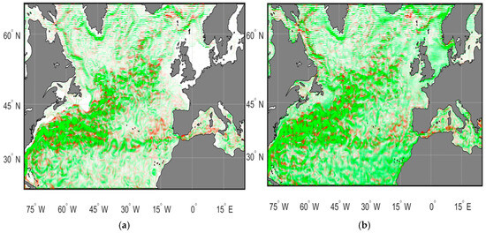
Figure 1.
Atlantic Meridional Overturning Circulation (AMOC) on two days: (a) 5 August 2013; (b) 30 August 2013. The green area marks current velocity (m/s) calculated by the model NEMO without data assimilation; the red area—with data assimilation.
Figure 1a,b clearly show that there is a good match of the GKF method and the NEMO model; however, this method intensifies the velocities of currents, especially in the Gulf Stream and equatorial current zones. In addition, the GKF method narrows the frontal zone and increases the gradient of model physical characteristics (not only velocities, but also temperature and salinity). Figure 1a,b also show that there is a pronounced temporal variability of the model currents with and without DA. One can see that the green area, as well as the red lines inside this area, become greater with time. This can be explained by intensification of dynamics due to data assimilation and atmosphere forcing present in the model.
The figures presented below demonstrate the spatial-temporal behavior of the eigenvectors and eigenvalues determined by the Formula (9). Figure 2a,b demonstrate the spatial behavior of the first eigenvector of temperature on the sea surface at two different time instants, namely, at the initial and final moments of integration, while Figure 2c,d show the spatial realization of the first eigenvector of temperature at the 100 m depth location at the same time instants.
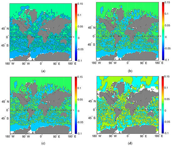
Figure 2.
Spatial behavior of the first eigenvector of temperature. At the sea-surface: (a) temperature increment on 5 August 2013; (b) temperature increment on 30 August 2013. At a depth of 100 m; (c) temperature increment on 5 August 2013; (d) temperature increment on 30 August 2013.
We can see that the structures of Figure 2a,b are somewhat similar; however, the temperature increment at the end of integration is weaker, since the colors are less saturated. It should be noted that the temperature increment is more pronounced along the Antarctic circumpolar current, in the equatorial zone and along the boundary currents, where strong upwelling effects occur. At a sea level of 100 m, the structure is much more chaotic; in general, the amplitude of increment is smaller. However, we can also see a weaker connection of the increment increase with the currents.
Figure 3a–d demonstrate the spatial and temporal behavior of salinity, which is similar to that of the temperature increment. Figure 3a,b show the first eigenvector of salinity at the sea surface; Figure 3c,d at a depth of 100 m.
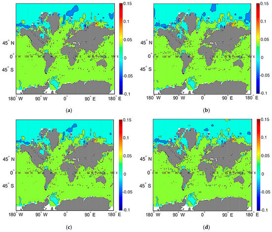
Figure 3.
Spatial behavior of the first eigenvector of salinity. At the sea surface: (a) salinity increment on 5 August 2013; (b) salinity increment on 30 August 2013. At a depth of 100 m; (c) salinity increment on 5 August 2013; (d) salinity increment on 30 August 2013.
Figure 3 shows that the first eigenvector of salinity has a weak dynamic. It should be noted that there are pronounced increments in the Weddell sea in the Antarctic zone, near the Amazonian Estuary, several spots in the Kuroshio current. In addition, it is possible to note several spots in the North Atlantic near Greenland and a positive red spot near the Taimyr Peninsula, namely, at the Faddey Bay in the East Siberian sea. There is no visible variability in time. As for the depth, one can see light-blue spots in the Arctic Ocean, more saturated blue spots in the Weddell sea, and also more pronounced blue spots near the Amazonian Estuary.
Let us note that Figure 2 and Figure 3 show the orthonormalized vectors that have a conditional rather than real physical meaning. To reduce those values to the real physical scale, it is necessary to multiply them by the eigenvalues according to Formula (9). In addition, their real physical values are obtained after multiplying the eigenvalues by the Gaussian random variable . The random vector is nonzero with a significant probability only in the small vicinity of the centers of ellipses. As a result, the expression has the same order as the average value .
Figure 4 shows the temporal behavior of eigenvalues. Since the first eigenvalue is much greater than the others, we can show only it on the same plane. It is seen that the first eigenvalue decreases during the first 5 days of integration and then remains relatively stable until the end of integration. Two other eigenvalues are by seven orders of magnitude smaller than the first one. For this reason, there is no sense to plot the second and third eigenvalues and the corresponding eigenvectors; their contributions to the resultant model state vector and its distribution are negligibly small.
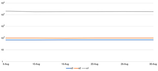
Figure 4.
Temporal behavior of eigenvalues over integration time. The gray curve refers to the first eigenvalue; the orange and blue curves, to the second and third eigenvalues, respectively.
Figure 5 shows the probability(is) of the joint distribution of the temperature and salinity increment (Gaussian random variable ) corresponding to the first eigenvector at three grid points with coordinates (0° N, 0° W), (0° N, 180° E), (46° N, 46° E) on the sea surface and at a depth of 100 m, respectively. These ellipses show three concentric lines of the levels corresponding to 0.3, 0.6 and 0.9 probabilities, respectively. In addition, these ellipses in Figure 5a–f show that there is a significant dependence between temperature and salinity (the correlation coefficient varies from 0.35 to 0.65), which strongly depends on the depth. And, finally, the ellipse at depth is larger than that on the sea surface, which is to say that the probability of having the same increment of temperature and salinity at depth is greater than that on the sea surface.
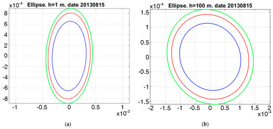
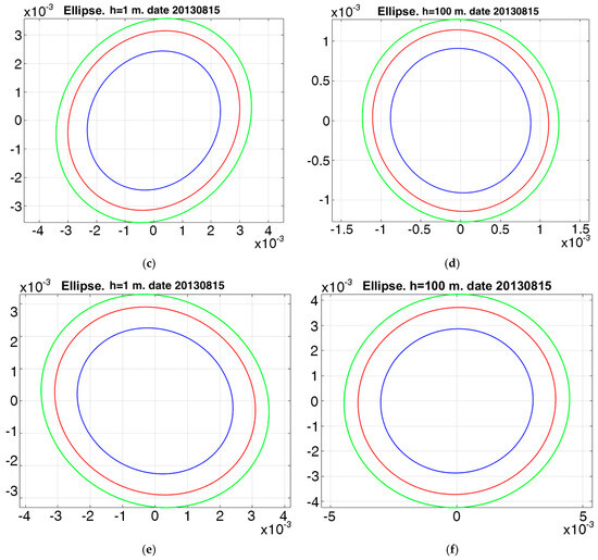
Figure 5.
Probability ellipses for the joint distribution of temperature and salinity for 15 August 2013 at the grid points with coordinates ((0° N, 0° W), (0° N, 180° E), (46° N, 46° E)) on the sea surface (a,c,e); at a depth of 100 m (b,d,f). Green, red and blue lines enclose the areas that correspond to the probability of 0.9, 0.6 and 0.3, respectively.
5. Conclusions and Outlook
In this study, a method for finding the joint probability distribution of the model variables in numerical experiments with data assimilation of observational data is proposed and theoretically substantiated. The new method for determining the joint distribution in general does not depend on a specific numerical model and dataset. The NEMO model and data from Argo drifters were used in this study because they were previously used by the authors in ocean modeling problems.
This problem has not been adequately considered in the scientific literature so far, since the process of its solving requires a rigorous analysis of random processes and their inner dependences, as well as a profound data analysis.
The calculation of the joint distribution by using recurrence formulas is feasible and computationally less costly than the calculation via the Fokker–Planck–Kolmogorov equation.
The joint probability distributions of such characteristics as temperature and salinity at individual points in the world ocean and at different depths were obtained. The maps of eigenvectors of covariance matrices, graphs for eigenvalues are presented, and scattering ellipses of these characteristics are constructed.
It has also been theoretically proven that as the assimilation process continues infinitely long, under certain restrictions imposed on the characteristics of the model, these characteristics exhibit a stationary Gaussian distribution. However, this is probably not the only possible mode and under different conditions it may appear to be quite different from Gaussian and may not exist at all. This problem will be the subject of our further study in the nearest future.
Also, calculations of the AMOC phenomenon in the Atlantic were also carried out with the use of the NEMO model with and without data assimilation.
Author Contributions
K.B. obtained theoretical results; A.K. carried out numerical experiments and analyzed their results; I.S. prepared observational data. All authors have read and agreed to the published version of the manuscript.
Funding
This work is supported by the Ministry of Science and High Education of Russian Federation, projects No. FMWE2024-0002-0016 (theoretical results, parts 2, 3, the first author) and No. FFMN-2025-0013 (numerical experiments, part 4, the second author).
Data Availability Statement
Data are contained within the article.
Conflicts of Interest
The authors declare no conflicts of interest. The founding sponsors had no role in the design of the study, in the collection, analysis or interpretation of data; in the writing of the manuscript, or in the decision to publish the results.
Appendix A. Mathematical Conditions of the Convergence of Sequences of Random Variables to a Stochastic Diffusion Process and Their Physical Interpretations
Let us consider the sequence of random variables (2).
All notations used in (2) are presented in Section 2, Formula (3) of the main body of this paper. All random variables are defined on the same probability space with the probability measure P.
Let the following conditions hold:
A1. , ,
A2. ,
A3..
Then, the sequence converges with respect to its distribution relatively P to the distribution of the random diffusion process satisfying Equation (3), where means the identity r-by-r matrix, and all other notations have been introduced above.
Let us discuss the physical meaning of the conditions A1–A3. The condition A1 means that the time interval between two consecutive assimilations is significantly smaller than the total integration time, T. Accordingly, the number of assimilation steps is large enough, . The product of these two variables t is moderate, its value lies between 0 and T and all the statements are valid at the time instant t.
The condition A2 means that the model is unbiased with respect to observations, if we know the model result at the time instant (the conditional average is zero). This condition is much weaker than the conventionally used condition of a priori unbiasedness, since we require only the time-dependent unbiasedness, posteriori, which means that the model can be “tuned” to observations while integrating, or on the contrary, the observations might be adapted to the model.
The condition A3 means that the conditional covariance (variance itself) grows in time as , i.e., at the same rate as the interval between consecutive assimilations. It is reasonable because if the interval between two consecutive assimilations is quite large, the variance (covariance) within the sample (assimilation window) is quite large as well. On the other hand, if the assimilation interval is small, the variance should also be small, the data are not “all lumped together”. All the conditions A1–A3 are physically reasonable and easily confirmed.
References
- Donton, C.; Robinson, I.; Casey, K.S.; Vazquez-Cuervo, J.; Armstrong, E.; Arino, O.; Gentemann, C.; May, D.; LeBorgne, P.; Piollé, J.; et al. The Global Ocean data assimilation experiment high-resolution Sea Surface Temperature Pilot Project. Bull. Am. Meteorol. Soc. 2007, 88, 1197–1214. [Google Scholar] [CrossRef]
- Powell, B.S.; Moore, A.M. Estimating the 4DVAR analysis error of GODAE products. Ocean Dyn. 2008, 59, 121–138. [Google Scholar] [CrossRef]
- HYCOM Consortium for Data Assimilative Modeling. Available online: http://www.hycom.org (accessed on 28 February 2025).
- Bleck, R. An oceanic general circulation model framed in hybrid isopycnic—Cartesian coordinates. Ocean Model. 2002, 4, 55–88. [Google Scholar] [CrossRef]
- Schiller, A.; Brassington, G.B.; Oke, P.; Cahill, M.; Divakaran, P.; Entel, M.; Freeman, J.; Griffin, D.; Herzfeld, M.; Hoeke, R.; et al. Bluelink ocean forecasting Australia: 15 years of operational ocean service delivery with societal, economic and environmental benefits. J. Oper. Oceanogr. 2020, 13, 1–18. [Google Scholar] [CrossRef]
- Chamberlain, M.A.; Oke, P.R.; Fiedler, R.A.S.; Beggs, H.M.; Brassington, G.B.; Divakaran, P. Next generation of Bluelink ocean reanalysis with multiscale data assimilation: BRAN2020. Earth Syst. Sci. Data 2021, 13, 5663–5688. [Google Scholar] [CrossRef]
- Mignac, D.; Tanajura, C.A.S.; Santana, A.N.; Lima, L.N.; Xie, J. Argo data assimilation into HYCOM with an EnOI method in the Atlantic Ocean. Ocean Sci. 2015, 11, 195–213. [Google Scholar] [CrossRef]
- Lima, L.N.; Pezzi, L.P.; Penny, S.G.; Tanajura, C.A.S. An investigation of ocean model uncertainties through ensemble forecast experiments in the Southwest Atlantic Ocean. J. Geophys. Res. Ocean. 2019, 124, 432–452. [Google Scholar] [CrossRef]
- Bertino, L.; Lisæter, K.A. The TOPAZ monitoring and prediction system for the Atlantic and Arctic Oceans. J. Oper. Oceanogr. 2008, 1, 15–18. [Google Scholar] [CrossRef]
- Ghil, M.; Malanotte-Rizzoli, P. Data assimilation in meteorology and oceanography. Adv. Geophys. 1991, 33, 141–266. [Google Scholar] [CrossRef]
- Zalesny, V.B.; Marchuk, G.I. Modeling of the world ocean circulation with the four-dimensional assimilation of temperature and salinity fields. Izv. Atmos. Ocean. Phys. 2012, 48, 15–29. [Google Scholar] [CrossRef]
- Evensen, G. The ensemble Kalman filter: Theoretical formulation and practical implementation. Ocean Dyn. 2003, 53, 343–367. [Google Scholar] [CrossRef]
- Xie, J.; Zhu, J. Ensemble optimal interpolation schemes for assimilating Argo profiles into a hybrid coordinate ocean model. Ocean Model. 2010, 33, 283–298. [Google Scholar] [CrossRef]
- Belyaev, K.; Kuleshov, A.; Tuchkova, N.; Tanajura, C.A.S. An optimal data assimilation method and its application to the numerical simulation of the ocean dynamics. Math. Comput. Model. Dyn. Systems 2018, 24, 12–25. [Google Scholar] [CrossRef]
- Karhunen, K. Über Lineare Methoden in der Wahrscheinlichkeitsrechnung; Annales Academiae Scientiarum Fennicae: Ser. A1; Kirjapaino oy. Sana: Helsinki, Finland, 1947. [Google Scholar]
- Loève, M. Probability Theory II. Graduate Texts in Mathematics, 4th ed.; Springer: Berlin/Heidelberg, Germany, 1978; Volume 46. [Google Scholar]
- Kuleshov, A.; Belyaev, K.; Smirnov, I.; Tuchkova, N. Statistical distribution of characteristics of the model solution after data assimilation. Lobachevskii J. Math. 2024, 45, 2328–2334. [Google Scholar] [CrossRef]
- Madec, G.; TheNEMO Team. NEMO Ocean Engine. Note du Polede Modélisation; del’Institut Pierre-Simon Laplace: Paris, France, 2016; Volume 27, Available online: https://www.nemo-ocean.eu/ (accessed on 7 February 2025).
- Nualart, D.; Pardoux, E. Boundary value problems for stochastic differential equations. Ann. Probab. 1991, 19, 1118–1144. [Google Scholar] [CrossRef]
- Ferrante, M.; Nualart, D. On the Markov property of a stochastic difference equation. Stoch. Process. Their Appl. 1995, 60, 131–146. [Google Scholar] [CrossRef][Green Version]
- Korolev, V.Y.; Chertok, A.V.; Korchagin, A.Y.; Zeifman, A.I. Modeling high-frequency order flow imbalance by functional limit theorems for two-sided risk processes. Appl. Math. Comput. 2015, 253, 224–241. [Google Scholar] [CrossRef][Green Version]
- Belyaev, K.P.; Kuleshov, A.A.; Tuchkova, N.P. Correction of systematic error and estimation of confidence limits for one data assimilation method. Lobachevskii J. Math. 2020, 41, 1964–1970. [Google Scholar] [CrossRef]
- Belyaev, K.P.; Kuleshov, A.A.; Resnyanskii, Y.D.; Smirnov, I.N.; Fadeev, R.Y. Numerical experiments with the NEMO ocean circulation model and the assimilation of observational data from Argo. Math. Mod. Comput. Simul. 2023, 15, 842–849. [Google Scholar] [CrossRef]
- Argo Data Sources. Available online: https://argo.ucsd.edu/data (accessed on 7 February 2025).
- Hybrid Computer K-60. Available online: http://www.kiam.ru/MVS/resourses/k60.html (accessed on 7 February 2025).
- Dussin, R.; Barnier, B.; Brodeau, L.; Molines, J.-M. DRAKKAR/MyOcean; Report 01-04-16; LGGE: Grenoble, France, 2016; Available online: https://www.drakkar-ocean.eu/publications/reports/report_DFS5v3_April2016.pdf (accessed on 7 February 2025).


Disclaimer/Publisher’s Note: The statements, opinions and data contained in all publications are solely those of the individual author(s) and contributor(s) and not of MDPI and/or the editor(s). MDPI and/or the editor(s) disclaim responsibility for any injury to people or property resulting from any ideas, methods, instructions or products referred to in the content. |
© 2025 by the authors. Licensee MDPI, Basel, Switzerland. This article is an open access article distributed under the terms and conditions of the Creative Commons Attribution (CC BY) license (https://creativecommons.org/licenses/by/4.0/).