Abstract
This paper takes as its starting point the distributed parameter models for both torsional and axial vibrations of the oilwell drillstring. While integrating several accepted features, the considered models are deduced following the Hamilton variational principle in the distributed parameter case. Then, these models are completed in order to take into account the elastic strain in driving signal transmission to the drillstring motions—rotational and axial (vertical). Stability and stabilization are tackled within the framework of the energy type Lyapunov functionals. From such “weak” Lyapunov functionals, only non-asymptotic Lyapunov stability can be obtained; therefore, asymptotic stability follows from the application of the Barbashin–Krasovskii–LaSalle invariance principle. This use of the invariance principle is carried out by associating a system of coupled delay differential and difference equations, recognized to be of neutral type. For this system of neutral type, the corresponding difference operator is strongly stable; hence, the Barbashin–Krasovskii–LaSalle principle can be applied. Note that this strong stability of the difference operator has been ensured by the aforementioned model completion with the elastic strain induced by the driving signals.
Keywords:
drillstring vibrations; Hamilton principle; distributed parameters; asymptotic stability; Lyapunov functionals; invariance principle MSC:
35L20; 34K20; 34K40; 93D30; 93D15
1. Introduction and Motivation
The problem of vibration quenching of the oilwell drillstring is extremely important from both technological and economic points of view. Here, the dedicated specialists provide telling insights. The oil extraction industry has existed for at least 150–200 years. Therefore, it is difficult to follow the entire literature pertaining to oil extraction, let alone the technology and the instrumentation developed. However, as pointed out in the preface of [1], “Vibrations in mechanical systems are oscillations occurring without being intentionally provoked. They often have detrimental effects on the system performance and may cause premature wear of the system components, underperforming processes, and could even involve security problems, such is the case in aircraft wings; which in the worst case scenario, excessive vibration causes the aircraft to crash. In oilwell drillstring systems, vibrations constitute an important source of economic losses; drill bit wear, pipes disconnection, borehole disruption and prolonged drilling time, are only some examples of consequences associated with drilling vibrations”. Continuing, this source further states, “Extensive research effort on the modeling and control of drilling systems has been conducted in the last century. Before the sixties, investigations were focused on material strength of the drillstring components, but the trends have since changed to emphasize on its dynamic behavior”. Nevertheless, the long list of references found in [1] —several hundred—contains only 3–4 sources that are older than 1965. One of them is [2], containing the first analytical and experimental study of torsional and axial drilling vibrations; in the list of references in [1] it is item [20].
In the last 2–3 decades, the distributed parameter drillstring dynamics was introduced. From the consulted literature (enumerated below), it appears that this is due less to limitations of the previous models or to computational difficulties than to the increased drilling depths requiring longer drillstrings. We encountered this description in [3], then the model was developed in [4], being afterwards adapted in the PhD thesis [5] and in subsequent papers [6,7,8]. In the same line, we can mention the surveys [9,10] and, with particular reference, the monograph [1]. More recently, we can mention the papers [11,12,13].
The aforementioned references deal with the distributed parameter drillstring dynamics and with the feedback control of vibration quenching. It is generally accepted that (nonlinear) vibrations are induced by the interaction of the rock-drilling bit, which is described by various nonlinear models [1,9,10]. On the other hand, other models of vibration ignition are available, taking into account the dynamics of the driving motors while considering a lumped parameter dynamics for the drillstring. We can cite here the PhD thesis [14] and the paper [15].
While the idea of discovering hidden oscillations of [15] looks interesting and very useful, we shall focus here on the first class of the aforementioned problems, i.e., vibration quenching for distributed parameter models. Our motivation is to emphasize the need for completing the model with the neglected terms, allowing us to obtain rigorous mathematical results for vibration quenching, considering both torsional and axial vibrations. As mentioned in [11], the torsional vibrations are most important for the drillstring. While the model structure allows us to consider the two types of vibrations separately, the mathematical aspects are slightly different.
The general scientific aim of the paper is the so-called augmented validation introduced in [16]. This means completing the standard validation representing well-posedness, as proposed by J. Hadamard (existence, uniqueness, continuity with respect to data—initial conditions and parameters—see, e.g., [17]) by adding stability properties. This extension results from the Stability Postulate of N. G. Četaev, a postulate which ascertains that only those motions (trajectories) can be “recognized” (measured, registered, observed) which are stable [18,19,20]. Turning to the usual approach of the Lyapunov function(al)s, we ascertain that the more adequate the model, the easier it is to find a “natural” Lyapunov function(al) and the closer to reality is the parameter stability domain.
In dynamical systems where energy is easy to describe, the energy Lyapunov function(al) appears as rather natural (e.g., in mechanical, electrical, or electromechanical systems). However, as the classic authors in stability theory have shown, the energy Lyapunov function(al) is a “weak” one, in the sense that its derivative along system trajectories is only non-positive; hence, asymptotic stability cannot be obtained directly from Lyapunov’s theorem on asymptotic stability—see, e.g., [21]—but rather from the Barbashin–Krasovskii–LaSalle invariance principle. Last but not least, the application of this principle would require pre-compactness of the bounded sets [22]. The stage of knowledge of this aspect for our models hints at the association of certain functional differential equations of neutral type. For such equations, it is known [22,23] that pre-compactness is ensured by the asymptotic stability of their difference operator. Throughout the paper, it will be apparent how this assumption is fulfilled due to the model improvements.
Therefore, the remaining sections of the paper are organized as follows. Firstly, the dynamics of both torsional and axial vibrations is presented, as resulting from the application of the Hamilton variational principle [24,25,26], and all basic notations are explained in Appendix A. Next, the steady states are defined and computed, and the deviations from the steady state are defined. The systems in deviations are mentioned and the energy-based Lyapunov functionals are associated thereto. The properties of the models and of the derivatives of the Lyapunov functionals allow us to obtain the uniform Lyapunov stability and global boundedness of the trajectories. These properties are obtained by synthesizing linear feedback controllers with dynamics, making use of the positiveness theory, i.e., the Yakubovich–Kalman–Popov lemma [27].
In order to obtain asymptotic stability by means of the Barbashin–Krasovskii–LaSalle invariance principle, systems of coupled delay differential and difference equations (recognized to be of neutral type [23] (p. 301)) are associated to the initial models described by partial differential equations of hyperbolic type with derivative boundary conditions. The solutions of the two mathematical objects are shown to be in one-to-one correspondence and, consequently, any mathematical result obtained for one of them is projected back on the other. Therefore, the asymptotic stability obtained for the systems of coupled delay differential and difference equations will give the same property for the initial models described by partial differential equations of hyperbolic type with derivative boundary conditions. Asymptotic stability results will be obtained first for each type of vibration model separately. However, the system of torsional vibrations introduces a perturbation in the system, modeling the axial vibrations. Consequently, the asymptotic stability is afterwards obtained for the coupled systems using a Lyapunov functional, which is a linear combination of those used for each system describing the drillstring vibrations (torsional and axial). The paper ends with conclusions and the enumeration of possible extensions of the obtained results.
2. The Model of the Coupled Torsional and Axial Vibrations of the Drillstring in Distributed Parameters
Practical experience shows that torsional vibrations are the dominant vibrations in drillstring dynamics. There are, however, a number of notable references displaying both types of vibrations coupled at the level of the drilling bit, with torsional vibrations acting on the axial ones, but without the reverse [1,9,10]. Here, we do not intend to compete with them, as our aim is to deduce both dynamics from the Hamilton variational principle. For a general explanation of this principle, the reader is sent to basic texts such as [24,28,29,30]. In the following, the Hamilton principle will be applied to mechanical systems subject to several external forces and torques. As will appear in the following, the “list” of the external forces and torques is of utmost importance in order to obtain an adequate mathematical model.
2.1. The Dynamics of Torsional Main Vibrations
Let us consider first the torsional main vibrations and construct the integral of the Hamilton principle. The rotational kinetic energy is given by
The potential energy due to the elastic strain is given by
Here and hereafter, we use . Obviously, we considered the general case of a space-inhomogeneous material, i.e., depending on —the linear coordinate along the drillstring—see Appendix A with paper-specific notations. Here, it has to be mentioned that, in all standard models reported in references—see again the long list of [1]—the material is considered homogeneous in space (the material parameters are constant). Our choice of non-constant parameters is not motivated by certain practical estimates of the non-homogeneities, but rather by the idea of obtaining the mathematical results within a framework as general as possible at the present level of knowledge.
The forms of the kinetic energy and elastic strain potential energy are standard, in fact quite well known; the reader is referred to [31,32,33,34]. From their form and structure, the choice of the generalized coordinates follows. As will be mentioned afterwards, the choice of the potential energy defines the type of the drillstring model (vibration string, Euler–Bernoulli, Kelvin–Voigt, Timoshenko).
The “list” of the generalized torques performing torsion and rotation, together with their expressions, is also given in Appendix A.
We write the work of the rotation torques
Consequently, the Hamiltonian of the rotational dynamics is defined by
where , are two arbitrary time moments.
2.2. The Dynamics of Axial Vibrations
Consider now the axial vibration dynamics. Define the kinetic energy
and the potential energy of the elastic strain by stretching and compression
As in the case of the torsional vibrations, here and hereafter, we use . The list of the generalized forces performing penetration and deformation work on the drillstring (along the vertical) is given in Appendix A.
We now write the work of the vertical forces as follows:
and the Hamiltonian of the axial dynamics
The Hamiltonian of the overall drillstring vibration dynamics will then be
2.3. The Perturbed Hamiltonians and the Euler–Lagrange Variations
Consider now the Euler–Lagrange variations of the generalized coordinates as follows:
where the bar variables account for a basic motion. Substituting (10) in the Hamiltonians, the perturbed Hamiltonians are obtained:
as follows:
and, analogously,
Formulae (12) and (13) show that is quadratic in both and ; however, the two “”-s never mix in the aforementioned expressions.
2.4. The Resulting Equations of the Dynamics
We shall recall now the Hamilton variational principle after [24], p. 113:
The motion of the mechanical system occurs in such a way that the definite integral (11) becomes stationary for arbitrary possible variations of the configuration of the system, provided the initial and final configurations are given.
The stationarity conditions of the integral are given by
It can also be seen from (12), (13) that the quadratic terms (in and ) are positive. Therefore, the Hessian matrix of is diagonal and positive definite. The stationary “point” defined by (14) is a minimum. Also, “prescribed initial and final configurations” means that all variations are 0 for , :
The two integrals and can be discussed separately, as (14) shows. Let us consider first the integral to find
After the application of the Fubini theorem and several integrations by parts, the following equations are obtained for any admissible motion:
The expressions of the torques, given in Appendix A, are also standard—lumped and distributed viscous friction torques and linear active torques, whose expressions are borrowed from standard textbooks on electromechanical drives and their control, e.g., [35]. The novelty here is that we took into account that application of the active torque implies both the rotation of the drillstring and the elastic torsional strain of it.
Substituting the various expressions for the torques in (16), the following boundary value problem is obtained:
This is a boundary value problem for a hyperbolic second-order partial differential equation. It is a non-standard boundary value problem since the boundary conditions contain derivatives and are coupled to certain ordinary differential equations. The partial differential equation represents the model of a vibrating string. This follows from the choice of the potential energy (2). Other equations, modeling Euler–Bernoulli, Kelvin–Voigt or Timoshenko beams, can be obtained by choosing the corresponding forms of the potential energy [31,32,36].
Let us consider now the integral , whose structure is analogous to that of . Again, the application of the Fubini theorem, integrations by parts and substitution of the various forces will give the following boundary value problem describing the dynamics of the axial vibrations:
Here, the same considerations on kinetic and potential energies as in the case of torsional vibrations and on acting friction and active force expressions are valid. A simple examination of (17) and (18) shows that the equations of (17) are quasi-linear because of the term , which is nonlinear; they contain the input (control) torque signal , which serves to control the torsional vibrations by a feedback control device. The torsional vibration dynamics is not affected by the axial dynamics and can be examined separately. The examination of (18) shows that the axial vibration dynamics system is linear, controlled by the input (control) force signal , but is also subject to an external perturbation signal arising from the torsional vibration dynamics. Consequently, the axial vibrations can also be analyzed separately, but taking into account the effect of the perturbation.
2.5. About the Nonlinear Load Torque at the Drilling Bit
To complete the discussion, we shall provide some details concerning the load torque at the drilling bit, as they can be found in the basic references. One of the simplest forms is given in [4]
This expression introduces a coupling between torsional and axial dynamics; the author substitutes with its steady state value, achieving the decoupling of the dynamics. In [1,9,10], the following expression is used, based on the models including Coulomb friction:
where . This expression contains a finite jump at :
Little is known about initial boundary value problems for hyperbolic partial differential equations with discontinuous right-hand side and, in order to achieve a rigorous mathematical treatment, discontinuous expressions for will be avoided. In previously cited references and surveys [1,9,10], the discontinuous models of —obtained from the use of various friction models (Coulomb, Karnopp)—were replaced by the following expression, considered to be a suitable approximation of the former:
In fact, as its graphical representation shows—Figure 1a—the approximation is mainly suitable around (the discontinuity point).
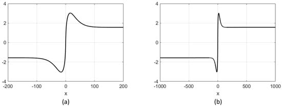
Figure 1.
Graphics of the rock–bit friction torque expressions: (a) rational approximation; (b) exparctan model.
Indeed, and also
The lower k is, the closer this approximation is to the discontinuity at (p is a scale factor, which adjusts the value of the extreme values). However, outside the interval , the slope of changes its sign (the graphic slowly approaches 0, asymptotically, for ) and can induce instabilities. The underlying idea is that, while is subject to a sector (Lurie-type) condition
the condition of the global Lipschitz type, that is,
which is necessary for the global asymptotic stability of an imposed steady state, is valid only on a bounded interval; consequently, asymptotic stability holds only on the bounded domains of the state space.
In [37,38], the following expression is used:
with . Some of its properties are mentioned below. Firstly, we observe that . Hence, is an odd function; its analysis for is sufficient, and it is enough to consider . Further,
Let us consider now the derivative
and ; hence, is increasing at least on a certain interval around . The zeros of follow from the equation
and, taking into account the values of given in [37,38], Equation (28) has two positive roots. As shown there, given by (26) appears as in Figure 1b, displaying a maximum and a minimum which are quite close, and then increasing very slowly up to . It follows that, by choosing, e.g., such that , the following will hold:
(after some elementary straightforward manipulation). In fact, (29) holds, provided that both , are not located where the slope of is negative. In practice, this condition is always fulfilled since the operating steady state point is defined by —the steady state angular speed—within the interval of the nonlinearity , corresponding to the maximal value of the nonlinear function . In the following, we shall refer to (26) for .
3. Cyclic Variables, Steady States and Energy Identity
3.1. The Cyclic Variables
A simple examination of (17) and (18) shows that , , , enter in these equations only by their time derivatives, i.e., they are cyclic variables; the equations provide information about the derivatives only while the angular and linear positions are irrelevant (the assertion obviously follows from physical considerations). We can therefore introduce the new variables
to obtain the models without the cyclic variables
and
3.2. The Steady States
The equations of the steady states of (31) and (32) are obtained by letting the time derivatives go to 0, thus obtaining
and
These two systems are also rather similar. We shall start the analysis with the system (33), obtaining firstly that . Next,
Therefore,
and is re-written as
that is, . We still have to examine
that is, two nonlinear equations with three unknown items. Usually, the angular velocity of the drillstring is imposed from technological considerations. Then, the system above becomes a linear one in the unknown items and , thus allowing us to obtain the steady state values for (31) from (33)
We turn now to (34), where is a known steady state forcing term “arising” from “outside” (the system of torsional vibrations). We have . Here also, the advancement (penetrating) linear velocity is imposed from technological considerations. Repeating the steps of the computation for the torsional vibration steady state, we obtain the steady state values for (32) from (34)
3.3. The Energy Identity
We shall now consider the energy identities for systems (31) and (32). We start with the system (31). We multiply the first partial differential equation by , the second one by , then add the two resulting equalities and integrate them with respect to s from 0 to L to obtain
In the same way, we obtain the energy identity for (32)
The next step is to take into account the boundary conditions of (31) by substituting and in (37) in order to obtain
The last term on the L(eft) H(and) S(ide) of the above identity is transformed as follows:
Summarizing, the following identity is obtained:
The same procedure is used for (38), taking into account the boundary conditions in (32)
The importance of the identities (39) and (40) will appear when applying the Lyapunov approach for controller synthesis and for proving asymptotic stability for the equilibrium describing the operating point of the drilling system.
4. The Systems in Deviations, Their Control and Stability
The problem which is tackled in this section is the design of the stabilizing feedback controller for torsional and axial dynamics, respectively, as well as the stability properties which are achieved this way.
4.1. Stability of the Controlled Torsional Vibrations Dynamics
Let us consider first the dynamics of the torsional vibrations (31) and its steady state (35). We shall first introduce the deviations from the steady state of the variables in (31)
where is given and , and are obtained from (35). The new variables satisfy the system in the deviations below:
Looking at (39), we can write immediately the analogous identity associated to (42)
Identity (43) suggests a feedback controller with its output containing . On the other hand, since the driving mechanism of the drillstring is located at ; the only possible input—technically speaking—is . We shall thus define the following linear controller:
under the following basic assumptions on it. It has inherent stability, i.e., is a Hurwitz matrix and the transfer function is an irreducible rational function; equivalently, is a controllable pair and is an observable pair.
In terms of feedback implementation, the choice of the controller (44) mainly means taking into account the dynamics of the elements composing the entire control subsystem. In our previous work, summarized in [16], the controller was modeled by a simple static (possibly nonlinear) expression with subject to a sector condition. It signified increasing the damping in the boundary dynamics at . The consideration of the controller dynamics provides various engineering solutions which can be found in [1] or in [11,13]. Our results deal with the mathematical aspects of pointing out the restrictions imposed on the controlling setup by the closed control loop stability conditions. These considerations also apply to the axial vibration controller.
Taking , i.e., a negative feedback connection, the identity (43) becomes
We are now able to define the following Lyapunov functional—written along the solutions of (42)–(44):
where is a symmetric matrix, which will be determined in the following. Differentiating and taking into account the identity (45), we obtain
The right-hand side of (47) contains obviously negative terms, including the term in ; see Figure 1b. We have to focus on the first three terms in (47)—the ones in and , also containing the symmetric matrix , whose choice and properties are yet to be determined. We turn to the Yakubovich–Kalman–Popov lemma [27,39], whose version, useful for our conditions, is given in Appendix B. In our case, and and the lemma reads as follows:
Assuming that the controller is such that (49) is valid, we take the symmetric matrix in (46) as the one prescribed by (48). Therefore, the derivative (47) of the Lyapunov functional (47) is at least non-positive.There is a symmetric matrix and a vector of appropriate dimensions such that the identityholds for any real vector and real scalar if and only if the following frequency domain inequalityholds for all frequencies .
In the following, we show that this will imply Lyapunov stability in the metrics induced by the Lyapunov functional itself of the zero equilibrium of the closed loop system in deviations, defined by (42) and (44). Therefore, we focus again on the matrix . From the Yakubovich–Kalman–Popov lemma, it is known that (48) holds for any reals and . Assume now that (48) holds, in particular, for some vector and scalar satisfying
even if they are not variables satisfying (42) and (44). As a more particular case, we shall assume and integrate (48) between 0 and t to obtain
and hence,
Since is a Hurwitz matrix, , , , thus resulting in a nonnegative definite, because is arbitrary with its initial condition. From and , we deduce that
On the other hand, let us consider components of a solution of (42) and (44). Since is a Hurwitz matrix, we have , , so that . Therefore, a straightforward manipulation will give
and (51) and (52) give the Lyapunov stability of the zero equilibrium of (42)–(44), as well as the global boundedness of the solutions. We have proven, in fact, that
Theorem 1.
Consider the closed loop controlled system (42) and (44) of the controlled torsional vibrations dynamics of the drillstring under the following assumptions: (i) is a Hurwitz matrix; (ii) the frequency domain inequality (49) holds; (iii) the nonlinearity defined by (26) satisfies
Then, the zero solution of (42) and (44) is Lyapunov stable in the metrics induced by the Lyapunov functional (46), a stability expressed by (51) and (52).
4.2. Stability of the Controlled Axial Vibration Dynamics
Let us consider now the dynamics of the axial vibrations. We shall proceed by analogy to the previous case of the torsional vibrations and point out the differences. Let us therefore consider the dynamics of the axial vibrations (32) and its steady state (36). Then, we shall introduce the deviations from the steady state of the variables in (32)
where is given and , and are obtained from (36). The new variables satisfy the system in the deviations below:
Looking at (40), we can write the analogous identity associated to (55):
The identity (56) suggests a feedback controller with its output containing —the deviation from the steady state. On the other hand, since the driving mechanism of the drillstring is located at , the only possible input—technologically speaking—is also . By analogy to the case of the torsional vibrations, we shall define the following linear controller:
under the same basic assumptions as in the previous case of the torsional vibrations. It has inherent stability, i.e., is a Hurwitz matrix and the transfer function is an irreducible rational function; equivalently, is a controllable pair and is an observable pair.
Now, a slight difference with respect to the previous case has to be taken into account; system (55) is subject to an external perturbation “arising” from the dynamics of the torsional vibrations and, as follows from Theorem 1, it is bounded for . From now on, we shall be interested in the inherent stability of (55) and will assume for a while that this external perturbation is identically zero.
We take —a negative feedback connection—and (56) becomes
(the perturbation term is now identically zero). We can now define the Lyapunov functional, written along the solutions of (55) and (57):
where is a symmetric matrix prescribed by the Yakubovich–Kalman–Popov lemma. Taking the derivative of combined with the identity (56)—without the perturbation generated term—it follows that
The last identity follows from the application of the Yakubovich–Kalman–Popov lemma under the positiveness frequency domain inequality
for all frequencies ; see (49) for comparison. From now on, the development follows the line of the previous, torsional vibration case. Based on the fact that is a Hurwitz matrix, we obtain that and, as in the previous case, Lyapunov stability is obtained in the sense of the metrics induced by the Lyapunov functional itself. Without reproducing the formulae which are analogous to (51) and (52), we provide the result below:
Theorem 2.
Consider the closed loop control system (55) and (57) of the controlled axial vibration dynamics under the following assumptions: (i) is a Hurwitz matrix; (ii) the frequency domain inequality (61) holds; (iii) the perturbation term is identically zero. Then, the zero solution of (55) and (57) is Lyapunov stable in the metrics induced by the Lyapunov functional (59).
5. Asymptotic Stability and Other Asymptotic Properties
The Lyapunov stability property has been obtained in the previous section by using the energy as Lyapunov functional. As is well known from publications by the classics of Lyapunov theory, such as N. G. Četaev, the energy Lyapunov function(al) is a “weak” one, which is easily constructed, but whose derivative along the system’s solutions is only non-positive (51) and (57); see, e.g., [40]. This fact, among others, led to the Barbashin–Krasovskii–LaSalle invariance principle, e.g., [21,41]. In the infinite dimensional case, however, its proof and application requires pre-compactness of the system’s bounded trajectories [22,42]—not easy to prove (notwithstanding, in the finite dimensional case, the bounded trajectories are also compact).
For this reason, we shall follow a path which goes back to Myshkis [43] and Cooke [44]. Our experience in this approach, summarized in [16], spans several decades. It consists of associating a system of functional differential equations—in most cases of neutral case—for which the Barbashin–Krasovskii–LaSalle invariance principle holds, to the basic system. Due to the one-to-one correspondence between the solutions of the two aforementioned mathematical objects (the initial-boundary value problem with derivative boundary conditions and the associated system of functional differential equations with deviated argument), the asymptotic stability obtained for one of them (the system of functional differential equations) is automatically projected back on the other. In the following, this approach will be applied to the dynamics of the drillstring vibrations.
5.1. Asymptotic Stability of the Equilibrium in the Torsional Vibration Case
We may call this aspect “asymptotic vibration quenching” in the torsional case. Consider the closed loop (with controller) system described by (42) and (44)—with —under the assumptions of zero distributed damping, i.e., and constant material parameters, i.e., , , . We shall thus have the following initial-boundary value problem with constant coefficients
We shall follow the procedure suggested in [44] and fully proven and described in [16]. Let us introduce firstly the Riemann invariants from
to associate to (62) the partial differential equations of the Riemann invariants
Substituting also (63) in the boundary conditions of (62), the transformed boundary conditions are associated to (64)
(We denoted ; the reason will appear in the following).
In the next step, we shall consider the two families of the characteristic straight lines—the solutions of
focusing on the two characteristics crossing some point . It is straightforward that the Riemann invariants are constant along the characteristics— along and along . Therefore, the following representation formulae are valid:
expressing the Riemann invariants as functions of their boundary values. Considering those characteristics which can be extended on the whole interval , we obtain the following relations between the boundary values of the Riemann invariants:
and they emphasize why is called the propagation time along the characteristics. Denoting
and substituting in (65), we obtain afterwards some straightforward manipulation
with the propagation time along the characteristics.
This system has the general form
and was introduced in our early papers [45,46] and recognized as reducible to a system of neutral type in [23], p. 301. Besides the development of the second author of this paper—see [16] for the state of the art—this system has recently received a renewed approach, e.g., [47]. The solution of (70) can be constructed by steps on intervals , (i.e., forward and backward), provided the initial ones are given on .
These initial conditions are obtained as follows: , , “migrate” from (62) to (70), while with are obtained by applying the following procedure. First, are obtained from and by taking the inverse of (63). Next, are obtained from the representation formulae (67); these formulae are considered now as being written along those characteristics which cannot be extended to the whole segment . Actually, each of them crosses the segment in some interior point . In fact, from the constance of the Riemann invariants along the characteristics, we shall have, based on (67), the following. From the first equality in (67), considering those characteristics crossing the abscissa , it follows that the crossing takes place at , . Therefore, ; hence, . In the same way, in the second equality of (67), we consider those characteristics crossing the abscissa at , . Further, we obtain . After a change of variables, we finally obtain
It appears that, considering a classical solution of (62) with some initial conditions , ,,,, we associated a solution of the system (70) of functional differential equations with the initial conditions with obtained from (71). The converse is also true. Consider a solution of (70), defined by some initial conditions with sufficiently smooth (e.g., continuously differentiable), then is a classical solution of (62), where migrate from the solution of (70) and are defined, as (67) and (69) suggest, by
and , follow from (63). The initial conditions of this solution follow by letting in the obtained expressions.
Summarizing, we have obtained the following result:
Theorem 3.
Consider a classical solution of (62) defined by some initial conditions , , , , , where we defined . Then, , , , is a solution of system (70), where are obtained via (63), (67), (69), with the initial conditions , , , , where are obtained from (71). Conversely, let us consider a solution of (70) defined by certain initial conditions , , , with sufficiently smooth, then , , , , is a classical solution of (62) with , defined from (72) and (63), the initial conditions being obtained by letting in the aforementioned solution of (62).
Now, Theorem 3 establishes a one-to-one correspondence between the solutions of two mathematical objects, i.e., (62) and (70), and any result regarding one of these objects is projected back on the other.
In particular, this will allow the application of the Barbashin–Krasovskii–LaSalle invariance principle to the system (70) in order to obtain asymptotic stability, which will afterwards migrate to (62). To do this, we shall associate to (70) a Lyapunov functional which is adapted from (46)—considered in the case of constant parameters. In fact, we have to express the integral in (46) using the representation formulae (72) and (63), recalling that and . The computations are quite straightforward and will give the following Lyapunov functional—written along the solutions of (70):
Differentiating it along the solutions of (70), we obtain, also based on the re-writing of (47), relying on the representation formulae (72):
This shows that the zero solution of (70) is Lyapunov stable in the sense of the metrics induced by the Lyapunov functional (73) itself. Based on Theorem 3, the Lyapunov stability in the sense of the Lyapunov functional (46) of system (42) and (44) is also obtained. However, this last result has been obtained directly in Section 4 in the more general case of the non-constant material parameters. But here, we shall also obtain asymptotic stability by applying the Barbashin–Krasovskii–LaSalle invariance principle for neutral functional differential equations, as stated in [23] (p. 293, Theorem 9.8.2).
First, we have to check that the condition in Theorem 9.8.2, concerning the asymptotic stability of the difference operator, is fulfilled. In the case of (70), this property is ensured by the location inside the unit disk of of the eigenvalues of the matrix
whose characteristic equation is
The property is true since . The Barbashin–Krasovskii–LaSalle invariance principle can thus be applied. In the set where vanishes, we have
It follows that in this set—the kernel of the derivative functional (74)—the dynamics of (70) is subject to the following system:
We deduce further that, in an invariant set included in the set defined by (76), ; hence, , , and hence, . It therefore follows from the differential equation of in (77) that , i.e., ; therefore, , following from the difference equations in (77). It remains to prove that . Now, since , , , it follows from the differential equation of in (77) that . Since is a controllable pair, is an observable pair. From the identity and from the observability, it follows that .
Consequently, the only invariant set included in the kernel of the derivative functional (74) is the equilibrium at 0. The application of the Barbashin–Krasovskii–LaSalle invariance principle will give, together with the already proven Lyapunov stability, the asymptotic stability of the zero equilibrium of the system of equations with deviated argument, as follows:
Based on the representation formulae (72) and on the definition of the Riemann invariants (63), it follows that
In fact, we obtained the asymptotic stability of the zero equilibrium of the system (62), of the system of its Riemann invariants (65) as well as of the system of functional differential equations with deviated argument (70). The results of Section 4 and of Section 5.1 can be summarized as follows:
Theorem 4.
Consider systems (62), (65) and (70) under the following basic assumptions: (i) all coefficients occurring in their equations are non-negative; (ii) the nonlinear function is subject to a global Lipschitz condition of (25) type; (iii) the controller (44) has inherent stability, i.e., matrix is a Hurwitz matrix and its transfer function is irreducible, i.e., is controllable and is observable; (iv) the transfer function satisfies the frequency domain inequality (49). Then, the zero equilibrium of the aforementioned systems is globally asymptotically stable.
5.2. Asymptotic Properties of the Axial Vibration Dynamics
5.2.1. The Autonomous System of the Axial Vibration Dynamics
Taking into account the similarities of the two kinds of dynamics, the exposition of the results in this subsection will be less extended than in the previous subsection. The assumptions on constant material parameters and zero distributed damping are valid here as well. Consequently, the basic closed loop system (i.e., with the synthesized controller) will result as follows:
To this system, we associate the Riemann invariants by
and the system written in the Riemann invariants
The two families of characteristic lines are solutions of the differential equations
Focusing on the two characteristics crossing some point , and taking into account that the Riemann invariants are constant along the characteristics— along and along —the following representation formulae are obtained:
giving the Riemann invariants as function of their boundary values. Considering those characteristics which can be extended on the whole interval , we obtain the following relations between the boundary values of the Riemann invariants
and appears as the propagation time along the characteristics. Denoting
and substituting in (82), the following system of coupled delay differential and difference equations is obtained:
The solution of (87) can be constructed in steps based on the initial conditions , where migrate from the initial conditions of (80) and , , are constructed starting from as follows:
Conversely, starting from a sufficiently smooth solution of (87), defining
and , from (81), then is a classical solution of (80). The mathematical result is similar to Theorem 3 and reads as follows:
Theorem 5.
Consider a classical solution of (80) defined by some initial conditions , , , , , where we defined . Then, , , , , where are defined via (81), (85) and (86), is a solution of the system of functional differential equations (87) with the initial conditions , , , , , being obtained from (88). Conversely, we shall consider a solution of (87) defined by certain initial conditions , , , , with sufficiently smooth (e.g., continuously differentiable). Then, , , , , is a classical solution of (80) with , defined from (89) and (81), the initial conditions resulting by letting in the aforementioned solution of (80). The forcing term is considered as given, defined by the system describing the dynamics of the torsional vibrations.
As in the case of Theorem 3, Theorem 5 establishes a one-to-one correspondence between the solutions of two mathematical objects, i.e., (80) and (87), and any result about one of these objects is projected back on the other. In particular, this will allow the application of the Barbashin–Krasovskii–LaSalle invariance principle to the system (87), in order to obtain asymptotic stability, which afterwards migrates to (80). Obviously, the stability properties will be obtained for the autonomous systems, i.e., by taking in (80) and (87).
We shall thus associate to (87) a Lyapunov functional, which is adapted from (59) in the case of constant parameters and by taking . Here, we also have to express the integral in (59) using the representation formulae (81), (84), (86) and recalling that , . The result will be
Differentiating it along the solutions of (87), we obtain, also based on the re-writing of (60):
The inequality (91) shows that the zero solution of the autonomous (without a forcing term) system (87) is Lyapunov stable in the sense of the metrics induced by the Lyapunov functional (90) itself. Based on Theorem 5, the Lyapunov stability in the metrics induced by the Lyapunov functional (59) for the system (80) is also obtained; this last result, however, was obtained directly in Section 4 in the most general case of non-constant material parameters. However, here we shall also obtain asymptotic stability by applying the Barbashin–Krasovskii–LaSalle invariance principle for neutral functional differential equations, as stated in [23] (p. 293, Theorem 9.8.2). Here also, as in the case of the torsional vibrations, we first have to check that the condition in Theorem 9.8.2, concerning the asymptotic stability of the difference operator, is fulfilled. In the case of system (87), this property is ensured by the location inside the unit disk of of the eigenvalues of the matrix
whose characteristic equation is
The property is true since . The Barbashin–Krasovskii–LaSalle invariance principle can thus be applied. In the set where vanishes, we have
It follows that, in this set—the kernel of the derivative functional (91)—the dynamics of (87) is subject to the following system:
We deduce further that, in an invariant set included in the set defined by (93), ; hence, , , and hence, . It therefore follows from the differential equation of in (94) that , i.e., ; therefore, , following from the difference equations in (94). It remains to prove that . Now, since , , , it follows from the differential equation of in (94) that . Since is a controllable pair, is an observable pair. Based on the identity and the observability, it follows that .
Consequently, the only invariant set included in the kernel of the derivative functional (91) is the equilibrium at 0. The application of the Barbashin–Krasovskii–LaSalle invariance principle will result, together with the already proven Lyapunov stability, in the asymptotic stability of the zero equilibrium of the autonomous system with deviated argument as follows:
Based on the representation formulae (89) and on the definition of the Riemann invariants (81), it follows that
In fact, we obtained the asymptotic stability of the zero equilibrium of the autonomous system (80), of the autonomous system (82) in the Riemann invariants as well as of the autonomous system (87) of functional differential equations with a deviated argument. The results from Section 4 and of Section 5.2 can be summarized as follows:
Theorem 6.
Consider the system (80) under the following basic assumptions: (i) all the coefficients occurring in its equations are non-negative; (ii) the forcing exogeneous signal is identically zero; (iii) the controller (57) has inherent stability, i.e., matrix is a Hurwitz matrix, its transfer function is also irreducible, i.e., is controllable and is observable; (iv) the transfer function satisfies the frequency domain inequality (61). Then, the zero equilibrium of the aforementioned systems (80), (82) and (87) is globally asymptotically stable.
5.2.2. The Perturbed System of the Axial Vibration Dynamics
After the stability analysis of the autonomous system (80) and of the associated systems (82) and (87), the behavior under the perturbation , which asymptotically approaches zero, still needs to be addressed. The asymptotics of the perturbed systems has been studied for a long time. We can refer the reader to such classical references as [21,41,48,49,50] dealing with stability with respect to persistent perturbations. Rather general and refined results on these topics can be found in the series of papers belonging to F. Brauer, A. Strauss and J. A. Yorke [51,52,53,54,55,56,57,58]. All aforementioned results deal with ordinary differential equations and strongly rely on the “good” properties of the associated Lyapunov functions.
Using these results here would probably require their extensions to functional differential equations or giving direct proofs based on the associated Lyapunov functionals. Fortunately, another approach, much simpler, is possible, since the perturbing signal in (80) originates from the system (62). These systems are connected in series; the signal is fed from (62) to (80), but there is no feedback between these systems. For these reasons, we shall consider the composite system (62) and (80) and the associated composite systems (65) and (82) of the Riemann invariants as well as the systems (70) and (87) of the functional differential equations with deviated arguments. Taking into account the one-to-one correspondence between their solutions, we shall start the stability analysis by focusing on the last composite system of functional differential equations, and associate the overall Lyapunov functional written along its solutions
where and are defined by (73) and (90), respectively; also, . Considering the derivative of (97) along the solutions of (70) and (87), we shall obtain
(see (74) and (91) for comparison). The novelty here is the pseudo-quadratic form
Taking into account the sector condition (25) or (29), provided the following inequality holds:
A rather elementary discussion, based on the second-degree trinomial properties, shows that, by choosing
the strict positiveness of is ensured provided (25) holds. Consequently, , and the stability of the composite system (70) and (87), in the metrics induced by the Lyapunov functional defined by (97), follows.
For the asymptotic stability, we shall turn again to the Barbashin–Krasovskii–LaSalle invariance principle. We shall first examine the asymptotic stability of the difference subsystem of the composite system; from (70) and (87), we can see that the two difference systems, which define asymptotically stable difference operators, do not interact. The characteristic equation of the difference operator is
and its roots are located on the vertical lines in
Next, the set where is defined in both (76) and (93). In this set—the kernel of the derivative function (98)—the equations of the composite system are defined by (77) and (94), which are decoupled. It follows from the previous development—performed for each of these systems separately—that the only invariant set contained in the kernel of the derivative function (98) is the equilibrium at the origin. Asymptotic stability follows from the equilibrium at 0 for (70) and (87). From the one-to-one correspondence between the solutions, the same property of the asymptotic stability for the equilibrium at the origin holds for the composite system of the Riemann invariants (65) and (82) as well as for the basic composite system of the vibration dynamics (62) and (80). These results are summarized in the following:
Theorem 7.
Consider the composite system of the coupled torsional and axial vibration dynamics of the drillstring defined by (62) and (80), together with the associate composite systems of the Riemann invariants (65) and (82) as well as of the coupled delay differential and difference Equations (70) and (87) under the assumptions of Theorems 4 and 6. Then, for each aforementioned system, the equilibrium at the origin is globally asymptotically stable.
Obviously, this theorem integrates the results of Theorems 4 and 6, strongly relying on Theorems 3 and 5.
Summarizing the mathematical development of the previous sections—with particular reference to the theorems on stability, i.e. Theorems 1, 2, 4, 6 and 7—it is important to re-affirm that the best validation of the mathematical results is their rigorous proofs. Computer simulations are intuitive and straightforward illustrations, adequate for practical uses, especially when the data are reliable, but neither validate nor strengthen a rigorous mathematical result. They were not envisaged for this research, but the interested reader can consult other research of ours [59,60,61]. Again, ref. [1], among others, contains more simulation results, which rely on existing mathematical models. Since our models are more developed and much more complicated, simulations based on the models of the present paper will be scheduled for a future work, and only then shall we be able to provide a reliable comparison with previous simulation results and models.
Another problem to be discussed here is connected with the (asymptotic) stability of the control loops of the drilling vibrations—namely, their performance or what is called quality of the transient process. In its turn, performance is connected to the selection of the controller parameters (the controller tuning). For linear (sub)systems, such as the unperturbed axial vibration control system, there are several ways of discussing quality: the convergence rate of the transient process (also called stability degree), error-integral criteria, frequency domain criteria (bounded peaking, stability margins) and others. They can be used in the selection of the controller parameters , , , —the coefficients of any of the two controllers considered in the paper. However, the controller is usually controllable and observable, i.e., its transfer function is irreducible and gives a complete description of the device which (a) is invariant to linear state transformations (coordinate change); (b) contains a minimal number of parameters.
The system of torsional vibrations is, however, nonlinear, and the methods of the linear systems do not apply. Here, the basic tool is again the Lyapunov function(al), which can be helpful, e.g., in stability convergence rate [21,62]. The convergence rate (stability degree) may be imposed, e.g., by considering a change of the state variables , where is the desired convergence rate, and , are the state vectors whose entries are any of the state variables of any of the considered systems. For the transformed system, the Lyapunov function(al) is associated; if this functional is quadratic (as it happens throughout the paper, since the energy function(al) is quadratic) and it does not increase along the system trajectories, then, along the starting system, we shall have , and this is nothing more than convergence in the norm induced by the Lyapunov functional itself with a guaranteed convergence rate (now of the exponential stability) α.
However, intuition suggests that cannot be chosen too large since the system cannot be forced (physically speaking) too far away from its “natural dynamics”. Even such “expensive” solutions as high gain, fast controller dynamics have limited possibilities; see the monographs on the performance limits of the control systems [63,64]. The other performance criteria mentioned above are mainly formulated for single linear control loops. Here, more than in the convergence rate, accurate knowledge of the performance limitations is crucial.
In our case, Theorems 4 and 6 contain such limiting indications—inclusive for the controllers. Indeed, the inherent stability of the controller together with the frequency domain inequalities (49) and (61) express the physical realizability conditions of E. A. Guillemin [65]. On the other hand, a realistic formulation of control quality is a specific engineering task and cannot be accomplished without the coordination of the triple “process engineer-control engineer-theoretician (applied mathematician or theoretically oriented engineer)”. Such a difficult task appears as “pending” if, for instance, one would consult again [1], where some 130 pages (a small/medium monograph) are dedicated to the control methods and controller structures for quenching drillstring vibrations as well as to control tuning. A careful lecture shows that, except for a general tackling of the convergence rate, most of the tuning procedures are oriented towards the fulfillment of stability conditions. Moreover, they are developed based on simplified models with lumped parameters; the delay models are exceptional in this third part of the monograph.
Turning once more to the use of the Lyapunov function(al)s, additional hints on their use, in obtaining transient performance by extending and adapting the methods of the linear systems, are given in [66]. The aforementioned Lyapunov function(al)s need to be “strong”, i.e., have strictly negative definite derivatives at least. This is not the case with the energy Lyapunov function(al) used throughout the paper, which, as already mentioned, is easily found, but “weak”.
Obviously, there is a lot to be done in this direction, falling outside the purposes and orientations of the present paper.
6. Conclusions and Prospective Research
The dynamics of the coupled torsional and axial vibrations of the drillstring was obtained in this paper by making use of the Hamilton variational principle. A careful listing of the acting forces and torques allowed the models in [16] to be completed, so that the resulting difference operators of the associated systems of functional differential equations with deviated argument are asymptotically stable. As a consequence, after obtaining uniform stability via the energy-like Lyapunov functional, it became possible to obtain asymptotic—even exponential—stability for the associated system of functional differential equations by applying the Barbashin–Krasovskii–LaSalle invariance principle. This property was then projected back on the initial system via the representation formulae for the Riemann invariants of the problem. The paper focused on the dynamics of the axial vibrations since this dynamics was forced by the coupling with the system of the torsional vibrations, the forcing signal asymptotically approaching zero, as a consequence of the asymptotic stability of the torsional vibration system. However, instead of using the results on the perturbed dynamical system from, e.g., [51,52,53,54,55,56,57,58], we considered the coupled torsional/axial vibration dynamics and a Lyapunov functional combined from those used separately. Once again, asymptotic stability was obtained by applying the Barbashin–Krasovskii–LaSalle invariance principle for the overall system.
From our point of view, the methodology applied in this paper is applicable to more complicated, but possibly more adequate, modeling—containing, e.g., nonlinear dependencies of the torques and forces on the state variables—as well as other models of the drillstring, viewed as a distributed parameter bar/beam/shaft [31,32]; the choice of the model depends on the choice of the elastic potential energy [36]. Moreover, the aforementioned aspects can be useful in the analysis of other mechanical systems.
Author Contributions
Formal analysis, V.R; investigation, D.D. and V.R; methodology, V.R.; supervision, V.R.; visualization, D.D. and V.R.; writing—original draft, D.D. and V.R.; writing—review and editing, D.D. and V.R. All authors have read and agreed to the published version of the manuscript.
Funding
This research received no external funding.
Data Availability Statement
The original contributions presented in the study are included in the article; further inquiries can be directed to the corresponding author.
Conflicts of Interest
The authors declare no conflicts of interest.
Appendix A. Notations
A. In the analysis of the torsional vibrations, the following notations are standard:
- —rotation angle of the driving mechanism, rotating the entire drillstring;
- —rotation angle of the drillstring at the cross-section and at ; this angle incorporates the torsion strain ;
- , —inertia moments of the driving system (located at ) and of the drilling bit (located at );
- —mass density of the drillstring at the cross-section ;
- —the polar momentum (geometric quantity) of the drillstring at the cross-section ;
- —the shear modulus of the drillstring at the cross-section .
Next, the list of the torques performing mechanical work of rotation and torsion is as follows:
- —the active driving torque supplied by the driving mechanism;
- —the damping torque at the shaft of the driving motor;
- —the torque applied by the driving motor to its load;
- —the load torque at the drillstring drive point (the torques , are virtual torques, occurring when separating the driving shaft from the drillstring at ; they might have equal absolute values if the drillstring were perfectly rigid—zero torsional strain);
- —the distributed damping torque due to the torsional friction; here, is the distributed friction coefficient of the drillstring at the cross-section ;
- —the damping torque at the drilling bit;
- —the load torque at the drilling bit; is a nonlinear, possibly discontinuous function.
B. In the analysis of the axial vibrations, the notations are as follows, most of them being standard:
- —vertical displacement of the drillstring, imposed by the brake motor of the driving mechanism;
- —vertical displacement of the drillstring at the cross-section and at , incorporating the strain ;
- —inertial mass of the vertical driving;
- —inertial mass of the drilling bit;
- —cross-isection area of the drillstring at the cross-section ;
- —elasticity Young modulus at .
The list of the generalized forces performing mechanical work of vertical displacement and axial strain is as follows:
- —the active force of vertical penetration supplied by the driving mechanism;
- —the damping force at the shaft of the driving mechanism;
- —the active force applied by the brake motor to its load;
- —the load force at the drillstring driving point (here, and are also virtual forces, occurring when separating the drive from the drillstring at ; they also might have equal absolute values if the drillstring were perfectly rigid—zero axial strain);
- —the distributed axial friction force, being the axial friction coefficient;
- —the damping force at the drilling bit;
- —the load rock/bit friction force, induced by the load friction torque at the bit;
- —the bit equivalent geometric radius;
- —conversion coefficient of the rotation friction into axial one;
- —friction coefficient.
As usual in mechanics, the dot over the variable denotes time derivative and subscripts s and t of the distributed variables denote partial derivatives.
Appendix B. The Yakubovich–Kalman–Popov Lemma
This result, which puts together properties from algebra and ordinary differential equations, stated and proven first by V. A. Yakubovich in 1962 [67] and in a different way by R. E, Kalman in 1963 [68], is now a special case of the general positivity theory due to V. M. Popov [27]. Throughout the paper, we use it in the very first form from 1962–1963, and it is under this form that we reproduce it below after [27] (p. 89).
Lemma A1.
Consider the pair where A is an matrix, b an n-vector and the triple , where κ is a real scalar, ℓ an n-vector and M an Hermitian matrix. Except κ, all other items have, generally speaking, complex entries. Define
where the asterisk denotes transpose and complex conjugation and . If is a controllable pair, then the frequency domain inequality
is necessary and sufficient for the existence of a scalar γ, an n-vector w and a Hermitian matrix N such that the following hold:
Moreover, if have real entries, then can be chosen with real entries.
References
- Saldivar, M.; Boussaada, I.; Mounier, H.; Niculescu, S.I. Analysis and Control of Oilwell Drilling Vibrations. A Time-Delay Systems Approach; Springer: Cham, Switzerland; New York, NY, USA; Heidelberg/Berlin, Germany, 2015. [Google Scholar]
- Bailey, J.J.; Finnie, I. An analytical study of drillstring vibration. J. Eng. Ind. Trans. ASME 1960, 82, 122–128. [Google Scholar] [CrossRef]
- Palmov, V.; Brommundt, E.; Belyaev, A. Stability analysis of drillstring rotation. Dyn. Stab. Syst. 1995, 10, 99–110. [Google Scholar] [CrossRef]
- Challamel, N. Rock destruction effect on the stability of a drilling structure. J. Sound Vib. 2000, 233, 235–254. [Google Scholar] [CrossRef]
- Saldivar, M. Analysis, Modeling and Control of an Oilwell Drilling System. Ph.D. Thesis, CINVESTAV Instituto Politecnico Nacional, Mexico City, Mexico, 2013. [Google Scholar]
- Saldivar, M.; Mondié, S.; Loiseau, J.; Rasvan, V. Stick-slip oscillations in oillwell drilstrings: Distributed parameter and neutral type retarded model approaches. IFAC Proc. Vol. 2011, 44, 284–289. [Google Scholar] [CrossRef]
- Saldivar, M.; Mondié, S.; Loiseau, J.; Rasvan, V. Exponential stability analysis of the drilling system described by a switched neutral type delay equation with nonlinear perturbations. In Proceedings of the 2011 50th IEEE Conference on Decision and Control and European Control Conference, Orlando, FL, USA, 12–15 December 2011; pp. 4164–4169. [Google Scholar]
- Saldivar, M.; Mondié, S.; Loiseau, J.; Rasvan, V. Suppressing axial-torsional coupled vibrations in drillstrings. J. Control Eng. Appl. Inform. 2013, 15, 3–10. [Google Scholar]
- Saldivar, M.; Boussaada, I.; Mounier, H.; Mondié, S.; Niculescu, S.I. An Overview on the Modeling of Oilwell Drilling Vibrations. IFAC Proc. Vol. 2014, 47, 5169–5174. [Google Scholar] [CrossRef]
- Saldivar, M.; Mondié, S.; Niculescu, S.I.; Mounier, H.; Boussaada, I. A control oriented guided tour in oilwell drilling vibration modeling. Annu. Rev. Control 2016, 42, 100–113. [Google Scholar] [CrossRef]
- Auriol, J.; Boussaada, I.; Shor, R.; Mounier, H.; Niculescu, S.I. Comparing Advanced Control Strategies to Eliminate Stick-Slip Oscillations in Drillstrings. IEEE Access 2022, 10, 10949–10969. [Google Scholar] [CrossRef]
- Ammari, K.; Beji, L. Spectral Analysis of the Infinite-Dimensional Sonic Drillstring Dynamics. Mathematics 2023, 11, 2426. [Google Scholar] [CrossRef]
- Faghihi, M.; Tashakori, S.; Yazdi, E.; Mohammadi, H.; Eghtesad, M.; van de Wouw, N. Control of Axial-Torsional Dynamics of a Distributed Drilling System. IEEE Trans. Contr. Technol. 2024, 32, 15–30. [Google Scholar] [CrossRef]
- Kiseleva, M. Oscillations and Stability of Drilling Systems: Analytical and Numerical Methods. Ph.D. Thesis, Sankt Petersburg State University, Saint Petersburg, Russia, 2013. [Google Scholar]
- Kiseleva, M.; Leonov, G.; Kuznetsov, N.V.; Neittaanmaki, P. Drilling Systems: Stability and Hidden Oscillations. In Discontinuity and Complexity in Nonlinear Physical Systems; Machado, J., Baleanu, D., Luo, A., Eds.; Number 6 in Nonlinear Systems and Complexity; Springer: New York, NY, USA; Heidelberg/Berlin, Germany, 2014; pp. 287–304. [Google Scholar]
- Răsvan, V. Augmented Validation and a Stabilization Approach for Systems with Propagation. In Systems Theory: Perspectives, Applications and Developments; Miranda, F., Ed.; Systems Science Series; Nova Publishers: New York, NY, USA, 2014; pp. 125–170. [Google Scholar]
- Courant, R. Hyperbolic partial differential equations. In Modern Mathematics for the Engineer: First Series; Beckenbach, E., Ed.; McGraw Hill: New York, NY, USA, 1956; pp. 92–109. [Google Scholar]
- Četaev, N. On the stable trajectories of the dynamics. Sci. Not. Kazan State Univ. 1931, 91, 3–8. (In Russian) [Google Scholar]
- Četaev, N. On the stable trajectories of the dynamics. Sci. Pap. Kazan Aviat. Inst. 1936, 4, 3–18. (In Russian) [Google Scholar]
- Răsvan, V. The stability postulate of N.G. Cetaev and the augmented model validation. IFAC-PapersOnLine 2017, 50, 7450–7455. [Google Scholar] [CrossRef]
- Barbashin, E.A. Lyapunov Functions; Physical & Mathematical Library of the Engineer, Nauka: Moscow, Russia, 1970. (In Russian) [Google Scholar]
- Saperstone, S. Semidynamical Systems in Infinite Dimensional Spaces; Applied Mathematical Sciences; Springer: New York, NY, USA; Heidelberg/Berlin, Germay, 1981; Volume 37. [Google Scholar]
- Hale, J.K.; Verduyn Lunel, S. Introduction to Functional Differential Equations; Number 99 in Applied Mathematical Sciences; Springer: New York, NY, USA, 1993. [Google Scholar]
- Lanczos, C. The Variational Principles of Mechanics, 4th ed.; Dover Publications, Inc.: New York, NY, USA, 1970. [Google Scholar]
- Akhiezer, N. Variational Calculus; Visča Škola: Kharkov, Russia, 1981. (In Russian) [Google Scholar]
- Gelfand, I.M.; Fomin, S.V. Calculus of Variations, 2nd ed.; Dover Publications, Inc.: New York, NY, USA, 1991. [Google Scholar]
- Popov, V.M. Hyperstability of Control Systems; Number 204 in Die Grundlehren der Mathematischen Wissenschaften; Springer: Berlin/Heidelberg, Germany; New York, NY, USA, 1973. [Google Scholar]
- Landau, L.; Lifshitz, E. Mechanics; Number 1 in Course in Theoretical Physics; Oxford University Press: Oxford, UK, 1976. [Google Scholar]
- Goldstein, H.; Poole, C.; Safko, J. Classical Mechanics, 9th ed.; Pearson: London, UK, 2013. [Google Scholar]
- Arnold, V. Mathematical Methods of Classical Mechanics; Springer: Berlin/Heidelberg, Germany; New York, NY, USA, 1989. [Google Scholar]
- Timoshenko, S.P.; Young, D.H.; Weaver, W. Vibration Problems in Engineering; John Wiley & Sons: New York, NY, USA; London, UK; Sydney, Australia; Toronto, ON, Canada, 1974. [Google Scholar]
- Meirovitch, L. Analytical Methods in Vibrations; Macmillan: New York, NY, USA; London, UK, 1974. [Google Scholar]
- Meirovitch, L. Elements of Vibration Analysis; McGraw-Hill: New York, NY, USA; Toronto, ON, Canada; London, UK, 1975. [Google Scholar]
- Den Hartog, J.P. Mechanical Vibrations; Dover Publications: New York, NY, USA, 1985. [Google Scholar]
- Leonhard, W. Control of Electrical Drives; Power Systems; Springer: Berlin/Heidelberg, Germany; New York, NY, USA, 2001. [Google Scholar]
- Russell, D. Mathematical models for the elastic beam and their control-theoretic implications. In Proceedings of the Semigroups, Theory and Applications (Proceedings Trieste, 1984) vol.II; Brézis, H., Crandall, M., Kappel, F., Eds.; Number 152 in Pitman Research Notes in Mathematics; Longman Scientific and Technical: New York, NY, USA, 1986; pp. 177–216. [Google Scholar]
- Li, L.; Zhang, Q.; Rasol, N. Time-Varying Sliding Mode Adaptive Control for Rotary Drilling System. J. Comput. 2011, 6, 564–570. [Google Scholar] [CrossRef]
- Bresch-Pietri, D.; Krstic, M. Adaptive output feedback for oil drilling stick-slip instability modeled by wave PDE with anti-damped dynamic boundary. In Proceedings of the 2014 American Control Conference, Portland, OR, USA, 4–6 June 2014; pp. 386–391. [Google Scholar]
- Halanay, A.; Rasvan, V. Applications of Liapunov Methods in Stability; Mathematics and Its Applications; Kluwer Academic Publishers: Dordrecht, The Netherlands, 2012; Volume 245. [Google Scholar]
- Rouche, N.; Habets, P.; Laloy, M. Stability Theory by Liapunov’s Direct Method; Applied Mathematical Sciences; Springer: Berlin/Heidelberg, Germany; New York, NY, USA, 1977; Volume 22. [Google Scholar]
- LaSalle, J.P.; Lefschetz, S. Stability by Lyapunov’s Direct Method with Applications; Mathematics in Science and Engineering; Academic Press: New York, NY, USA; London, UK, 1961; Volume 4. [Google Scholar]
- Haraux, A. Systèmes Dynamiques Dissipatifs et Applications; Recherches en Mathématiques Appliquées; Masson: Paris, France; Milan, Italy; Barcelone, Spain, 1991; Volume 17. [Google Scholar]
- Abolinia, V.; Myshkis, A. Mixed problem for an almost linear hyperbolic system in the plane (Russian). Mat. Sbornik 1960, 50, 423–442. [Google Scholar]
- Cooke, K.L. A linear mixed problem with derivative boundary conditions. In Seminar on Differential Equations and Dynamical Systems (III); Sweet, D., Yorke, J., Eds.; Lecture Series; University of Maryland: College Park, MD, USA, 1970; Volume 51, pp. 11–17. [Google Scholar]
- Răsvan, V. Absolute stability of a class of control systems described by coupled delay-differential and difference equations. Rev. Roum. Sci. Techn. Sér. Electrotechn. Energy 1973, 18, 329–346. [Google Scholar]
- Răsvan, V. Absolute stability of a class of control processes described by functional differential equations of neutral type. In Equations Differentielles et Fonctionelles Nonlineaires; Janssens, P., Mawhin, J., Rouche, N., Eds.; Hermann: Paris, France, 1973; pp. 381–396. [Google Scholar]
- Gu, K.; Huan, P.V. External Direct Sum Invariant Subspace and Decomposition of Coupled Differential-Difference Equations. IEEE Trans. Autom. Control 2024, 69, 1022–1028. [Google Scholar] [CrossRef]
- Malkin, I.G. Theory of Stability of Motion: Translated from a Publication of the State Publishing House of Technical-Theoretical Literature, Moscow-Leningrad, 1952; US Atomic Energy Commission, Office of Technical Information: Kansas City, MO, USA, 1959; Volume 3352. [Google Scholar]
- Yoshizawa, T. Stability Theory by Liapunov’s Second Method; Publications of the Mathematical Society of Japan; The Mathematical Society of Japan: Tokyo, Japan, 1966; Volume 9. [Google Scholar]
- Halanay, A. Differential Equations. Stability. Oscillations. Time Lags; Mathematics in Science and Engineering; Academic Press: New York, NY, USA; London, UK, 1966; Volume 23. [Google Scholar]
- Brauer, F. Perturbations of Nonlinear Systems of Differential Equations I. J. Math. Anal. Appl. 1966, 14, 198–206. [Google Scholar] [CrossRef]
- Brauer, F. Perturbations of Nonlinear Systems of Differential Equations II. J. Math. Anal. Appl. 1967, 17, 418–434. [Google Scholar] [CrossRef]
- Brauer, F. Perturbations of Nonlinear Systems of Differential Equations III. J. Math. Anal. Appl. 1970, 31, 37–48. [Google Scholar] [CrossRef]
- Brauer, F. Perturbations of Nonlinear Systems of Differential Equations IV. J. Math. Anal. Appl. 1972, 37, 214–222. [Google Scholar] [CrossRef]
- Strauss, A.; Yorke, J.A. Perturbation Theorems for Ordinary Differential Equations. J. Differ. Equ. 1967, 3, 15–30. [Google Scholar] [CrossRef]
- Strauss, A.; Yorke, J.A. Perturbing asymptotically stable differential equations. Bull. Am. Math. Soc. 1968, 74, 992–996. [Google Scholar] [CrossRef]
- Strauss, A.; Yorke, J.A. Identifying perturbations which preserve asymptotic stability. Proc. Am. Math. Soc. 1969, 22, 513–518. [Google Scholar] [CrossRef]
- Strauss, A.; Yorke, J.A. Perturbing Uniform Asymptotically Stable Nonlinear Systems. J. Differ. Equ. 1969, 6, 452–483. [Google Scholar] [CrossRef]
- Danciu, D. Numerics for hyperbolic partial differential equations (PDE) via Cellular Neural Networks (CNN). In Proceedings of the 2nd International Conference on Systems and Computer Science Conference, Villeneuve d’Ascq, France, 26–27 August 2013; pp. 183–188. [Google Scholar]
- Danciu, D.; Boussaada, I.; Stîngă, F. Computational modeling and oscillations damping of axial vibrations in a drilling system. In Proceedings of the 2018 22nd International Conference on System Theory, Control and Computing (ICSTCC), Sinaia, Romania, 10–12 October 2018; pp. 105–110. [Google Scholar]
- Stîngă, F.; Danciu, D. A Disturbance Observer-Based Control of Drilling Vibrations. In Proceedings of the 2019 20th International Carpathian Control Conference (ICCC), Kraków, Poland, 26–29 May 2019; pp. 1–6. [Google Scholar]
- Barbashin, E.A. Introduction to Stability Theory; Physical & Mathematical Library of the Engineer, Nauka: Moscow, Russia, 1967. (In Russian) [Google Scholar]
- Boyd, S.P.; Barratt, C.H. Linear Controller Design: Limits of Performance; Cliffs, N.J., Ed.; Prentice-Hall Information and System Sciences; Prentice Hall: Englewood, CO, USA, 1991; Volume 78. [Google Scholar]
- Seron, M.M.; Braslavsky, J.H.; Goodwin, G.C. Fundamental Limitations in Filtering and Control; Communications and Control Engineering; Springer: Berlin/Heidelberg, Germany; New York, NY, USA, 1997. [Google Scholar]
- Guillemin, E.A. Synthesis of Passive Networks; John Wiley & Sons: New York, NY, USA, 1957. [Google Scholar]
- Helton, J.W.; James, M.R. Extending H∞ Control to Nonlinear Systems. Control of Nonlinear Systems to Achieve Performance Objectives; Advances in Design and Control; SIAM: Philadelphia, PA, USA, 1999. [Google Scholar]
- Yakubovich, V.A. Solution of Some Matrix Inequalities Met in Automatic Control Theory. Dokl. Akad. Nauk SSSR 1962, 143, 1304–1307. (In Russian) [Google Scholar]
- Kalman, R.E. Lyapunov functions for the problem of Lur’e in automatic control. Proc. Natl. Acad. Sci. USA 1963, 49, 201–205. [Google Scholar] [CrossRef]
Disclaimer/Publisher’s Note: The statements, opinions and data contained in all publications are solely those of the individual author(s) and contributor(s) and not of MDPI and/or the editor(s). MDPI and/or the editor(s) disclaim responsibility for any injury to people or property resulting from any ideas, methods, instructions or products referred to in the content. |
© 2025 by the authors. Licensee MDPI, Basel, Switzerland. This article is an open access article distributed under the terms and conditions of the Creative Commons Attribution (CC BY) license (https://creativecommons.org/licenses/by/4.0/).