Large Language Model-Guided SARSA Algorithm for Dynamic Task Scheduling in Cloud Computing

Abstract

Nowadays, more enterprises are rapidly transitioning to cloud computing as it has become an ideal platform to perform the development and deployment of software systems. Because of its growing popularity, around ninety percent of enterprise applications rely on cloud computing solutions. The inherent dynamic and uncertain nature of cloud computing makes it difficult to accurately measure the exact state of a system at any given point in time. Potential challenges arise with respect to task scheduling, load balancing, resource allocation, governance, compliance, migration, data loss, and lack of resources. Among all challenges, task scheduling is one of the main problems as it reduces system performance due to improper utilization of resources. State Action Reward Action (SARSA) learning, a policy variant of Q learning, which learns the value function based on the current policy action, has been utilized in task scheduling. But it lacks the ability to provide better heuristics for state and action pairs, resulting in biased solutions in a highly dynamic and uncertain computing environment like cloud. In this paper, the SARSA learning ability is enriched by the guidance of the Large Language Model (LLM), which uses LLM heuristics to formulate the optimal Q function. This integration of the LLM and SARSA for task scheduling provides better sampling efficiency and also reduces the bias in task allocation. The heuristic value generated by the LLM is capable of mitigating the performance bias and also ensuring the model is not susceptible to hallucination. This paper provides the mathematical modeling of the proposed LLM_SARSA for performance in terms of the rate of convergence, reward shaping, heuristic values, under-/overestimation on non-optimal actions, sampling efficiency, and unbiased performance. The implementation of the LLM_SARSA is carried out using the CloudSim express open-source simulator by considering the Google cloud dataset composed of eight different types of clusters. The performance is compared with recent techniques like reinforcement learning, optimization strategy, and metaheuristic strategy. The LLM_SARSA outperforms the existing works with respect to the makespan time, degree of imbalance, cost, and resource utilization. The experimental results validate the inference of mathematical modeling in terms of the convergence rate and better estimation of the heuristic value to optimize the value function of the SARSA learning algorithm.

1. Introduction

Modern enterprises are shifting towards cloud computing as it provides flexibility and ubiquitous access to services, leading to better customer satisfaction. It is a strategic decision to mitigate the risks of higher cost of operation and delay in service delivery. Cloud-adapted enterprises benefit from more resilience and greater agility by integrating DevOps practices with traditional software development. Some of the challenges associated with cloud computing are service quality, portability, limited resources, adaptability, compliance, task scheduling, workload fluctuation, and resource failures [1,2]. Task scheduling plays an important role in enhancing the performance of cloud services by the proper utilization of the resources in terms of processor, memory, and bandwidth. Task scheduling is highly challenging in heterogeneous and dynamic cloud environments [3,4]. The user demands are highly volatile and exhibit great variability. The scarcity of resources also influences user satisfaction. At a given point in time, multiple tasks need access to the same resource, which results in resource contention. Improper distribution of tasks leads to resource conflicts and overloading of nodes, resulting in performance degradation. Large-scale processing of massive numbers of tasks results in enhanced computation complexity. Irrational distribution of tasks causes resource wastage and leads to load imbalance [5,6].

Task scheduling is performed at two levels, at the host level and at the virtual machine level. At the host level, a set of scheduling policies are formulated to distribute the virtual machines within the host. Similarly, at the virtual machines level, a set of scheduling policies are formulated to distribute tasks within each virtual machine [7,8]. Several categories of versatile task scheduling algorithms have been proposed and implemented in practice. They include immediate, batch, preemptive, non-preemptive, static, and dynamic policies. At first, rule-based/static scheduling was developed since it is simpler and easier to implement. Dynamic scheduling allocates resources in real time according to changing user demands. Probabilistic scheduling predicts the uncertainty in the computing environment and formulates realistic scheduling policies accordingly. Heuristic scheduling performs task mapping in a greedy manner by the prior estimation of resource demands. Machine learning-based scheduling formulates scheduling decisions through the design of high-performing and scalable machine learning models. Deep reinforcement learning constructs adaptive scheduling policies by gathering rewards when exposed to changing cloud scenarios. However, these techniques often fail to provide optimal solutions within a reasonable period of time and often result in high latency and inadequate processing time for computation-intensive applications [9,10,11].

State Action Reward Action (SARSA) learns to formulate policies by interacting with the computing environment. It does not follow a direct approach to formulate optimal policy; instead, it trains the critic of the Q value function to estimate the value of the epsilon-greedy policy. In a complex computing environment, there are more chances of introducing bias and also suitable values are not provided for the state action pairs, which results in performance degradation [12,13]. It is also subject to high demand for sampling and divergence from the goal. Whenever the learned Q function value deviates from the ground truth of the policy, the Q learning agent tends to explore stray areas in the state space, which leads to sampling inefficiency. Large Language Models (LLMs) represent a world model for planning and control operations. The LLM-guided SARSA algorithm is a promising approach that determines the heuristic value based on the LLM action probability. It is also capable of mitigating the performance bias and also ensuring the model is not susceptible to hallucination [14,15]. It prevents the overestimation and underestimation of the Q value by reshaping the Q function. In this paper, an LLM-guided SARSA framework is proposed for task scheduling in the cloud. The main goal is to allocate the best resource to the task by considering various performance parameters like scalability, computation cost, reliability, and resource utilization. Better sampling efficiency and adaptability are achieved since tuning of the hyperparameters for varying natures of the task is not needed. The rate of convergence is high as it prevents invalid exploration of the state space. It is also capable of providing a constraint-monitored task scheduling response through zero-shot learning in an uncertainty-prone cloud setup [16].

The main objectives of this paper are as follows:

• Provide a brief introduction of the necessity to perform task scheduling in a cloud environment.
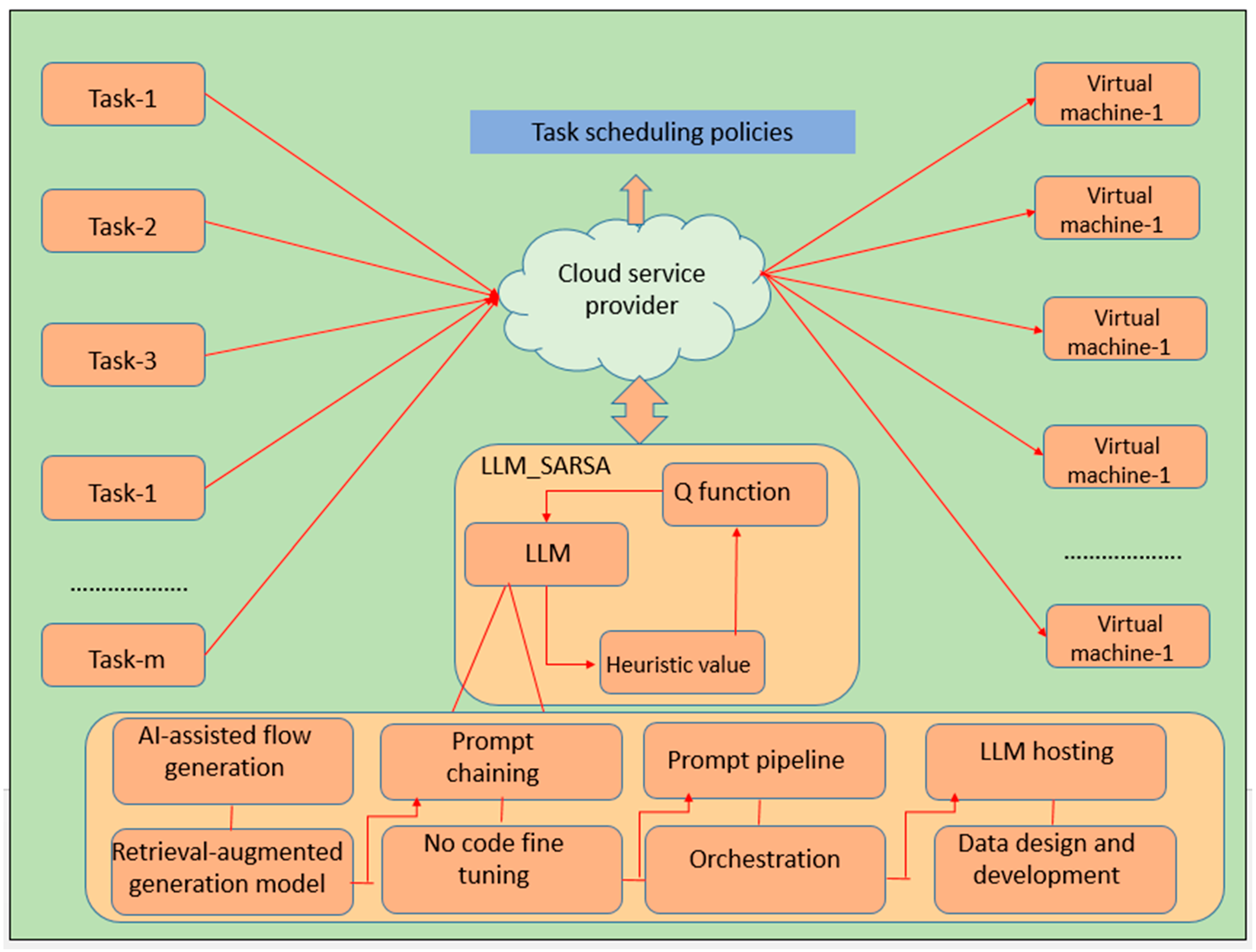
• Employment of the LLM to represent the real-world cloud computing scenario to arrive at better planning and control strategies.
• Illustration of the LLM heuristic value, avoiding the bias in task scheduling policies through significant reshaping of the Q function.
• Proposing a novel LLM-guided SARSA framework along with the supporting algorithm to perform task scheduling.
• Mathematical modeling of an LLM-guided SARSA task scheduler considering the finite cloud scenario and infinite cloud scenario.
• The experimental evaluation of the proposed LLM-guided SARSA task scheduler using the CloudSim express simulator.

The remaining parts of this paper are organized as follows: Section 2 discusses the related work, Section 3 describes the proposed work along with the algorithm, Section 4 performs the mathematical modeling, Section 5 provides a discussion on the results obtained, and finally, Section 6 arrives at the conclusion.

2. Related Work

Wenlong et al. [17] present a dynamic task scheduling framework for a heterogeneous form of a cloud environment using a model-free reinforcement learning algorithm. The cloud system often exhibits a dynamic environment due to its heterogeneity and inherently fluid nature. The task scheduling is performed by using the value iteration method to solve the Bellman equation. The optimal value for each state is determined by taking the best possible actions. Iteratively, the Q value is updated using the Bellman equation until convergence towards an optimal Q value. The accuracy of the value estimation is improved through reward prediction error. Every action value is associated with the predicted reward, and it is updated by propagating the reward prediction error. The explicit knowledge of the system is not taken into consideration to draw optimal policies by incorporating model-free learning methodology. The primary focus is to enhance the reward and cost considerations of the model. The heterogeneity is modeled using the Continuous form of the Time-based Markov Decision Process (CTMDP). It is the collection of a set of variables that are indexed by a continuous quantity of time. The decisions made adhere to the Markov property that the decision of the future variable is dependent on the past variable at any point in time. The explicit trial-and-error mechanism is employed by drawing the policies based on the process data instead of depending on any specific model. The computational efficiency is high as it is not dependent on the potentially flawed or incomplete form of the computing world. The simulation results demonstrate that the proposed model operates very well compared to static scheduling methods. However, the model-free approach suffers from data hunger and is costly as it needs more memory to store the data that are gathered through trial-and-error interaction.

Ramandeep et al. discuss the optimization strategies to improve the performance of task scheduling algorithms [18]. Three optimization techniques are discussed as follows: Tabu search, Bayesian classification, and whale optimization. Tabu search is a heuristic strategy that determines the best resource for the task by utilizing the memory to guide the search process. This prevents the revisiting of the previously explored state and avoids cycling among search states based on tab tenure. Bayesian optimization optimizes the decision making for global optimization, which does not depend on any functional forms. Whale optimization performs optimization using three operators: searching for prey, encircling of the prey, and foraging of the bubble net formation by humpback whales. The proposed algorithm inputs and parses the tasks and allocates ranks by considering the heterogeneous earliest finish time of the tasks. The ranked tasks are distributed among the virtual machines. Tabu search is applied to identify the virtual machine that is less loaded. Bayesian optimization is performed to formulate an effective combination of virtual machines. The population of whales is initialized and the fitness function is updated. If the tasks are optimized, they are migrated; otherwise, the whale optimization is repeated until optimization. From the experimental results, it is found that all three optimization techniques outperform conventional genetic algorithm and particle swarm optimization. However, ranking of tasks by considering the earliest finish time yields better performance but suffers from poor load balancing due to greediness. It is not possible to sacrifice short-term goals to achieve long-term goals. The optimization strategies employed consume a large number of iterations, converge slowly, result in low precision, and also become stuck in local optima.

Wang et al. present a reinforcement learning strategy to perform task scheduling in cloud computing environments [19]. Potential forms of resources include computing power, bandwidth, and storage capacity and the Q learning-based framework is designed to perform optimal task scheduling through efficient utilization of these resources. The intelligent decisions are made by the Q learning agent through past experiences and interactions. The proposed framework first distributes the tasks among the servers dynamically based on the category of the server. Then, the enhanced form of the Q learning algorithm is executed on each server to distribute among the virtual machines. The learning ability of the agent is fine-tuned through reward and punishment mechanisms. During the task assignment stage in the server, priorities are assigned to the task to identify suitable servers. A dynamic sorting process is employed to sort the tasks according to their deadline. The tasks with urgent priority are processed first to provide an improved quality of service. The Upper Confidence Bound algorithm is used to properly balance between the exploration and exploitation phases. It keeps track of the number of iterations a particular action has taken and the performance achieved using the epsilon-greedy policy. Higher efficiency under uncertainty is guaranteed through proper balance between exploration and exploitation using the learned policy. The action with a higher mean value represents the exploration stage and it is selected multiple times. Similarly, the action with a lesser mean value has a wider confidence value, which represents the exploitation stage, and is also selected multiple times. The effectiveness and superiority of the framework are evaluated using various experiments. The performance is found to be good with respect to a reduced makespan time and processing time. However, the chances of arriving at suboptimal solutions are high as it assumes that the rewards are distributed normally, which is not true for this type of scenario. The computational complexity is also high and a high sensitivity is exhibited towards the value chosen for the exploration constant.

Lipsa et al. present a heuristic value and priority-based approach for task scheduling in the cloud [20]. The priority is assigned for each of the incoming tasks by formulating the M/M/n form of the Q learning model. A waiting time matrix assigns the priority for the task upon arrival. The waiting queue incorporates the Fibonacci heap strategy to identify the task exhibiting higher priority. A Fibonacci heap is formed through the collection of several trees that satisfy the minimum heap property. The key value of the child node is always greater than the key value of the parent node. Non-preemptive tasks are considered to conserve both memory and time. Also, early preemption of tasks that are less efficient with respect to the CPU time and memory can also be avoided. A parallel algorithm is designed, which performs priority assignment and heap construction by considering both preemptive and non-preemptive tasks. Different types of errors occur while executing parallel algorithms, which include task error, heap error, runtime error, and so on. These errors are handled by using try catch blocks, which reconstruct the heap upon the occurrence of error. The priority of each task in the waiting queue is increased after every preemption by a small amount. This makes sure that none of the tasks wait for an infinite period of time and assures the convergence of the algorithm. The priority assignment and heap construction are performed concurrently along with the task scheduling. Initially, the number of tasks is empty; heap construction is performed first and then the task scheduling. The experimental results ensure that the proposed algorithm is good in different scenarios involving many tasks with higher and lower priorities. But the Fibonacci heap consumes more memory as it includes multiple tree formations and also stores additional data for each metadata. The random nature of the heap tree causes poor cache performance that has a significant impact on the overall speed of execution of the algorithm.

Abdel et al. discuss task scheduling strategies that work on the basis of a hybrid form of a differential evolution mechanism [21]. Metaheuristic algorithms are increasingly applied to handle task scheduling problems as they are categorized on nondeterministic polynomial time hard problems for which finding an optimal solution within reasonable time is not possible. Differential evolution is a population-based optimization method that involves operators like mutation, crossover, and selection. Two improvements are carried out for differential evolution, which include improving the scaling factor and exploitation operator. The proposed algorithm works in four stages: initialization, evaluation, adaptive mutation factor, and additional exploitation operator. All initialized solutions are evaluated and a solution with a lesser fitness value is chosen for further optimization towards a better solution. The scaling factor is adaptive in nature, which is responsible for enhancing the exploration and exploitation phases of the algorithm. The solutions are updated using a trial vector, which is calculated by considering the current solution and mutant vector. The mutation and crossover operators are helpful to search through the state space and locate effective solutions. Even when the population diversity increases and the generated time steps are high, the scaling factor remains constant. This makes the algorithm find the best solution in the region that is far from the current solution with a near-optimal solution. The experiments are carried out using randomly generated datasets and are found to reduce the makespan time and execution time. However, the scheduler performs very well during initial iterations but during later iterations, it is subjected to improper adaptation of parameters and population stagnation problems.

Nabi et al. present an adaptive form of the particle swarm optimization technique to perform task scheduling in the cloud [22]. The two best positions of the solution are determined using global and local search mechanisms. Proper balance between global and local search is performed by adjusting the inertia weight parameter. The suitable value for the inertia weight parameter is chosen via a linearly descending and adaptive form of the fine-tuning process. The social behavior of the particles is mimicked as inspired by the behavior of flocks of birds and schools of fish. In order to obtain an ideal solution at the beginning of the search procedure itself, it is made sure that the espousal value of the global search space is higher than the espousal value of the local search space. The weight is initialized to be a large value in the beginning to explore the search space exhaustively. The weight value is decreased gradually to decrease the search space that leads to better performance. The best part of the inertia weight strategy is its simplicity and fast convergence rate. The search space is monitored, and the weight values are adjusted by considering the feedback from a few other parameters. The success rate of the particles is considered as feedback to achieve balance between exploration and exploitation. The performance results show a significant reduction in the makespan time is achieved and an enhancement in throughput. However, the inertia weight strategy works well on smaller datasets and suffers from poor performance issues when exposed to larger datasets. Most of the Internet of Things (IoT) devices expect the real-time response time to arrive at a better conclusion. But the proposed scheduler is not tested over delay-sensitive applications with respect to the response time. This limits the practical application of the approach.

A comparison of the existing works with respect to performance is shown in

Table 1. High-level comparison of the existing works in terms of performance.

Technique	Logic	Makespan Time	Degree of Imbalance	Cost	Resource Utilization
Reinforcement learning [17,19]	Trial and error	High	High	Very High	Low
Optimization strategy [18]	Tabu search	High	Very High	Very High	Medium
Metaheuristic strategy [20,21,22]	Popuation-based optimization	Medium	High	Medium	Low

.

To summarize, the drawbacks exhibited by the papers in the literature are as follows.

• The task scheduling optimization strategies developed using traditional metaheuristic algorithms consume too many operations, suffer from slow convergence, and often become stuck in local optima.
• Even hybrid forms of the metaheuristics task schedulers consume a large number of training iterations, suffer from slow convergence, and often become stuck in local optima.
• The reinforcement approaches often exhibit high computational complexity and hypersensitivity towards the exploration constant.
• The model-free approaches are data hungry and exhibit poor efficiency since the input data are gathered through trial-and-error mechanisms.
• The machine learning-based task schedulers do not satisfy the real-time response time requirement of IoT devices.
• Swarm optimization techniques end up with a high response time when evaluated over delay-sensitive applications.

3. System Model

The cloud computing system CCS is composed of m tasks $T=\{t_1,t_2,\dots ,t_m\}$, and n virtual machines $VM=\{{vm}_1,{vm}_2,\dots ,{vm}_n\}$. The performance objectives (POs) are as follows.

PO1: Makespan time: the makespan time of the LLM_SARSA represents the maximum time needed for completing the execution of all the tasks, where $t_i\in \{t_1,t_2,\dots ,t_m\}$ represent the independent tasks that are executed in parallel, $FT\left(t_i\right)$ is the finish time of the independent task $t_i$.

$$MST\left(LL{M}_{SARSA}\right)={Max\_FT}_{t_i\in \left\{t_1,t_2,\dots ,t_m\right\}} \{FT\left(t_i\right) \}$$

(1)

PO2: Degree of imbalance: the degree of imbalance of the LLM_SARSA is the measure of the ratio of the imbalanced load among the virtual machines with the host machine, where ${LD}_{max}\left({vm}_i\right)$ is the maximum load on the virtual machine, ${LD}_{min}\left({vm}_i\right)$ is the minimum load on the virtual machine, and ${LD}_{avg}\left({vm}_i\right)$ is the average load on the virtual machine.

$$DI\left(LLM\_SARSA\right)=Minimize\left(\sum _{i=1}^{i=n}{\displaystyle \frac{{LD}_{max}\left({vm}_i\right)+{LD}_{min}\left({vm}_i\right)}{{LD}_{avg}\left({vm}_i\right)}}\right)$$

(2)

The load on the virtual machine is determined by considering the length of the task set assigned to the virtual machine $TL\{t_i,t_i,t_i\dots ,t_i\}\to {vm}_i$, capacity of the virtual machine $CP\left({vm}_i\right)$

$$LD\left({vm}_i\right)=Balance\left(\sum _{i=1}^m\sum _{j=1}^n{\displaystyle \frac{TL\left\{t_i,t_i,t_i\dots ,t_i\right\}\to {vm}_i}{CP\left({vm}_i\right)}}\right)$$

(3)

PO3: Cost: the cost of the LLM_SARSA is determined by computing the product of the number of tasks mapped on to the virtual machine $N(t_i\to {vm}_j)$ and the cost incurred per unit of time for execution of the assigned task $cost(t_i\to {vm}_j)$.

$$Cost\left(LLM\_SARSA\right)=Minimize\left(\sum _{i=1}^{i=m}\sum _{j=1}^{j=n}N(t_i\to {vm}_j)\ast cost(t_i\to {vm}_j)\right)$$

(4)

PO4: Resource utilization: resource utilization of the LLM_SARSA is measured by considering the resources of the virtual machine that are underutilized ${vm}_i^{under}$ and the resources that are overutilized ${vm}_i^{over}$ over the total number of virtual machines ${TN}_{vm}$.

$$RU\left(LLM\_SARSA\right)=\mathrm{m}\mathrm{a}\mathrm{x}\mathrm{i}\mathrm{m}\mathrm{i}\mathrm{z}\mathrm{e}\left(\sum _{i=1}^{i=n}\left({\displaystyle \frac{{vm}_i^{under}}{{TN}_{vm}}}\ast {\displaystyle \frac{{vm}_i^{over}}{{TN}_{vm}}}\right) \right)$$

(5)

4. Proposed Work

The high-level architecture of the proposed LLM-guided SARSA task scheduler framework is shown in Figure 1. We feel that this framework is suitable for use by cloud service providers (Google cloud, Amazon web service, Microsoft Azure, etc.) to formulate task scheduling policies. The LLM-guided SARSA module is placed within the cloud service provider to process the incoming tasks based on the heuristic values of the Q function. It inputs the incoming task requests with varying resource requirements. The Q value function of a Q learning agent is obtained by computing the cumulative sum of the future rewards of the current action. But the typical Q learning agent’s performance is inefficient over the large state space as it becomes impossible to perform with the growing size of the Q table. This drawback is overcome through the LLM-generated heuristic value, which performs proper Q shaping by estimating the accurate Q value at each step of learning. The LLM model operates in the following steps: AI-assisted flow generation, prompt chaining, orchestration, and LLM hosting. The LLM model is prompted with both good and bad samples of state pairs of the task and virtual machine pairs to arrive at the precise heuristic value. Through LLM guidance, the SARSA module is capable of formulating optimal task scheduling policies and does not become trapped in sub-optimal solutions. The heuristic value is used to reshape the Q function, which nullifies the effect of hallucination and avoids the over- and underestimations of the Q value function. This in turn increases the convergence rate of the Q learning agent.

The detailed working of each of the functional modules of the LLM_SARSA task scheduler is provided in Algorithm 1. The algorithm operates in two stages: training and testing. The task set is input and allotted to best fit virtual machines using the task scheduling policies of the LLM-enriched SARSA logic. By embedding the heuristic value generated by the LLM, the Q function is modulated to generate the desired policies. The Q function is reshaped by considering the loss function and heuristic value, which converge to the optimal Q state. The improved sampling efficiency and better tuning of hyperparameters increases the adaptability of the scheduler and also prevents improper exploration of the state space.

Algorithm 1: Working of LLM_SARSA task scheduler

1: Start 2: Input: Input the set of task           $\mathit{T}=\{{\mathit{t}}_1,{\mathit{t}}_2,{\mathit{t}}_3,{\mathit{t}}_4,\dots ,{\mathit{t}}_{\mathit{m}}\}$ 3: Output: Output task scheduling policies          $\mathsf{\Pi }\mathit{P}=\{{\mathsf{\Pi }\mathit{P}}_1,{\mathsf{\Pi }\mathit{P}}_2,{\mathsf{\Pi }\mathit{P}}_3,{\mathsf{\Pi }\mathit{P}}_4,{\mathsf{\Pi }\mathit{P}}_5\dots ,{\mathsf{\Pi }\mathit{P}}_{\mathit{p}}\}$ 4: Initialize $\mathit{Q}\left(\mathit{s},\mathit{a}\right),\forall \mathit{s}\in \mathit{S},\mathit{a}\in \mathit{A}\left(\mathit{s}\right),\mathbf{a}\mathbf{r}\mathbf{b}\mathbf{i}\mathbf{t}\mathbf{r}\mathbf{a}\mathbf{r}\mathbf{i}\mathbf{l}\mathbf{y} \mathbf{a}\mathbf{n}\mathbf{d} \mathbf{Q}\left(\mathbf{t}\mathbf{e}\mathbf{r}\mathbf{m}\mathbf{i}\mathbf{n}\mathbf{a}\mathbf{l} \mathbf{s}\mathbf{t}\mathbf{a}\mathbf{t}\mathbf{e}\right)=0$ 5: Initialize LLM heuristic Q buffer $\mathit{D}\left(\mathit{G}\right(\mathit{p})=\{({\mathit{S}}_{\mathit{i}},{\mathit{A}}_{\mathit{i}},{\mathit{Q}}_{\mathit{i}})|\left({\mathit{S}}_{\mathit{i}},{\mathit{A}}_{\mathit{i}},{\mathit{Q}}_{\mathit{i}}\right)\in \mathit{D}\left(\mathit{G}\left(\mathit{p}\right)\right),\mathit{i}=\mathrm{1,2}\dots \mathit{n}\}$ 6: For each episode S, perform 7:   Training phase of LLM_SARSA 8:        For every task in training task set ${\mathit{t}}_{\mathit{i}}\in \mathit{T},$ perform 9:        Initialize state S, Action A 10:      Choose Action A from state S using the policy derived from $\in \mathit{g}\mathit{r}\mathit{e}\mathit{e}\mathit{d}\mathit{y}$ 11:        For each step of episode, perform 12:         Take action A, observe reward R, and go to next step ${\mathit{S}}^{\prime }$ 13:         Choose action ${\mathit{A}}^{\prime }$ from state ${\mathit{S}}^{\prime }$ using the policy derived from $\in \mathit{g}\mathit{r}\mathit{e}\mathit{e}\mathit{d}\mathit{y}$ 11:      $\mathit{Q}\left(\mathit{S},\mathit{A}\right)=\mathit{Q}\left(\mathit{S},\mathit{A}\right)+\mathit{\alpha }(\mathit{R}+\mathit{\gamma }\ast \mathit{Q}\left({\mathit{S}}^{\prime },{\mathit{A}}^{\prime }\right)-\mathit{Q}(\mathit{S},\mathit{A})$ 12:          Update $\mathit{S}\leftarrow {\mathit{S}}^{\prime }$, $\mathit{A}\leftarrow {\mathit{A}}^{\prime }$ 12:          Compute the LLM heuristic value $\mathit{D}(\mathit{G}\left(\mathit{p}\right)=\mathit{D}(\mathit{G}\left(\mathit{p}\right)\cup \mathit{Q}\left(\mathit{S},\mathit{A},\mathit{R},{\mathit{S}}^{\prime }\right)$ 13:          Update the $\mathit{Q}\left(\mathit{S},\mathit{A}\right)$ with LLM $\mathit{D}(\mathit{G}\left(\mathit{p}\right)$ 14:          ${\mathit{Q}}^{\mathit{*}}\left(\mathit{S},\mathit{A}\right)=(\mathit{Q}\left(\mathit{S},\mathit{A}\right)+\mathit{\alpha }(\mathit{R}+\mathit{\gamma }\ast \mathit{Q}\left({\mathit{S}}^{\prime },{\mathit{A}}^{\prime }\right)-\mathit{Q}\left(\mathit{S},\mathit{A}\right))+\mathit{D}(\mathit{G}\left(\mathit{p}\right))$ 15:          Employ L2 loss to approximate the ${\mathit{Q}}^{\mathit{*}}$ value 16:          L2(${\mathit{Q}}^{\mathit{*}}\left(\mathit{S},\mathit{A}\right))=\mathit{E}\mathit{r}\mathit{r}\mathit{o}\mathit{r}\left(\mathit{S},\mathit{A},{\mathit{Q}}^{\mathit{*}}\left(\mathit{S},\mathit{A}\right)\right)\ast \mathit{D}(\mathit{G}\left(\mathit{p}\right)\ast {({\mathit{Q}}^{\mathit{*}\mathit{*}}\left(\mathit{S},\mathit{A}\right)-{\mathit{Q}}^{\mathit{*}}\left(\mathit{S},\mathit{A}\right))}^2$ 17:        ${\mathit{Q}}^{\mathit{*}\mathit{*}}\left(\mathit{S},\mathit{A}\right)=\mathbf{L}2({\mathit{Q}}^{\mathit{*}}\left(\mathit{S},\mathit{A}\right))+({\mathit{Q}}^{\mathit{*}}\left(\mathit{S},\mathit{A}\right)+\mathit{\alpha }(\mathit{R}+\mathit{\gamma }\ast {\mathit{Q}}^{\mathit{*}}\left({\mathit{S}}^{\prime },{\mathit{A}}^{\prime }\right)-{\mathit{Q}}^{\mathit{*}}\left(\mathit{S},\mathit{A}\right))+\mathit{D}(\mathit{G}\left(\mathit{p}\right))$ 18:           End For of episode until S is terminal 19:    End For 20:    Testing phase of LLM_SARSA 21:       For every task in testing task set ${\mathit{t}}_{\mathit{i}}\in \mathit{T},$ perform 22:          Initialize state S, Action A 23:          Choose Action A from state S using the policy derived from $\in \mathit{g}\mathit{r}\mathit{e}\mathit{e}\mathit{d}\mathit{y}$ 24:           For each step of episode, perform 25:              Execute the action ${\mathit{A}}^{\prime }$ from state ${\mathit{S}}^{\prime }$ with updated heuristic value and L2 loss value 26:              ${\mathit{Q}}^{\mathit{*}\mathit{*}}\left(\mathit{S},\mathit{A}\right)=\mathbf{L}2({\mathit{Q}}^{\mathit{*}}\left(\mathit{S},\mathit{A}\right))+({\mathit{Q}}^{\mathit{*}}\left(\mathit{S},\mathit{A}\right)+\mathit{\alpha }(\mathit{R}+\ast \mathit{*}{\mathit{Q}}^{\mathit{*}}\left({\mathit{S}}^{\prime },{\mathit{A}}^{\prime }\right)-{\mathit{Q}}^{\mathit{*}}\left(\mathit{S},\mathit{A}\right))+\mathit{D}(\mathit{G}\left(\mathit{p}\right))$ 27:           End For of episode until S is terminal 28:          End For 29: End For 30: Output $\mathsf{\Pi }\mathit{P}=\{{\mathsf{\Pi }\mathit{P}}_1,{\mathsf{\Pi }\mathit{P}}_2,{\mathsf{\Pi }\mathit{P}}_3,{\mathsf{\Pi }\mathit{P}}_4,{\mathsf{\Pi }\mathit{P}}_5\dots ,{\mathsf{\Pi }\mathit{P}}_{\mathit{p}}\}$ 34: Stop

5. Mathematical Modeling

The mathematical modeling of the proposed LLM_SARSA is conducted to measure the makespan time, degree of imbalance, cost, and resource utilization. Two different types of cloud scenarios are considered for modeling purposes: finite and infinite. In a finite cloud scenario, a finite set of tasks and virtual machines are made available, whereas in an infinite cloud scenario, an infinite set of tasks and virtual machines are made available.

5.1. Finite Cloud Scenario

The finite cloud scenario consists of m number of tasks $T=\{t_1,t_2,\dots ,t_m\}$, where <= I <= m number of virtual machines $VM=\{{vm}_1,{vm}_2,\dots ,{vm}_n\}$, where 1 <= j <= n. The P task scheduling policies are formulated, $\mathsf{\Pi }P=<{\mathsf{\Pi }P}_1,{\mathsf{\Pi }P}_2,{\mathsf{\Pi }P}_3,{\mathsf{\Pi }P}_4,{\mathsf{\Pi }P}_5\dots ,{\mathsf{\Pi }P}_p>$. The output is computed for three time intervals, i.e., $<T>,<T+\alpha >,<T+2\alpha >$ and it ranges between low, medium, or high, i.e., $\mathrm{P}\_\mathrm{O}\mathrm{P}=<low, medium, high>$.

PO1: Makespan time: The expected value of the makespan time $EV\left(MST\right(LLM\_SARA\left)\right)$ is directly proportional to the expected value of the finish time of the independent tasks $EV\left(FT\left(t_i\right)\right))$, where the task ranges from $iϵ\{1, 2, 3,\dots ,k\}$. The derivation of the makespan time under the finite cloud scenario is given in

Table 2. Makespan time under finite cloud scenario.

$EV\left({\displaystyle \frac{MST\left(LLM\_SARSA\right)}{LLM\_SARSA\left(\mathsf{\Pi }P\right)}}, T\right)={\int }_x^y{\displaystyle \frac{\sum _{aϵ\pi p}{Max\_FT}_{\left(t_i\right)\in \{\mathrm{1,2},3..,k\}} \left\{FT\left(t_i\right)\right\}\left(a\right)}{|LLM\_SARSA(\mathsf{\Pi }P\left)\right|}}$	$\left(6\right)$
$EV\left({\displaystyle \frac{MST\left(LLM\_SARSA\right)}{LLM\_SARSA\left(\mathsf{\Pi }P\right)}}, T\right)={\displaystyle \sum _{d\in D}}d{\int }_x^y{\displaystyle \frac{\sum _{aϵp\pi }{Ma{x}_{FT}}_{\left(t_i\right)\in \left\{\mathrm{1,2},3..,k\right\}} \left\{FT\left(t_i\right)\right\}\left(a\right)}{\left|LL{M}_{SARSA\left(\mathsf{\Pi }P\right)}\right|}}$	$\left(7\right)$
$EV\left({\displaystyle \frac{MST\left(LLM\_SARSA\right)}{LLM\_SARSA\left(\mathsf{\Pi }P\right)}}, T\right)={\displaystyle \frac{EV\left(1\ast p\pi \ast \sum _{i=1}^{i=n}{Ma{x}_{FT}}_{t_i\in \left\{\mathrm{1,2},3..,k\right\}} \left\{FT\left(t_i\right)\right\}\right)}{P\left(LL{M}_{SARSA\left(\mathsf{\Pi }P\right)}\right)}}$	$\left(8\right)$
$EV\left({\displaystyle \frac{MST\left(LLM\_SARSA\right)}{LLM\_SARSA\left(\mathsf{\Pi }P\right)}}, T\right)={\displaystyle \sum _{d\in D}}d{\int }_q^Q{Max\_FT}_{t_i\in \{\mathrm{1,2},3..,k\}} \left\{FT\left(t_i\right)\right\}$	$\left(9\right)$
$EV\left({\displaystyle \frac{MST\left(LLM\_SARSA\right)}{LLM\_SARSA\left(\mathsf{\Pi }P\right)}}, T\right)={\int }_q^{Q}Q\ast dP{\displaystyle \frac{{Max\_FT}_{t_i\in \{\mathrm{1,2},3..,k\}} \left\{FT\left(t_i\right)\right\}}{LLM\_SARSA\left(\mathsf{\Pi }P\right)}}$	$\left(10\right)$
$EV\left({\displaystyle \frac{MST\left(LLM\_SARSA\right)}{LLM\_SARSA\left(\mathsf{\Pi }P\right)}}, T\right)\cong Low$	$\left(11\right)$
$EV\left({\displaystyle \frac{MST\left(LL{M}_{SARSA}\right)}{LL{M}_{SARSA\left(\mathsf{\Pi }P\right)}}}, T+\alpha \right)\cong Medium$	$\left(12\right)$
$EV\left({\displaystyle \frac{MST\left(LL{M}_{SARSA}\right)}{LL{M}_{SARSA\left(\mathsf{\Pi }P\right)}}}, T+2\alpha \right)\cong Low$	$\left(13\right)$

.

PO2: Degree of imbalance: The expected value of the makespan time $EV\left(DI\right(LLM\_SARSA\left)\right)$ is directly proportional to the expected value of the maximum load on the virtual machine $EV\left({LD}_{max}\left({vm}_i\right)\right)$, minimum load on the virtual machine $EV\left({LD}_{min}\left({vm}_i\right)\right)$, and average load on the virtual machine ${EV(LD}_{avg}\left(\left({vm}_i\right)\right)$. The derivation of the degree of imbalance under the finite cloud scenario is given in

Table 3. Degree of imbalance under finite cloud scenario.

$EV\left({\displaystyle \frac{DI\left(LLM\_SARSA\right)}{LLM\_SARSA\left(\mathsf{\Pi }P\right)}}, T\right)={\displaystyle \sum _{d\in D}}d{\int }_x^y{\displaystyle \frac{{\sum }_{aϵp\pi }DI\left(LL{M}_{SARSA}\right)\left(a\right)}{\left|LL{M}_{SARSA\left(\mathsf{\Pi }P\right)}\right|}}$	$\left(14\right)$
$EV\left({\displaystyle \frac{DI\left(LLM\_SARSA\right)}{LLM\_SARSA\left(\mathsf{\Pi }P\right)}}, T\right)={\displaystyle \frac{E\left(1\ast \pi \ast \sum _{i=1}^{i=n}\frac{{LD}_{max}\left({vm}_i\right)+{LD}_{min}\left({vm}_i\right)}{{LD}_{avg}(\left({vm}_i\right)}\right)}{P\left(LL{M}_{SARSA\left(\mathsf{\Pi }P\right)}\right)}}$	$\left(15\right)$
$EV\left({\displaystyle \frac{DI\left(LLM\_SARSA\right)}{LLM\_SARSA\left(\mathsf{\Pi }P\right)}}, T\right)={\displaystyle \sum _{d\in D}}d{\int }_q^Q{\displaystyle \sum _{i=1}^{i=n}}{\displaystyle \frac{{LD}_{max}\left({vm}_i\right)+{LD}_{min}\left({vm}_i\right)}{{LD}_{avg}(\left({vm}_i\right)}}$	$\left(16\right)$
$EV\left({\displaystyle \frac{DI\left(LLM\_SARSA\right)}{LLM\_SARSA\left(\mathsf{\Pi }P\right)}}, T\right)={\int }_q^{Q}Q\ast dP{\displaystyle \frac{\sum _{i=1}^{i=n}\frac{{LD}_{max}\left({vm}_i\right)+{LD}_{min}\left({vm}_i\right)}{{LD}_{avg}(\left({vm}_i\right)}}{LL{M}_{SARSA\left(\mathsf{\Pi }P\right)}}}$	$\left(17\right)$
$EV\left({\displaystyle \frac{DI\left(LL{M}_{SARSA}\right)}{LL{M}_{SARSA\left(\mathsf{\Pi }P\right)}}}, T\right)\cong Low$	$\left(18\right)$
$EV\left({\displaystyle \frac{DI\left(LLM\_SARSA\right)}{LLM\_SARSA\left(\mathsf{\Pi }P\right)}}, T+\alpha \right)\cong Medium$	$\left(19\right)$
and $EV\left({\displaystyle \frac{DI\left(LLM\_SARSA\right)}{LLM\_SARSA\left(\mathsf{\Pi }P\right)}}, T+2\alpha \right)\cong Low$	$\left(20\right)$

.

PO3: Cost: The expected value of the cost $EV\left(Cost\right(LLM\_SARSA\left)\right)$ is influenced by the expected value of the number of tasks on the virtual machine $EV\left(N\left(t_i\to {vm}_j\right)\right)$ and expected value of the cost incurred per unit of time for execution of the assigned task $EV\left(cost\left(t_i\to {vm}_j\right)\right)$. The derivation of the cost under the finite cloud scenario is given in

Table 4. Cost under finite cloud scenario.

$EV\left({\displaystyle \frac{Cost(LLM\_SARSA)}{LLM\_SARSA\left(\mathsf{\Pi }P\right)}}, T\right)={\int }_x^y{\displaystyle \frac{\sum _{aϵp\pi }Cost(LLM\_SARSA)\left(a\right)}{|LLM\_SARSA(\mathsf{\Pi }P\left)\right|}}$	$\left(21\right)$
$EV\left({\displaystyle \frac{Cost(LLM\_SARSA)}{LLM\_SARSA\left(\mathsf{\Pi }P\right)}}, T\right)={\displaystyle \sum _{d\in D}}d{\int }_x^y{\displaystyle \frac{\sum _{aϵ\pi }Cost(LLM\_SARSA)\left(a\right)}{|LLM\_SARSA(\mathsf{\Pi }P\left)\right|}}$	$\left(22\right)$
$EV\left({\displaystyle \frac{Cost(LLM\_SARSA)}{LLM\_SARSA\left(\mathsf{\Pi }P\right)}}, T\right)={\displaystyle \frac{E\left(1\ast \pi \ast \sum _{i=1}^{i=n}Cost(LLM\_SARSA)\right)}{P(LLM\_SARSA(\mathsf{\Pi }P\left)\right)}}$	$\left(23\right)$
$EV\left({\displaystyle \frac{Cost(LLM\_SARSA)}{LLM\_SARSA\left(\mathsf{\Pi }P\right)}}, T\right)={\displaystyle \sum _{d\in D}}d{\int }_q^Q{\displaystyle \sum _{i=1}^{i=m}}{\displaystyle \sum _{j=1}^{j=n}}N(t_i\to {vm}_j)\ast cost\left(t_i\to {vm}_j\right)$	$\left(24\right)$
$EV\left({\displaystyle \frac{Cost(LLM\_SARSA)}{LLM\_SARSA\left(\mathsf{\Pi }P\right)}}, T\right)={\int }_q^{Q}Q\ast dP{\displaystyle \frac{\left[ \left(\sum _{i=1}^{i=m}\sum _{j=1}^{j=n}N(t_i\to {vm}_j)\ast cost(t_i\to {vm}_j)\right)\right]}{LL{M}_{SARSA\left(\mathsf{\Pi }P\right)}}}$	$\left(25\right)$
$EV\left({\displaystyle \frac{Cost\left(LLM\_SARSA\right)}{LLM\_SARSA\left(\mathsf{\Pi }P\right)}}, T\right)\cong Low$	$\left(26\right)$
$EV\left({\displaystyle \frac{Cost\left(LLM\_SARSA\right)}{LLM\_SARSA\left(\mathsf{\Pi }P\right)}}, T+\alpha \right)\cong Low$	$\left(27\right)$
and $EV\left({\displaystyle \frac{COst\left(LLM\_SARSA\right)}{LLM\_SARSA\left(\mathsf{\Pi }P\right)}}, T+2\alpha \right)\cong Medium$	$\left(28\right)$

.

PO4: Resource utilization: The expected value of the resource utilization $EV\left(RU\right(LLM\_SARA\left)\right)$ is directly proportional to the expected value of the underutilized virtual machine resources ${EV(vm}_i^{under})$, overutilized virtual machine resources ${EV(vm}_i^{over})$, and total number of virtual machines ${EV(TN}_{vm})$. The derivation of the resource utilization under the finite cloud scenario is shown in

Table 5. Resource utilization under finite cloud scenario.

$EV\left({\displaystyle \frac{RU(LLM\_SARSA)}{LLM\_SARSA\left(\mathsf{\Pi }P\right)}}, T\right)={\int }_x^y{\displaystyle \frac{\sum _{aϵ\pi }RU(LLM\_SARSA)\left(a\right) }{|LLM\_SARSA(\mathsf{\Pi }P\left)\right|}}$	$\left(29\right)$
$EV\left({\displaystyle \frac{RU(LLM\_SARSA)}{LLM\_SARSA\left(\mathsf{\Pi }P\right)}}, T\right)={\displaystyle \sum _{d\in D}}d{\int }_x^y{\displaystyle \frac{\sum _{aϵ\pi }RU(LLM\_SARSA)\left(a\right)}{|LLM\_SARSA(\mathsf{\Pi }P\left)\right|}}$	$\left(30\right)$
$EV\left({\displaystyle \frac{RU(LLM\_SARSA)}{LLM\_SARSA\left(\mathsf{\Pi }P\right)}}, T\right)={\displaystyle \frac{EV\left(1\ast \pi \ast \sum _{i=1}^{i=n}RU(LLM\_SARSA)\right)}{P(LLM\_SARSA(\mathsf{\Pi }P\left)\right)}}$	$\left(31\right)$
$EV\left({\displaystyle \frac{RU(LLM\_SARSA)}{LLM\_SARSA\left(\mathsf{\Pi }P\right)}}, T\right)={\displaystyle \sum _{d\in D}}d{\int }_q^Q{\displaystyle \sum _{i=1}^{i=m}}\left({\displaystyle \frac{{vm}_i^{under}}{{TN}_{vm}}}\ast {\displaystyle \frac{{vm}_i^{over}}{{TN}_{vm}}}\right)$	$\left(32\right)$
$EV\left({\displaystyle \frac{RU(LLM\_SARSA)}{LLM\_SARSA\left(\mathsf{\Pi }P\right)}}, T\right)={\int }_q^{Q}Q\ast dP{\displaystyle \frac{\sum _{i=1}^{i=m}\left(\frac{{vm}_i^{under}}{{TN}_{vm}}\ast \frac{{vm}_i^{over}}{{TN}_{vm}}\right) }{LL{M}_{SARSA\left(\mathsf{\Pi }P\right)}}}$	$\left(33\right)$
$EV\left({\displaystyle \frac{RU\left(LLM\_SARSA\right)}{LLM\_SARSA\left(\mathsf{\Pi }P\right)}}, T\right)\cong Low$	$\left(34\right)$
$EV\left({\displaystyle \frac{RU\left(LLM\_SARSA\right)}{LLM\_SARSA\left(\mathsf{\Pi }P\right)}}, T+\alpha \right)\cong Low$	(35)
and $EV\left({\displaystyle \frac{RU\left(LLM\_SARSA\right)}{LLM\_SARSA\left(\mathsf{\Pi }P\right)}}, T+2\alpha \right)\cong Medium$	$\left(36\right)$

.

5.2. Infinite Cloud Scenario

The infinite cloud scenario consists of $\infty$ number of tasks $T=\{t_1,t_2,\dots ,t_{\infty }\}$, where 1 <= i <=$\infty$ number of virtual machines $VM=\{{vm}_1,{vm}_2,\dots ,{vm}_{\infty }\}$, where 1 <= j <=$\infty$. The P task scheduling policies are formulated $\mathrm{T}\mathrm{S}P=<{TSP}_1,{TSP}_2,{TSP}_3,{TSP}_4,{TSP}_5\dots ,{TSP}_p>$. The output is computed for three time intervals, i.e., $<T>,<T+\alpha >,<T+2\alpha >$ and it ranges between low, medium, or high, i.e., $\mathrm{P}\_\mathrm{O}\mathrm{S}=<low, medium, high>$.

PO1: Makespan time: In comparison with the finite cloud scenario, the expected value of the makespan time consistently remains low in the infinite cloud scenario. The derivation of the makespan time under the infinite cloud scenario is shown in

Table 6. Makespan time under infinite cloud scenario.

${EV}^{\prime }\left({\displaystyle \frac{MST(LLM\_SARSA)}{LLM\_SARSA\left(\mathsf{\Pi }P\right)}}, T\right)={\int }_{-\infty }^0{\displaystyle \frac{\sum _{aϵ\pi }MST(LLM\_SARSA)\left(a\right)}{|LLM\_SARSA(\mathsf{\Pi }P\left)\right|}}+{\int }_0^{+\infty }{\displaystyle \frac{\sum _{aϵ\pi }MST(LLM\_SARSA)\left(a\right)}{|LLM\_SARSA(\mathsf{\Pi }P\left)\right|}}$	$\left(37\right)$
${EV}^{\prime }\left({\displaystyle \frac{MST\left(LL{M}_{SARSA}\right)}{LL{M}_{SARSA\left(\mathsf{\Pi }P\right)}}}, T\right)={\displaystyle \sum _{d\in D}}d{\int }_{-\infty }^0{\displaystyle \frac{\sum _{aϵ\pi }MST\left(LL{M}_{SARSA}\right)\left(a\right)}{\left|LL{M}_{SARSA\left(\mathsf{\Pi }P\right)}\right|}}+$ ${\int }_0^{+\infty }{\displaystyle \frac{\sum _{aϵ\pi }MST(LLM\_SARSA)\left(a\right)}{|LLM\_SARSA(\mathsf{\Pi }P\left)\right|}}$	$\left(38\right)$
${EV}^{\prime }\left({\displaystyle \frac{MST(LLM\_SARSA)}{LLM\_SARSA\left(\mathsf{\Pi }P\right)}}, T\right)={\int }_{-\infty }^{+\infty }{\displaystyle \frac{{EV}^{\prime }\left(1\ast p\pi \ast \sum _{i=1}^{i=n}{Max\_FT}_{\left(t_i\right)\in \{\mathrm{1,2},3..,k\}} \left\{FT\left(t_i\right)\right\}\right)}{P(LLM\_SARSA(\mathsf{\Pi }P\left)\right)}}$	$\left(39\right)$
${EV}^{\prime }\left({\displaystyle \frac{MST(LLM\_SARSA)}{LLM\_SARSA\left(\mathsf{\Pi }P\right)}}, T\right)\cong Low\cong EV\left({\displaystyle \frac{MS{T}_{FT\left(LL{M}_{SARSA}\right)}}{LL{M}_{SARSA\left(\mathsf{\Pi }P\right)}}}, T\right)\cong Low$	$\left(40\right)$
${EV}^{\prime }\left({\displaystyle \frac{MST(LLM\_SARSA)}{LLM\_SARSA\left(\mathsf{\Pi }P\right)}}, T+\alpha \right)\cong Medium\le EV\left({\displaystyle \frac{MS{T}_{FT\left(LL{M}_{SARSA}\right)}}{LL{M}_{SARSA\left(\mathsf{\Pi }P\right)}}}, T+\alpha \right) \cong Low$	$\left(41\right)$
${EV}^{\prime }\left({\displaystyle \frac{MST(LLM\_SARSA)}{LLM\_SARSA\left(\mathsf{\Pi }P\right)}}, T+2\alpha \right)\cong Low\cong EV\left({\displaystyle \frac{MS{T}_{FT\left(LL{M}_{SARSA}\right)}}{LL{M}_{SARSA\left(\mathsf{\Pi }P\right)}}}, T+2\alpha \right)\cong Low$	$\left(42\right)$

.

PO2: Degree of imbalance: In comparison with the finite cloud scenario, the expected value of the degree of imbalance reduces significantly in the infinite cloud scenario. The derivation of the degree of imbalance under the infinite cloud scenario is shown in

Table 7. Degree of imbalance under infinite cloud scenario.

${EV}^{\prime }\left({\displaystyle \frac{DI(LLM\_SARSA)}{LLM\_SARSA\left(\mathsf{\Pi }P\right)}}, T\right)={\int }_{-\infty }^0{\displaystyle \frac{\sum _{aϵ\pi }DI(LLM\_SARSA)\left(a\right)}{|LLM\_SARSA(\mathsf{\Pi }P\left)\right|}}+{\int }_0^{+\infty }{\displaystyle \frac{\sum _{aϵ\pi }DI\left(LL{M}_{SARSA}\right)\left(a\right)}{\left|LL{M}_{SARSA\left(\mathsf{\Pi }P\right)}\right|}}$	$\left(43\right)$
${EV}^{\prime }\left({\displaystyle \frac{DI(LLM\_SARSA)}{LLM\_SARSA\left(\mathsf{\Pi }P\right)}}, T\right)={\displaystyle \sum _{d\in D}}d{\int }_{-\infty }^0{\displaystyle \frac{\sum _{aϵ\pi }DI(LLM\_SARSA)\left(a\right)}{|LLM\_SARSA(\mathsf{\Pi }P\left)\right|}}+{\int }_0^{+\infty }{\displaystyle \frac{\sum _{aϵ\pi }DI(LLM\_SARSA)\left(a\right)}{|LLM\_SARSA(\mathsf{\Pi }P\left)\right|}}$	$\left(44\right)$
${EV}^{\prime }\left({\displaystyle \frac{DI(LLM\_SARSA)}{LLM\_SARSA\left(\mathsf{\Pi }P\right)}}, T\right)={\int }_{-\infty }^{+\infty }{EV}^{\prime }\left({\displaystyle \sum _{i=1}^{i=n}}{\displaystyle \frac{{LD}_{max}\left({vm}_i\right)+{LD}_{min}\left({vm}_i\right)}{{LD}_{avg}(\left({vm}_i\right)}}\right)$	$\left(45\right)$
${EV}^{\prime }\left({\displaystyle \frac{DI(LLM\_SARSA)}{LLM\_SARSA\left(\mathsf{\Pi }P\right)}}, T\right)\cong Low\cong EV\left({\displaystyle \frac{DI\left(LL{M}_{SARSA}\right)}{LL{M}_{SARSA\left(\mathsf{\Pi }P\right)}}}, T\right)\cong Low$	$\left(46\right)$
${EV}^{\prime }\left({\displaystyle \frac{DI(LLM\_SARSA)}{LLM\_SARSA\left(\mathsf{\Pi }P\right)}}, T+\alpha \right)\cong Medium\to EV\left({\displaystyle \frac{DI\left(LL{M}_{SARSA}\right)}{LL{M}_{SARSA\left(\mathsf{\Pi }P\right)}}}, T+\alpha \right)\cong Medium$	$\left(47\right)$
${EV}^{\prime }\left({\displaystyle \frac{DI(LLM\_SARSA)}{LLM\_SARSA\left(\mathsf{\Pi }P\right)}}, T+2\alpha \right)\cong Low\cong EV\left({\displaystyle \frac{DI\left(LL{M}_{SARSA}\right)}{LL{M}_{SARSA\left(\mathsf{\Pi }P\right)}}}, T+2\alpha \right)\cong Low$	$\left(48\right)$

.

PO3: Cost: In comparison with the finite cloud scenario, the expected value of the cost remains in the moderate range in the infinite cloud scenario. The derivation of the cost under the infinite cloud scenario is shown in

Table 8. Cost under infinite cloud scenario.

${EV}^{\prime }\left({\displaystyle \frac{Cost(LLM\_SARSA)}{LLM\_SARSA\left(\mathsf{\Pi }P\right)}}, T\right)={\int }_{-\infty }^0{\displaystyle \frac{\sum _{aϵ\pi }Cost(LLM\_SARSA)\left(a\right)}{|LLM\_SARSA(\mathsf{\Pi }P\left)\right|}}+{\int }_0^{+\infty }{\displaystyle \frac{\sum _{aϵ\pi }Cost\left(LL{M}_{SARSA}\right)\left(a\right)}{\left|LL{M}_{SARSA\left(\mathsf{\Pi }P\right)}\right|}}$	$\left(49\right)$
${EV}^{\prime }\left({\displaystyle \frac{Cost\left(LL{M}_{SARSA}\right)}{LL{M}_{SARSA\left(\mathsf{\Pi }P\right)}}}, T\right)={\displaystyle \sum _{d\in D}}d{\int }_{-\infty }^0{\displaystyle \frac{\sum _{aϵ\pi }Cost\left(LL{M}_{SARSA}\right)\left(a\right)}{\left|LL{M}_{SARSA\left(\mathsf{\Pi }P\right)}\right|}}+$ ${\int }_0^{+\infty }{\displaystyle \frac{\sum _{aϵ\pi }Cost(LLM\_SARSA)\left(a\right)}{|LLM\_SARSA(\mathsf{\Pi }P\left)\right|}}$	$\left(50\right)$
${EV}^{\prime }\left({\displaystyle \frac{Cost(LLM\_SARSA)}{LLM\_SARSA\left(\mathsf{\Pi }P\right)}}, T\right)={\displaystyle \sum _{d\in D}}d{\int }_{-\infty }^{+\infty }{\displaystyle \sum _{i=1}^{i=m}}{\displaystyle \sum _{j=1}^{j=n}}{EV}^{\prime }\left(ET\right(t_i\to {vm}_j)\ast cost(t_i\to {vm}_j))$	$\left(51\right)$
${EV}^{\prime }\left({\displaystyle \frac{Cost(LLM\_SARSA)}{LLM\_SARSA\left(\mathsf{\Pi }P\right)}}, T\right)\cong Low\cong EV\left({\displaystyle \frac{Cost\left(LL{M}_{SARSA}\right)}{LL{M}_{SARSA\left(\mathsf{\Pi }P\right)}}}, T\right)\cong Low$	$\left(52\right)$
${EV}^{\prime }\left({\displaystyle \frac{Cost(LLM\_SARSA)}{LLM\_SARSA\left(\mathsf{\Pi }P\right)}}, T+\alpha \right)\cong Low\to EV\left({\displaystyle \frac{Cost\left(LL{M}_{SARSA}\right)}{LL{M}_{SARSA\left(\mathsf{\Pi }P\right)}}}, T+\alpha \right)\cong Low$	$\left(53\right)$
${EV}^{\prime }\left({\displaystyle \frac{Cost(LLM\_SARSA)}{LLM\_SARSA\left(\mathsf{\Pi }P\right)}}, T+2\alpha \right)\cong Medium\le EV\left({\displaystyle \frac{Cost\left(LL{M}_{SARSA}\right)}{LL{M}_{SARSA\left(\mathsf{\Pi }P\right)}}}, T+2\alpha \right)\cong Low$	$\left(54\right)$

.

PO4: Resource utilization: In comparison with the finite cloud scenario, the expected value of the resource utilization consistently remains high in the infinite cloud scenario. The derivation n of the resource utilization under the infinite cloud scenario is shown in

Table 9. Resource utilization under infinite cloud scenario.

${EV}^{\prime }\left({\displaystyle \frac{RU\left(LL{M}_{SARSA}\right)}{LL{M}_{SARSA\left(\mathsf{\Pi }P\right)}}}, T\right)={\int }_{-\infty }^0{\displaystyle \frac{\sum _{aϵ\pi }RU\left(LL{M}_{SARSA}\right)\left(a\right)}{\left|LL{M}_{SARSA\left(\mathsf{\Pi }P\right)}\right|}}+$ ${\int }_0^{+\infty }{\displaystyle \frac{\sum _{aϵ\pi }RU(LLM\_SARSA)\left(a\right)}{|LLM\_SARSA(\mathsf{\Pi }P\left)\right|}}$	$\left(55\right)$
${EV}^{\prime }\left({\displaystyle \frac{RU\left(LL{M}_{SARSA}\right)}{LL{M}_{SARSA\left(\mathsf{\Pi }P\right)}}}, T\right)$ $={\displaystyle \sum _{d\in D}}d{\int }_{-\infty }^0{\displaystyle \frac{\sum _{aϵ\pi }RU(LLM\_SARSA)\left(a\right)}{|LLM\_SARSA(\mathsf{\Pi }P\left)\right|}}+{\int }_0^{+\infty }{\displaystyle \frac{\sum _{aϵ\pi }RU(LLM\_SARSA)\left(a\right)}{|LLM\_SARSA(\mathsf{\Pi }P\left)\right|}}$	$\left(56\right)$
${EV}^{\prime }\left({\displaystyle \frac{RU(LLM\_SARSA)}{LLM\_SARSA\left(\mathsf{\Pi }P\right)}}, T\right)={\int }_{-\infty }^{+\infty }{\displaystyle \frac{{EV}^{\prime }\left(1\ast \pi \ast \sum _{i=1}^{i=n}RU(LLM\_SARSA)\right)}{P(LLM\_SARSA(\mathsf{\Pi }P\left)\right)}}$	$\left(57\right)$
${EV}^{\prime }\left({\displaystyle \frac{RU(LLM\_SARSA)}{LLM\_SARSA\left(\mathsf{\Pi }P\right)}}, T\right)\cong Low\cong EV\left({\displaystyle \frac{RU\left(LL{M}_{SARSA}\right)}{LL{M}_{SARSA\left(\mathsf{\Pi }P\right)}}}, T\right)\cong Low$	$\left(58\right)$
${EV}^{\prime }\left({\displaystyle \frac{RU(LLM\_SARSA)}{LLM\_SARSA\left(\mathsf{\Pi }P\right)}}, T+\alpha \right)\cong Low\to EV\left({\displaystyle \frac{RU\left(LL{M}_{SARSA}\right)}{LL{M}_{SARSA\left(\mathsf{\Pi }P\right)}}}, T+\alpha \right)\cong Low$	$\left(59\right)$
${EV}^{\prime }\left({\displaystyle \frac{RU(LLM\_SARSA)}{LLM\_SARSA\left(\mathsf{\Pi }P\right)}}, T+2\alpha \right)\cong Medium\le EV\left({\displaystyle \frac{RU\left(LL{M}_{SARSA}\right)}{LL{M}_{SARSA\left(\mathsf{\Pi }P\right)}}}, T+2\alpha \right)\cong Low$	$\left(60\right)$

.

6. Results and Discussion

For the evaluation of the proposed LLM_SARSA framework, the CloudSim express simulator was used [23,24]. CloudSim express is an open-source simulator that allows seamless modeling, simulation, and experimentation of applications for cloud users. Comparison of the proposed LLM_SARSA is carried out with four recent works: model-free reinforcement learning (MF_RL) [11], priority-based scheduling (PS) [14], differential evolution (DE) [15], and particle swarm optimization (PSO) [16]. The key components of the simulator are data centers, hosts, virtual machines, cloudlets, data center brokers, schedulers, and policies. At first, initialization of the simulation environment is performed using a simulation clock. A set of data centers are created and multiple hosts are present in each of the data centers. The virtual machine within the host represents a computation instance that performs the processing of the tasks. Each of the virtual machines is represented in terms of the number of CPUs, RAM capacity, bandwidth, and storage. The user tasks are represented as cloudlets, which contain attributes like task length, file size, and output size. The mapping of virtual machines to hosts is carried out and then the user tasks are mapped to cloudlets. The simulation parameters are set as follows. Data center: number of data centers = 10, host: number of hosts = 05, processing speed = 1 × 10⁶ MIPS, RAM = 20 GB, storage = 1 TB, bandwidth = 10 GB/s, operating system = linux, architecture = x86. Virtual machine: number of virtual machines = 20, bandwidth = 1 GB/s, memory = 0.5 GB, data size = 10 GB, processing speed = 100–50,000 MIPS, scheduler = time shared. Number of tasks = 100–1000 ms. Full virtual machines are considered as computing resources that are composed of the following attributes. The vCPU count = 16–96, memory = 104 GB to 1433 GB, Price/Hour = USD 50.98 to 100, and preemptible Price/Hour = USD 0.20 to 2.26. The virtual machines are deployed at cloud service provider sites to offer the resources in a scalable and cost-effective manner.

The Google cluster dataset is considered for the implementation of the LLM_SARSA task scheduler. Eight different groups of clusters are considered for scheduling and each cluster is composed of parameters like the CPU capacity, memory capacity, total machines, and average time per task. The details are provided in

Table 10. Eight different groups of clusters of Google cluster dataset.

Cluster	Details
Cluster 1	CPU capacity = 0.5, memory capacity = 0.03085, total machines = 6, and average time per task = 1,417, 500
Cluster 2	CPU capacity = 0.5, memory capacity = 0.06185, total machines = 3, and average time per task = 154, 79
Cluster 3	CPU capacity = 0.5, memory capacity = 0.1241, total machines = 97, and average time per task = 10,872.95
Cluster 4	CPU capacity = 0.5, memory capacity = 0.2493, total machines = 10,188, and average time per task = 5276.77
Cluster 5	CPU capacity = 0.25, memory capacity = 0.2498, total machines = 10,188, and average time per task = 3975.90
Cluster 6	CPU capacity = 0.5, memory capacity = 0.749, total machines = 2983, and average time per task = 2502.83
Cluster 7	CPU capacity = 1, memory capacity = 1, total machines = 2218, and average time per task = 2178.14
Cluster 8	CPU capacity = 0.5, memory capacity = 0.49, total machines = 21,731, and average time per task = 1856.60

.

Each of the clusters is associated with a set of tasks whose resource requirements are varying in nature. Cluster 1 and Cluster 2 are composed of tiny tasks = 15,000–55,000 MI, Cluster 3 and Cluster 4 are composed of small and medium tasks = 59,000–99,000 MI, Cluster 5 and Cluster 6 are composed of large and extra-large tasks = 101,000–135,000 MI, and Cluster 7 and Cluster 8 are composed of huge tasks = 150,000–337,500 MI. The experiment is performed for a time period of 100–200 min to interpret the performance results of the LLM_SARSA task scheduler towards the set performance objectives.

6.1. Makespan Time

A graph of the Google clusters versus the makespan time incurred is shown in Figure 2. It is observed from the figure that the makespan time of the LLM_SARSA is consistently less for varying workloads in the Google clusters as the LLM_SARSA leverages the LLM as heuristic values to help in the process of SARSA learning. The makespan time of PS and DE are moderate for all Google cluster workloads as they often suffer from indefinite blocking or starvation problems with the increase in the cluster workload, whereas the makespan time of MF_RL and PSO is very high for all forms of Google cluster workloads as the quality of the policy formed is found to be poor due to the adoption of a trial-and-error mechanism to understand the cluster workload characteristics and also improper exploration of the cloud search space.

6.2. PO2: Degree of Imbalance

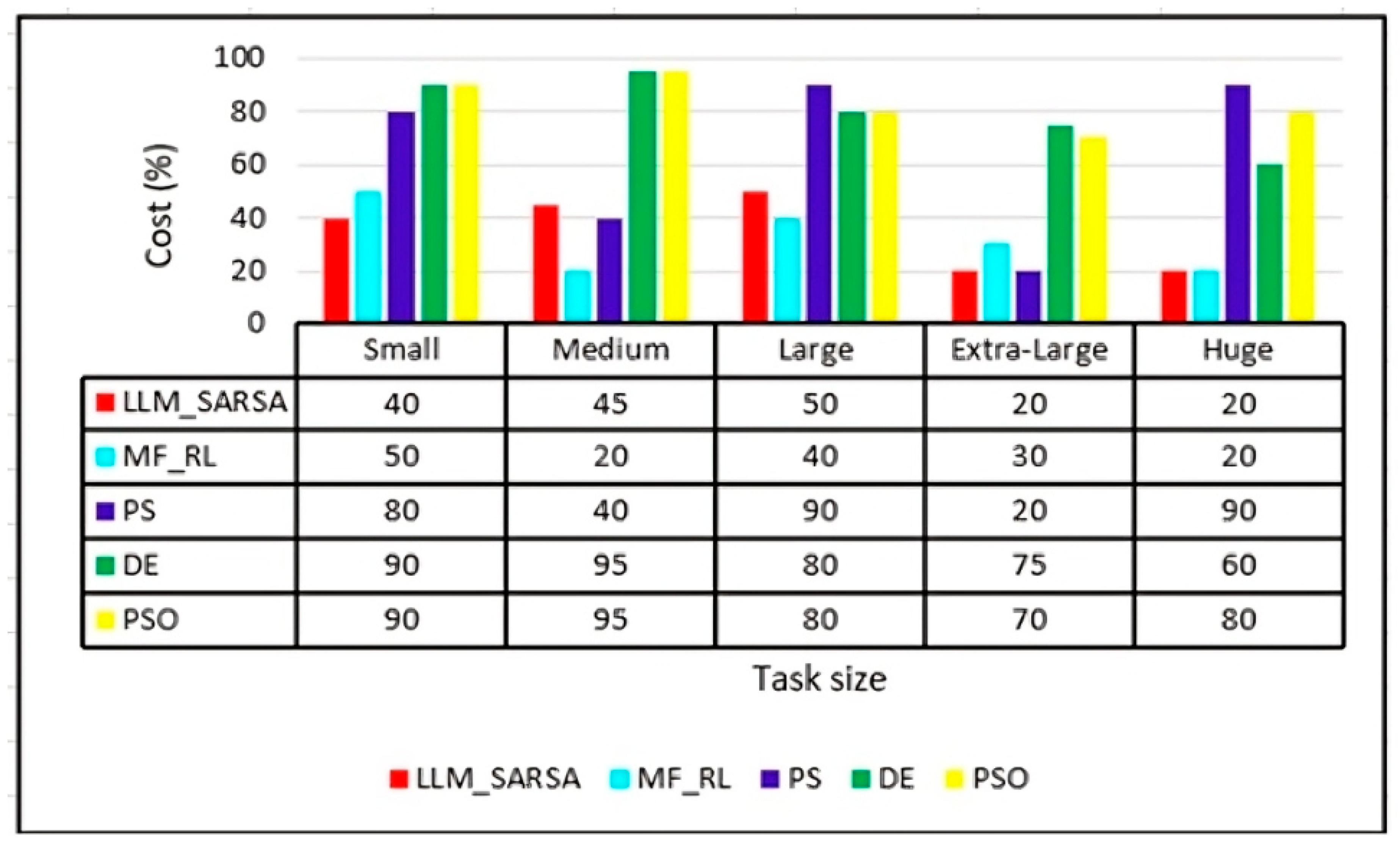
A graph of the Google clusters versus the degree of imbalance is shown in Figure 3. It is observed from the graph that the degree of imbalance is very low in Cluster-1 and it consistently remains lesser for all other clusters also as the LLM guides SARSA learning in reward shaping and also handles wrong heuristics using the decay factor. The degree of imbalance of PS and DE are moderate for all forms of Google cluster workloads as they easily become stuck in local optima and suffer from premature convergence, whereas the degree of imbalance of MF_RL and PSO is very high for all varying workload characteristics of the Google cluster as they require a lot of samples to learn the pattern and often suffer from overfitting problems.

6.3. PO3: Cost

A graph of the task size versus the cost incurred is shown in Figure 4. It is observed from the graph that the cost of operation of the LLM_SARSA is consistently less for varying sizes of the incoming tasks as they prevent the overestimation or underestimation of the SARSA Q function as it can dynamically adapt to different task sizes without tuning the hyperparameters. The cost of operation of MF_RL is found to be average for small to huge sizes of tasks as it does not use any model for learning, which increases the sampling complexity, whereas the cost of operation of PS, DE, and PSO is found to be higher for all task sizes from a small size to huge size As the possibility of ignoring lower-priority tasks is high when exposed to a higher-diversity computation space.

6.4. PO4: Resource Utilization

A graph of the task size versus the resource utilization is shown in Figure 5. It is observed from the graph that the resource utilization of the LLM_SARSA remained consistently high for all varying sizes of tasks as it performs unbiased training of SARSA learning agents and rejects inaccurate hallucination guidance. The resource utilization of PS and DE is found to be average for small to huge sizes of tasks as the chances of becoming trapped in local optimal solution are high due to high sensitivity towards outlier parameters, whereas the resource utilization of MF_RL and PSO is found to be consistently less for all task sizes from a small size to huge size as it does not find out the candidate solution within a predefined period due to a sluggish convergence rate.

7. Conclusions

This paper presents a novel LLM-guided SARSA task scheduler for cloud computing. The reward reshaping is performed using the heuristic value of the LLM model, which overcomes the inaccurate guidance problem. The constraint monitoring of the task scheduling response through zero-shot learning aids in effective operation even under uncertain cloud environments. The mathematical modeling of the task scheduler is conducted considering finite and infinite cloud scenarios. The experimental evaluation is carried out using the CloudSim 3.3 simulator. The practical results obtained are found to outperform four of the existing works with respect to the performance objectives: the makespan time, degree of imbalance, cost, and resource utilization. As extended work, exhaustive testing of the framework will be performed towards the following higher-end performance objectives: fault tolerance, correctness, confidentiality, reliability, and transparency.

References

1. Gunukula, S. The Future of Cloud Computing: Key Trends and Predictions for the Next Decade. Int. J. Res. Comput. Appl. Inf. Technol. 2024, 7, 528–538. [Google Scholar]
2. Wang, Y.; Bao, Q.; Wang, J.; Su, G.; Xu, X. Cloud computing for large-scale resource computation and storage in machine learning. J. Theory Pract. Eng. Sci. 2024, 4, 163–171. [Google Scholar] [CrossRef] [PubMed]
3. Soni, P.K.; Dhurwe, H. Challenges and Open Issues in Cloud Computing Services. In Advanced Computing Techniques for Optimization in Cloud; Chapman and Hall/CRC: New York, NK, USA, 2024; pp. 19–37. [Google Scholar]
4. Raja, V. Exploring challenges and solutions in cloud computing: A review of data security and privacy concerns. J. Artif. Intell. Gen. Sci. 2024, 4, 121–144. [Google Scholar]
5. Pramanik, S. Central Load Balancing Policy Over Virtual Machines on Cloud. In Balancing Automation and Human Interaction in Modern Marketing; IGI Global: Hershey, PA, USA, 2024; pp. 96–126. [Google Scholar]
6. Liu, Y.; Meng, Q.; Chen, K.; Shen, Z. Load-aware switch migration for controller load balancing in edge–cloud architectures. Future Gener. Comput. Syst. 2025, 162, 107489. [Google Scholar] [CrossRef]
7. Devi, N.; Dalal, S.; Solanki, K.; Dalal, S.; Lilhore, U.K.; Simaiya, S.; Nuristani, N. A systematic literature review for load balancing and task scheduling techniques in cloud computing. Artif. Intell. Rev. 2024, 57, 276. [Google Scholar] [CrossRef]
8. Patwari, K.R.; Kumar, R.; Sastry, J.S.V.R.S. A Systematic Review of Optimal Task Scheduling Methods Using Machine Learning in Cloud Computing Environments. In International Conference on Advances in Information Communication Technology & Computing; Springer Nature: Singapore, 2024; pp. 321–333. [Google Scholar]
9. Mehta, R.; Sahni, J.; Khanna, K. Task scheduling for improved response time of latency sensitive applications in fog integrated cloud environment. Multimed. Tools Appl. 2023, 82, 32305–32328. [Google Scholar] [CrossRef]
10. Jayanetti, A.; Halgamuge, S.; Buyya, R. Multi-agent deep reinforcement learning framework for renewable energy-aware workflow scheduling on distributed cloud data centres. IEEE Trans. Parallel Distrib. Syst. 2024, 35, 604–615. [Google Scholar] [CrossRef]
11. Arasan, K.K.; Anandhakumar, P. Energy-efficient task scheduling and resource management in a cloud environment using optimized hybrid technology. Softw. Pract. Exp. 2023, 53, 1572–1593. [Google Scholar] [CrossRef]
12. Zhang, S.; Wu, T.; Pan, M.; Zhang, C.; Yu, Y. A-SARSA: A predictive container auto-scaling algorithm based on reinforcement learning. In Proceedings of the 2020 IEEE International Conference on Web Services (ICWS), Beijing, China, 19–23 October 2020; pp. 489–497. [Google Scholar]
13. Zhai, Y.; Yang, T.; Xu, K.; Dawei, F.; Yang, C.; Ding, B.; Wang, H. Enhancing decision-making for llm agents via step-level q-value models. arXiv 2024, arXiv:2409.09345. [Google Scholar]
14. Wang, B.; Qu, Y.; Jiang, Y.; Shao, J.; Liu, C.; Yang, W.; Ji, X. LLM-empowered state representation for reinforcement learning. arXiv 2024, arXiv:2407.13237. [Google Scholar]
15. Zhang, S.; Zheng, S.; Ke, S.; Liu, Z.; Jin, W.; Yang, Y.; Yang, H.; Wang, Z. How Can LLM Guide RL? A Value-Based Approach. arXiv 2024, arXiv:2402.16181. [Google Scholar]
16. Prakash, B.; Oates, T.; Mohsenin, T. LLM Augmented Hierarchical Agents. arXiv 2023, arXiv:2311.05596. [Google Scholar]
17. Ni, W.; Zhang, Y.; Li, W. Optimal Dynamic Task Scheduling in Heterogeneous Cloud Computing Environment. In Proceedings of the 2024 IEEE International Conference on Industry 4.0, Artificial Intelligence, and Communications Technology (IAICT), BALI, Indonesia, 4–6 July 2024; pp. 40–46. [Google Scholar]
18. Sandhu, R.; Faiz, M.; Kaur, H.; Srivastava, A.; Narayan, V. Enhancement in performance of cloud computing task scheduling using optimization strategies. Clust. Comput. 2024, 27, 1–24. [Google Scholar] [CrossRef]
19. Wang, Y.; Dong, S.; Fan, W. Task scheduling mechanism based on reinforcement learning in cloud computing. Mathematics 2023, 11, 3364. [Google Scholar] [CrossRef]
20. Lipsa, S.; Dash, R.K.; Ivković, N.; Cengiz, K. Task scheduling in cloud computing: A priority-based heuristic approach. IEEE Access 2023, 11, 27111–27126. [Google Scholar] [CrossRef]
21. Abdel-Basset, M.; Mohamed, R.; Elkhalik, W.A.; Sharawi, M.; Sallam, K.M. Task scheduling approach in cloud computing environment using hybrid differential evolution. Mathematics 2022, 10, 4049. [Google Scholar] [CrossRef]
22. Nabi, S.; Ahmad, M.; Ibrahim, M.; Hamam, H. AdPSO: Adaptive PSO-based task scheduling approach for cloud computing. Sensors 2022, 22, 920. [Google Scholar] [CrossRef] [PubMed]
23. Habaebi, M.H.; Merrad, Y.; Islam, M.R.; Elsheikh, E.A.; Sliman, F.M.; Mesri, M. Extending CloudSim to simulate sensor networks. Simulation 2023, 99, 3–22. [Google Scholar] [CrossRef]
24. Hewage, T.B.; Ilager, S.; Rodriguez, M.A.; Buyya, R. CloudSim express: A novel framework for rapid low code simulation of cloud computing environments. Softw. Pract. Exp. 2024, 54, 483–500. [Google Scholar] [CrossRef]
Figure 1. The high-level architecture of LLM-guided SARSA task scheduler.
Mathematics 13 00926 g001
Figure 2. Google clusters versus makespan time (ms).
Mathematics 13 00926 g002
Figure 3. Google clusters versus degree of imbalance (0–1).
Mathematics 13 00926 g003
Figure 4. Task size versus cost incurred (%).
Mathematics 13 00926 g004
Figure 5. Task size versus resource utilization (%).
Mathematics 13 00926 g005