Efficient Scalar Multiplication of ECC Using Lookup Table and Fast Repeating Point Doubling

Abstract

Reducing the computation time of scalar multiplication for elliptic curve cryptography is a significant challenge. This study proposes an efficient scalar multiplication method for elliptic curves over finite fields $GF(2^m)$. The proposed method first converts the scalar into a binary number. Then, using Horner’s rule, the binary number is divided into fixed-length bit-words. Each bit-word undergoes repeating point doubling, which can be precomputed. However, repeating point doubling typically involves numerous inverse operations. To address this, significant effort has been made to develop formulas that minimize the number of inverse operations. With the proposed formula, regardless of how many times the operation is repeated, only a single inverse operation is required. Over $GF(2^m)$, the proposed method for scalar multiplication outperforms the sliding window method, which is currently regarded as the fastest available. However, the introduced formulas require more multiplications, squares, and additions. To reduce these operations, we further optimize the square operations; however, this introduces a trade-off between computation time and memory size. These challenges are key areas for future improvement.

1. Introduction

Elliptic curve cryptography (abbreviated as ECC) was introduced by Miller [1] in 1986 and Koblitz [2] in 1987. ECC is typically defined over prime finite fields $GF(p)$ or binary finite fields $GF(2^m)$. Public key cryptographic primitives can be implemented using abelian groups generated by elliptic curves over $GF(p)$ or $GF(2^m)$. ECC provides the same level of security as traditional public key cryptography, but with a smaller number of parameters. In practical applications, ECC over $GF(p)$ and $GF(2^m)$ each possess distinct advantages, and the choice between them depends on the specific requirements of the application. For example, $GF(p)$ is often preferred in scenarios demanding high security and versatility, such as financial transactions, digital signatures, and SSL/TLS protocols. ECC over $GF(p)$ generally provides stronger security guarantees and is well supported in both hardware and software implementations. On the other hand, $GF(2^m)$ is particularly suitable for resource-constrained environments, such as embedded systems and Internet of Things (IoT) devices, due to its computational efficiency. Operations over $GF(2^m)$ can be significantly accelerated through hardware optimization, making them more advantageous in scenarios where high computational efficiency is critical.

ECC designs over prime fields generally offer stronger resistance to side-channel attacks, while designs over binary fields benefit from a carry-free feature, making arithmetic operations more suitable for hardware implementation. ECC employs an encryption technique based on the discrete logarithm problem. The discrete logarithm problem is defined as follows: Given an elliptic curve E over a finite field and two points P and Q on E, the task is to find the value of k such that $Q=kP$. However, scalar multiplications and point inversions both are computationally intensive and represent key challenges. Regarding ECC defined over finite fields, numerous methods have been developed to optimize scalar multiplication and point inversion, including algebraic theorem-based designs [3], bit-slicing techniques [4], lookup tables [5], non-adjacent forms (NAFs) [6], and so on. For instance, the method in [7] minimizes the number of non-zero bits using the direct recoding method [8] to enhance scalar multiplication. Implementing ECC arithmetic operations on various coordinates can lead to faster computations. In [9], Jacobian coordinates are used to achieve high-efficiency point addition and doubling without requiring point inversions. In [10], the authors derive formulas for $3P$ in $\lambda$-projective coordinates and for $5P$ in both affine and $\lambda$-projective coordinates, marking the first study in $\lambda$-projective coordinates.

The methods presented in [11,12,13] transform scalar multiplication processes from affine to projective coordinate systems, with implementations verified on FPGA boards. For a more in-depth analysis on using various coordinates, we refer the reader to [14]. In terms of hardware implementations, the lookup table approach in [15] optimizes double point-doubling operations, while the triple-based chain method [16] reduces time consumption in elliptic curve cryptosystems. A low-latency window algorithm [17] enhances security, as does an enhanced comb method for point addition and doubling. In [18], a configurable ECC crypto-processor defined with the Weierstrass equation over prime fields was implemented and verified on a Xilinx FPGA board. Modular multipliers over $GF(2^m)$ are discussed in [19], and algorithmic improvements for computational complexity in low-power devices are presented in [20].

Reducing the number of inverse operations in scalar multiplication is crucial, as inversion over finite fields is the most time-consuming of all basic operations. In this work, a modified Horner’s rule based on binary scalar representation and a grouping technique are employed to accelerate scalar multiplication. Using the grouping technique, the scalar is partitioned into bit-words, where each represents a sum of repeating point doublings that can be precomputed and stored. Instead of traditional point doubling, this study derives formulas for performing repeating point doubling. These formulas require only one inversion operation regardless of the number of repetitions. Unlike projective coordinate systems, the derived formulas are based on the affine coordinate system. To the best of our knowledge, these formulas are the first to compute scalar multiplication in this manner. Additionally, the proposed method is suitable for both software and hardware implementations, as the arithmetic operations are simple and consistent in execution. From a software perspective, the proposed method achieves faster scalar multiplication computation compared with the sliding window algorithm [21]. While the sliding window method [21] is a highly efficient general-purpose technique and is widely regarded as the fastest available, it may not be optimal for all scenarios. Integrating the proposed method with the sliding window algorithm can further enhance its performance.

The contributions of this study are as follows:

• We propose an efficient repeating point-doubling algorithm that relies solely on standard inversion operations.
• A generalizable accelerated squaring method is introduced, which can be applied to inverse element computation.
• The proposed repeating point-doubling algorithm can enhance the performance of the sliding window method or any other technique requiring repeating point-doubling operations.
• The calculation of repeated point doubling is a critical component in algorithms for computing scalar multiplication. By replacing these operations with our proposed method, we can achieve further improvements in efficiency. For instance, our approach demonstrates significant performance gains when applied to techniques such as the sliding window algorithm, as evidenced by the experimental data presented in Section 4.

The rest of this paper is organized as follows: Section 2 introduces finite field arithmetic on elliptic curves. In Section 3, formulas for repeating point doubling are derived, which significantly reduce the computation time compared with traditional point doubling. Additionally, a modified square operation is introduced to further improve efficiency. Section 4 presents the results of the simulation implemented in Python 3.9 and executed on an Intel Core i9-14900K processor, showcasing the performance of the proposed methods. Finally, conclusions are provided in Section 5.

2. Preliminaries

2.1. Basic Operations on $GF(2^m)$

In the following, the binary operator “+” will denote an addition operation, which may vary depending on the context, such as addition of real numbers, bits, polynomials, or points on an elliptic curve. The exact meaning of “+” will be clear from the context in which it is used. When $a,b\in \{0,1\}$, the operation $a+b$ refers to the addition modulo 2 (i.e., binary addition).

Let $A=a_{m-1}{a}_{m-2}\dots a_1{a}_0$ be an element in $GF(2^m)$, where $a_i\in \{0,1\}$ for $0\le i\le m-1$. Then, A can be represented as a polynomial $A(x)={\sum }_{i=0}^{m-1}{a}_i{x}^i$. For simplicity, $A(x)$ is referred to as being defined over $GF(2^m)$. Let $B(x)={\sum }_{i=0}^{m-1}{b}_i{x}^i$ be defined over $GF(2^m)$. Then, the addition of $A(x)$ and $B(x)$, denoted as $A(x)+B(x)$, is defined by ${\sum }_{i=0}^{m-1}(a_i+b_i)x^i$. For example, suppose that $A=10101110$ and $B=11011011$ are elements in $GF(2^8)$. We can express these binary elements as polynomials $A(x)=x^7+x^5+x^3+x^2+x$ and $B(x)=x^7+x^6+x^4+x^3+x+1.$ Now, performing the addition $A(x)+B(x)$, which is equivalent to bitwise addition modulo 2, we obtain the following:

$$\begin{array}{c}\hfill \begin{array}{ccc}A(x)+B(x)\hfill & =\hfill & (1+1)x^7+(0+1)x^6+(1+0)x^5+(0+1)x^4+(1+1)x^3\hfill \\ & & +(1+0)x^2+(1+1)x+(0+1)\hfill \\ & =\hfill & x^6+x^5+x^4+x^2+1.\hfill \end{array}\end{array}$$

(1)

or equivalently, in binary form: $A+B=01110101.$ In programming, $(a_i+b_i)$ is the XOR operation of $a_i$ and $b_i$. The multiplication of $A(x)$ and $B(x)$ is the remainder $R(x)$ of the product of $A(x)$ and $B(x)$ by dividing an irreducible polynomial $f(x)$ of degree m defined over $GF(2^m)$. Symbolically, the multiplication of $A(x)$ and $B(x)$ in $GF(2^m)$ is denoted as $R(x)\equiv A(x)B(x)\mathbf{mod}f(x)$.

Over $GF(2^m)$, the Extended Euclidean Algorithm is employed to compute the remainder of the product of $A(x)$ and $B(x)$ by dividing $f(x)$. However, there are many time-consuming divisions in the algorithm. In order to avoid the divisions, Fermat’s Little Theorem is usually employed to compute the remainder or inverse. A polynomial $B(x)$ is said to be the inverse of a polynomial $A(x)$ if

$$A(x)B(x)\equiv \mathbf{mod}f(x).$$

We denote $B(x)$ as $A^{-1}(x)$. In Fermat’s Little Theorem, suppose that A is an element in $GF(2^m)$. Then, the inverse $A^{-1}$ of A is equal to $A^{2^m-2}$; moreover, $A^{2^m-2}={\prod }_{i=1}^{m-1}{A}^{2^i}$.

2.2. Point Addition and Point Doubling on Elliptic Curve

The elliptic curve $E(x,y)$ defined in $GF(2^m)$ is given by $y^2+xy=x^3+A{x}^2+B$, where A and B are elements in $GF(2^m)$. Let $P=(x_1,y_1)$ and $Q=(x_2,y_2)$ be two points in $E(x,y)$. The point addition of P and Q, denoted by $P+Q$, is the point $(x_3,y_3)$ in $E(x,y)$ obtained as follows:

• If $P\ne Q$, $P+Q$ is defined by the negative of the point that is the intersection of $E(x,y)$ and the line passing through P and Q. Let $\lambda$ denote the slope of the line. Then,

  $$\begin{array}{c}\hfill \lambda ={\displaystyle \frac{y_1+y_2}{x_1+x_2}}=(y_1+y_2){(x_1+x_2)}^{-1},x_3={\lambda }^2+\lambda +x_1+x_2+A,\mathrm{and}{y}_3=y_1+(x_1+x_3)\lambda +x_3.\end{array}$$
• If $P=Q$, $P+P$ is the negative of the point that is the intersection of $E(x,y)$ and the tangent line passing through the point P. $P+P$ is written as $2P=(x_2,y_2)$ and is called the point doubling of P, and we have

  $$\begin{array}{c}\hfill \lambda =x_1+{\displaystyle \frac{y_1}{x_1}}=x_1+y_1{x}_1^{-1},x_2={\lambda }^2+\lambda +A,\mathrm{and}{y}_2=x_1^2+(\lambda +1)x_2.\end{array}$$

  (2)

An illustrative example is presented based on the definitions of point addition and point doubling as follows. Over $GF(2^5)$, let $P=(x_1,y_1)=(00110,10000),Q=(x_2,y_2)=(01010,10010)$ be points on $y^2+xy=x^3+A{x}^2+B$, where $A=0001,B=0001$, and an irreducible polynomial $f(x)=x^5+x+1$. Let $R=(x_3,y_3)=P+Q$. Then,

$$\begin{array}{ccc}\lambda \hfill & =\hfill & {\displaystyle \frac{y_1+y_2}{x_1+x_2}}\hfill \\ & =\hfill & {\displaystyle \frac{10000+10010}{00110+01010}}\hfill \\ & =\hfill & {\displaystyle \frac{00010}{01100}}=(00010)(00111)=01110,\hfill \\ x_3\hfill & =\hfill & {\lambda }^2+\lambda +x_1+x_2+A\hfill \\ & =\hfill & {(01110)}^2+01110+00110+01010+00001=11101,\mathrm{and}\hfill \\ y_3\hfill & =\hfill & y_1+(x_1+x_3)\lambda +x_3\hfill \\ & =\hfill & 10000+(00110+11101)(01110)+11101=11011.\hfill \end{array}$$

Let $P+P=(x_2,y_2)$. Then,

$$\begin{array}{ccc}\lambda \hfill & =\hfill & x_1+{\displaystyle \frac{y_1}{x_1}}\hfill \\ \hfill & =\hfill & 00110+{\displaystyle \frac{10000}{00110}}\hfill \\ \hfill & =\hfill & 00110+(10000)(01110)=00110+11011=11101\hfill \\ x_2\hfill & =\hfill & {\lambda }^2+\lambda +A\hfill \\ \hfill & =\hfill & {(11101)}^2+11101+00001\hfill \\ \hfill & =\hfill & 10110+11101+00001=01010,\mathrm{and}\hfill \\ y_2\hfill & =\hfill & x_1^2+(\lambda +1)x_2\hfill \\ \hfill & =\hfill & {(00110)}^2+(11101+00001)(01010)\hfill \\ \hfill & =\hfill & 10100+00110=10010.\hfill \end{array}$$

3. Optimizing Scalar Multiplications

3.1. Scalar Multiplication

Let $k\ge 2$ be an integer and P be a point in $E(x,y):y^2+xy=x^3+A{x}^2+B$. The scalar multiplication $kP$ of P is defined by $kP=\underset{k}{\underbrace{P+P+\cdots +P}}$. The computation of $kP$ is lengthy. To reduce the duration, first, k is converted to a binary representation, as follows:

$$\begin{array}{c}\hfill k_{m-1}{2}^{m-1}+k_{m-2}{2}^{m-2}+\cdots +k_1{2}^1+k_0{2}^0,\end{array}$$

(3)

where $k_i\in \{0,1\}$ for $0\le i\le m-1$. Let $d,w,r$ be non-negative integers such that $m=w·d+r$ with $0\le r\le w-1$. Then, using Horner’s rule, Equation (3) can be represented as

$$\begin{array}{ccc}k\hfill & =\hfill & \underset{d}{\underbrace{((\cdots (}}{k}_{m-1}{2}^{w-1}+k_{m-2}{2}^{w-2}+\cdots +k_{m-(w-1)}2+k_{m-w})2^w\hfill \\ & +\hfill & k_{m-w-1}{2}^{w-1}+k_{m-w-2}{2}^{w-2}+\cdots +k_{m-w-(w-1)}2+k_{m-w-w})2^w+\cdots \hfill \\ \\ & +\hfill & k_{m-(d-1)w-1}{2}^{w-1}+k_{m-(d-1)w-2}{2}^{w-2}+\cdots +k_{m-(d-1)w-(w-1)}2+k_{m-(d-1)w-w})2^r\hfill \\ \\ & +\hfill & k_{r-1}{2}^{r-1}+k_{r-2}{2}^{r-2}+\cdots k_{1}2+k_0.\hfill \end{array}$$

For example, suppose that $k=2^{14}+2^{12}+2^{11}+2^9+2^8+2^6+2^5+2^4+2+1$ and $w=3$. Then,

$$\begin{array}{c}\hfill \begin{array}{ccc}k\hfill & =& ((((2^2+0·2^1+2^0)2^3+2^2+0·2^1+2^0)2^3+2^2+0·2^1+2^0)2^3\hfill \\ & & +2^2+2^1+0·2^0)2^3+0·2^2+2^1+2^0.\hfill \end{array}\end{array}$$

(4)

As the idea behind the proposed method comes from the sliding window [21], let us briefly introduce the basic concept of the sliding window by the following example. For k in Equation (4) with window size $w=3$, k can be written as

$$\begin{array}{c}\hfill k=101101101110011.\end{array}$$

(5)

In accordance with the sliding window method, the precomputations are $(\lceil 15/3\rceil -1)$ point additions; a point doubling number of 9; and $2P$, $3P(2P+P)$, $5P(3P+2P)$, and $7P(5P+2P)$. The number of point doubling is the number of times a window with length w is successively shifted one place from left to right, skipping the zeros if they are not in the window. More details on the sliding window method can be found in [21]. With the proposed method, $kP$ is written as

$$\begin{array}{c}\hfill \begin{array}{ccc}kP\hfill & =\hfill & \underset{d}{\underbrace{((\cdots (}}{k}_{m-1}{2}^{w-1}P+k_{m-2}{2}^{w-2}P+\cdots +k_{m-(w-1)}2P+k_{m-w}P)2^w\hfill \\ & +\hfill & k_{m-w-1}{2}^{w-1}P+k_{m-w-2}{2}^{w-2}P+\cdots +k_{m-w-(w-1)}2P+k_{m-w-w}P)2^w\hfill \\ & +\hfill & \cdots \hfill \\ & +\hfill & k_{m-(d-1)w-1}{2}^{w-1}P+k_{m-(d-1)w-2}{2}^{w-2}P+\cdots \hfill \\ & & +k_{m-(d-1)w-(w-1)}2P+k_{m-(d-1)w-w}P)2^r\hfill \\ & +\hfill & k_{r-1}{2}^{r-1}P+k_{r-2}{2}^{r-2}P+\cdots k_{1}2P+k_{0}P.\hfill \end{array}\end{array}$$

(6)

In Equation (6), for $0\le i\le d-1$, each

$$\begin{array}{c}\hfill k_{m-iw-1}{2}^{w-1}P+k_{m-iw-2}{2}^{w-2}P+\cdots +k_{m-iw-(w-1)}2P+k_{m-iw-w}P\end{array}$$

(7)

is referred to as a w-bit word, denoted as $(k_{w-1}^i,k_{w-2}^i,\cdots ,k_1^i,k_0^i)$. For the last r terms,

$$\begin{array}{c}\hfill k_{r-1}{2}^{r-1}P+k_{r-2}{2}^{r-2}P+\cdots +k_{1}2P+k_{0}P\end{array}$$

(8)

in Equation (6) is also represented as a w-bit word $(k_{w-1}^d,k_{w-2}^d,\cdots ,k_r^d,k_{r-1}^d,k_{r-2}^d,\cdots ,k_1^d,k_0^d)$ with $k_j^d=0$ for $r\le j\le w-1$.

For Equations (7) and (8), it is evident that any scalar multiplication operation can be equivalently expressed as the computation of $2P,2^{2}P,\cdots$, $2^{w-1}P$ for each i. For a small value of w, the points $2P,2^{2}P,\cdots ,(2^w-1)P$ can be precomputed and stored in advance, as illustrated in

Table 1. Precomputations for Equations (7) and (8).

$\mathit{L}({\mathit{k}}_{\mathit{m}-\mathit{iw}+\mathit{w}-1},{\mathit{k}}_{\mathit{m}-\mathit{iw}+\mathit{w}-2},\cdots ,{\mathit{k}}_{\mathit{m}-\mathit{iw}+\mathit{w}-(\mathit{w}-1)},{\mathit{k}}_{\mathit{m}-\mathit{iw}+\mathit{w}-\mathit{w}})$	${\sum }_{\mathit{j}=0}^{\mathit{w}-1}{\mathit{k}}_{\mathit{m}-\mathit{iw}-(\mathit{w}-\mathit{j})}{2}^{\mathit{j}}\mathit{P}$
$L(0,0,0,\cdots ,0,0,0)$	0
$L(0,0,0,\cdots ,0,0,1)$	P
$L(0,0,0,\cdots ,0,1,0)$	$2P$
$L(0,0,0,\cdots ,0,1,1)$	$L(0,0,0,\cdots ,0,0,1)+L(0,0,0,\cdots ,0,1,0)=3P$
$L(0,0,0,\cdots ,1,0,0)$	$2^{2}P$
⋮	⋮
$L(1,0,0,\cdots ,0,0,0)$	$2^{w-1}P$
$L(1,0,0,\cdots ,0,0,1)$	$L(1,0,0,\cdots ,0,0,0)+L(0,0,0,\cdots ,0,0,1)=2^{w-1}P+P$
⋮	⋮
$L(1,1,1,\cdots ,1,1,1)$	$L(1,0,0,\cdots ,0,0,0)+L(0,1,1,\cdots ,1,1,1)=(2^w-1)P$

. In this table, given the point P, the scalar k, and the word length w, the result of Equation (7) or (8) can be directly retrieved from the entry $L(k_{m-iw+w-1},k_{m-iw+w-2},\cdots ,k_{m-iw+w-(w-1)},k_{m-iw+w-w})$, provided that $k_j^i=k_{m-iw+j}$ for $0\le i\le d$ and $0\le j\le w-1$.

We will use the following example to demonstrate how to look up values in Table 1. Suppose that $w=3$; we precompute all eight possible combinations, as shown in the following table. For the value of k according to Equation (5), for the combination 110, we obtain the result from the table entry $L(1,1,0)$, which is $6P$.

$L(k_2,k_1,k_0)$	$k_2{P}^2+k_{1}P+k_{0}P$
$L(0,0,0)$	0
$L(0,0,1)$	P
$L(0,1,0)$	$2P$
$L(0,1,1)$	$2P+P$
$L(1,0,0)$	$4P$
$L(1,0,1)$	$4P+P$
$L(1,1,0)$	$4P+2P$
$L(1,1,1)$	$4P+3P$

Therefore, given point P, scalar k, and word length w, $kP$ can be computed with the following Algorithm 1, ScalarMUL.

Algorithm 1 ScalarMUL$(k,P,w)$
1.	Set  $Q=0$
2.	Using P to create table L, as shown in Table 1
3.	Set  $d=\lfloor m/w\rfloor$  and  $r=m-w·d$
4.	For $i\leftarrow d-1$ downto 0
5.	do
6.	$Q\leftarrow Q+L(k_{m-iw+w-1},k_{m-iw+w-2},\cdots ,k_{m-iw+w-(w-1)},k_{m-iw+w-w})$
7.	$Q\leftarrow 2^{w}Q$
8.	Enddo
9.	$Q\leftarrow 2^{r}Q$
10.	$Q\leftarrow Q+L(0,0,\cdots ,0,k_{r-1},k_{r-2},\cdots ,k_1,k_0)$
11.	return Q

3.2. Reducing Inverse in the Repeating Point Doubling

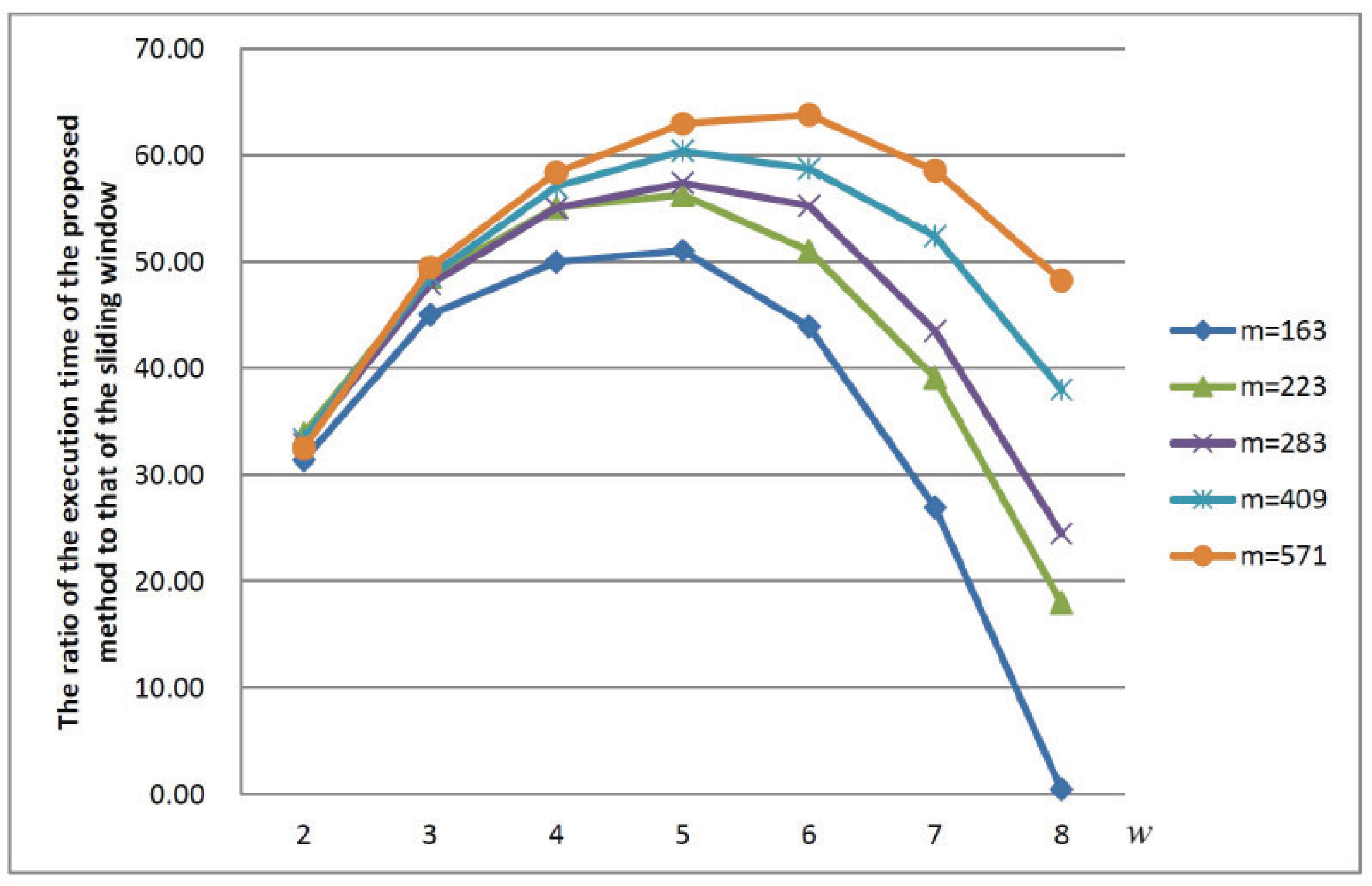
The sliding window method [21] shifts a window of length $w>0$ and skips over runs of zeros between them while disregarding the fixed digit boundaries. However, in the ScalarMUL algorithm, the binary representation of k is partitioned into fixed-length bit-words of size w, where each word is processed sequentially. This approach can also be extended to the sliding window method, as will be demonstrated in Section 4 with the experimental results. Within the ScalarMUL algorithm, it is necessary to compute $2^{w}Q$ in step 7 and $2^{r}Q$ in step 9.

According to the definition of scalar multiplication $kQ$ of Q and the associative property of point addition on the elliptic curve $E(x,y)$, for any positive integer n, $2^{n}Q$ can be expressed as the point doubling of $2^{n-1}Q$. Specifically, $2^{n}Q=2^{n-1}Q+2^{n-1}Q=2(2^{n-1}Q)$. Traditionally, as described in Equation (2), $2^{n}Q$ can be computed using the following Algorithm 2, referred to as Tradition. In the Tradition algorithm, line 4 employs Equation (2) to compute $2Q$. Each iteration performs a point-doubling operation on Q requiring five XORs (additions), two multiplications, and one inverse operation. The addition, multiplication, and square operations mentioned here are all operations defined within $GF(2^m)$.

Algorithm 2 Tradition$(n,P)$
1.	Set  $Q=P$
2.	For $i\leftarrow n-1$ downto 0
3.	do
4.	$Q\leftarrow 2Q$
5.	Enddo
6.	return  Q

To obtain $2^{n}Q$, we have to compute $2Q(Q+Q),4Q(2Q+2Q),\cdots ,2^n(2^{n-1}Q+2^{n-1}Q)$. Therefore, in the computation, there are n inverse operations, $5n$ XORs, $2n$ multiplications, and $2n$ squares. Since the inverse operation is computationally expensive, we have developed optimized formulas to replace the point-doubling computation in the Tradition algorithm. The derived formulas are designed to ensure that only a single inverse operation is required when computing $2^{n}Q$ of a given point Q, significantly improving computational efficiency. Let $Q_0=(x_0,y_0)$ be a point in $E(x,y)$. For $n\ge 1$, let $Q_n=(x_n,y_n)$ be the point doubling of $Q_{n-1}$. Then, $Q_n$ is the scalar multiplication $2^n{Q}_0$ of $Q_0$. Let ${\lambda }_n$ be the slope of the tangent line passing through the point $Q_{n-1}$. Then, to derive formulas for $Q_n$ obtained from $Q_0$ via the iteration of point doubling, first, consider $Q_1=(x_1,y_1)$. We have

$$\begin{array}{c}\hfill \begin{array}{ccc}{\lambda }_1\hfill & =\hfill & x_0+{\displaystyle \frac{y_0}{x_0}}={\displaystyle \frac{x_0^2+y_0}{x_0}}={\displaystyle \frac{v_1}{x_0}},\hfill \\ x_1\hfill & =\hfill & {\lambda }_1^2+{\lambda }_1+A={\left({\displaystyle \frac{v_1}{x_0}}\right)}^2+{\displaystyle \frac{v_1}{x_0}}+A={\displaystyle \frac{A{x}_0^2+v_1{x}_0+v_1^2}{x_0^2}}={\displaystyle \frac{u_1}{x_0^2}},\mathrm{and}\hfill \\ y_1\hfill & =\hfill & x_0^2+({\lambda }_1+1)x_1,\hfill \end{array}\end{array}$$

(9)

where $v_1=x_0^2+y_0$ and $u_1=A{x}_0^2+v_1{x}_0+v_1^2$.

In what follows, the formula for $y_n$ will be omitted until ${\lambda }_n$ and $x_n$ are obtained.

For $Q_2=2Q_1=(x_2,y_2)$,

$$\begin{array}{c}\hfill \begin{array}{ccc}{\lambda }_2\hfill & =\hfill & x_1+{\displaystyle \frac{y_1}{x_1}}={\lambda }_1^2+(A+1)+{\displaystyle \frac{x_0^2}{x_1}}={\displaystyle \frac{v_1^2}{x_0^2}}+(A+1)+{\displaystyle \frac{x_0^2{x}_0^2}{u_1}},\hfill \\ & =\hfill & {\displaystyle \frac{(A+1)u_1{x}_0^2+u_1{v}_1^2+x_0^2{(x_0^2)}^2}{u_1{x}_0^2}}={\displaystyle \frac{v_2}{u_1{x}_0^2}}\mathrm{and}\hfill \\ x_2\hfill & =\hfill & {\lambda }_2^2+{\lambda }_2+A={\displaystyle \frac{v_2^2}{{(u_1{x}_0^2)}^2}}+{\displaystyle \frac{v_2}{u_1{x}_0^2}}+A={\displaystyle \frac{A{(u_1{x}_0^2)}^2+v_2(u_1{x}_0^2)+v_2^2}{{(u_1{x}_0^2)}^2}}={\displaystyle \frac{u_2}{{(u_1{x}_0^2)}^2}},\hfill \end{array}\end{array}$$

(10)

where $v_2=(A+1)u_1{x}_0^2+u_1{v}_1^2+x_0^2{(x_0^2)}^2$ and $u_2=A{(u_1{x}_0^2)}^2+v_2(u_1{x}_0^2)+v_2^2$.

For $Q_3=2Q_2=(x_3,y_3)$,

$$\begin{array}{c}\hfill \begin{array}{ccc}{\lambda }_3\hfill & =\hfill & x_2+{\displaystyle \frac{y_2}{x_2}}={\lambda }_2^2+(A+1)+{\displaystyle \frac{x_1^2}{x_2}}\hfill \\ & =\hfill & {\displaystyle \frac{v_2^2}{{(u_1{x}_0^2)}^2}}+(A+1)+{\displaystyle \frac{u_1^2/x_0^4}{{(u_2/u_1{x}_0^2)}^2}}\hfill \\ & =\hfill & {\displaystyle \frac{(A+1)u_2{(u_1{x}_0^2)}^2+u_2{v}_2^2+{(u_1^2)}^2{(u_1{x}_0^2)}^2}{u_2{(u_1{x}_0^2)}^2}}={\displaystyle \frac{v_3}{u_2{(u_1{x}_0^2)}^2}}\mathrm{and}\hfill \\ x_3\hfill & =\hfill & {\lambda }_3^2+{\lambda }_3+A={\displaystyle \frac{v_3^2}{{(u_2{(u_1{x}_0^2)}^2)}^2}}+{\displaystyle \frac{v_3}{u_2{(u_1{x}_0^2)}^2}}+A\hfill \\ & =\hfill & {\displaystyle \frac{A{(u_2{(u_1{x}_0^2)}^2)}^2+v_3(u_2{(u_1{x}_0^2)}^2)+v_3^2}{{(u_2{(u_1{x}_0^2)}^2)}^2}}={\displaystyle \frac{u_3}{{(u_2{(u_1{x}_0^2)}^2)}^2}},\hfill \end{array}\end{array}$$

(11)

where $v_3=(A+1)u_2{(u_1{x}_0^2)}^2+u_2{v}_2^2+{(u_1^2)}^2{(u_1{x}_0^2)}^2$ and $u_3=A{(u_2{(u_1{x}_0^2)}^2)}^2+v_3(u_2{(u_1{x}_0^2)}^2)+v_3^2$.

For $Q_4=2Q_3=(x_4,y_4)$,

$$\begin{array}{c}\hfill \begin{array}{ccc}{\lambda }_4\hfill & =\hfill & x_3+{\displaystyle \frac{y_3}{x_3}}={\lambda }_3^2+(A+1)+{\displaystyle \frac{x_2^2}{x_3}}\hfill \\ & =\hfill & {\displaystyle \frac{v_3^2}{{(u_2{(u_1{x}_0^2)}^2)}^2}}+(A+1)+{\displaystyle \frac{u_2^2/{({(u_1{x}_0^2)}^2)}^2}{(u_3/{(u_2{(u_1{x}_0^2)}^2)}^2}}\hfill \\ & =\hfill & {\displaystyle \frac{(A+1)u_3{(u_2{(u_1{x}_0^2)}^2)}^2+u_3{v}_3^2+{(u_2^2)}^2{(u_2{(u_1{x}_0^2)}^2)}^2}{u_3{(u_2{(u_1{x}_0^2)}^2)}^2}}={\displaystyle \frac{v_4}{u_3{(u_2{(u_1{x}_0^2)}^2)}^2}}\mathrm{and}\hfill \\ x_4\hfill & =\hfill & {\lambda }_4^2+{\lambda }_4+A={\displaystyle \frac{v_4^2}{{(u_3{(u_2{(u_1{x}_0^2)}^2)}^2)}^2}}+{\displaystyle \frac{v_4}{u_3{(u_2{(u_1{x}_0^2)}^2)}^2}}+A\hfill \\ & =\hfill & {\displaystyle \frac{A{(u_3{(u_2{(u_1{x}_0^2)}^2)}^2)}^2+v_4(u_3{(u_2{(u_1{x}_0^2)}^2)}^2)+v_4^2}{{(u_3{(u_2{(u_1{x}_0^2)}^2)}^2)}^2}}={\displaystyle \frac{u_4}{{(u_3{(u_2{(u_1{x}_0^2)}^2)}^2)}^2}},\hfill \end{array}\end{array}$$

(12)

where

$$v_4=(A+1)u_3{(u_2{(u_1{x}_0^2)}^2)}^2+u_3{v}_3^2+{(u_2^2)}^2{(u_2{(u_1{x}_0^2)}^2)}^2$$

and

$$u_4=A{(u_3{(u_2{(u_1{x}_0^2)}^2)}^2)}^2+v_4(u_3{(u_2{(u_1{x}_0^2)}^2)}^2)+v_4^2.$$

The formulas for $x_n$ and ${\lambda }_n$ can be extended iteratively for arbitrarily large values of n, allowing us to compute $2^{n}Q$ for any desired n. However, the derivation process becomes increasingly laborious and cumbersome as n grows larger, making it impractical for manual computation. Before establishing that there is only one inverse operation involved in the computation of scalar multiplication, it will be helpful to introduce the following recurrence relations. By following Equations (9)–(12), let $t_1=x_0,t_2=u_1{x}_0^2$, and $t_3=u_2{(u_1{x}_0^2)}^2$. Then,

$$\begin{array}{c}\hfill v_3=(A+1)t_3+u_2{v}_2^2+{(u_1^2)}^2{t}_2^2\mathrm{and}{u}_3=A{t}_3^2+v_3{t}_3+v_3^2\end{array}$$

(13)

For $n\ge 3$, the following relationships can be easily derived:

$$\begin{array}{ccc}{t}_n\hfill & =\hfill & u_{n-1}{t}_{n-1}^2,\hfill \\ v_n\hfill & =\hfill & (A+1)t_n+u_{n-1}{v}_{n-1}^2+{(u_{n-2}^2)}^2{t}_{n-1}^2,\mathrm{and}\hfill \\ u_n\hfill & =\hfill & A{t}_n^2+v_n{t}_n+v_n^2.\hfill \end{array}$$

Table 2. Computations of ${\lambda }_4$ and $x_4$ for four times point doubling of $Q_0$ for $m=163$.

$A=$ 0x1, primitive polynomial $f(x)=x^{163}+x^7+x^6+x^3+1$, $Q_0=(x_0,y_0)$
$x_0=$ 0x02FE13C0537BBC11ACAA07D793DE4E6D5E5C94EEE8
$y_0=$ 0x0289070FB05D38FF58321F2E800536D538CCDAA3D9
$t_1=x_0$	0x2FE13C0537BBC11ACAA07D793DE4E6D5E5C94EEE8
$v_1=t_1^2+y_0$	0x4F80CD7EF766D64506FDDADAE0D599F74B2227367
$u_1=A{t}_1^2+v_1{t}_1+v_1^2$	0x32FBC2266652998D2D2F03AFD6241F309DDE4AE1B
$t_2=u_1{t}_1^2$	0x5A40058EDE40D0A67D4BD8CB03557EEC05F034063
$v_2=(A+1)t_2^2+u_1{v}_1^2+{(x_0^2)}^2{t}_1^2$	0x2792546E8CB0EE4CC70AB686063CA9C9EABCE3A12
$u_2=A{t}_2^2+v_2{t}_2+v_2^2$	0x52D96F1338F1AA0962CBCED0BF145D810E7F7E174
$t_3=u_2{t}^2$	0x17EA26AC56E2A438890799BFBDF518C44B1769326
$v_3=(A+1)t_3^2+u_2{v}_2^2+{(u_1^2)}^2{t}_2^2$	0x1A26B8B369A2A6FE9FE00452B82B49FFE32453AC
$u_3=A{t}_3^2+v_3{t}_3+v_3^2$	0x1415E6A7EE1563767A757312679BA44FCFA9C42DF
$t_4=u_3{t}_3^2$	0x2B4B1B80260F6CA1D0BE900A98486B175408B673D
$v_4=(A+1)t_4^2+u_3{v}_3^2{(u_2^2)}^2{t}_3^2$	0x79C9EAD3F5B5A625DF7C1D6E3F3C572181F7128E7
$u_4=A{t}_4^2+v_4{t}_4+v_4^2$	0x5DB8FC493F7495E19777B26FAF97457756AD27E2E
$t=t_4^{-1}$	0x145E47AFC3228B6070CCC6D1F3B9D178EA838006E
${\lambda }_4=v_{4}t$	0x7FDE58E3AE8F043ECDE437CA1581911B725743721
$x_4=u_4{t}^2$	0x2E8D15536960EB926E78D9E15CE721DFAE4FE3134

is an illustration of Equations (9)–(12) to compute ${\lambda }_4$ and $x_4$. In the example, the curve is defined over $GF(2^{163})$. For $m=233,283,409,571$, the computations of ${\lambda }_4$ and $x_4$ are shown in Appendix A.

Lemma 1.

For $n\ge 3$, ${\lambda }_n={\displaystyle \frac{v_n}{t_n}}$ and $x_n={\displaystyle \frac{u_n}{t_n^2}}$.

Proof of Lemma 1.

We will proceed with induction on n. Equations (9)–(12) show the basis step for ${\lambda }_n$ and $x_n$. For the inductive step,

$$\begin{array}{c}\hfill \begin{array}{ccc}{\lambda }_n\hfill & =\hfill & {\lambda }_{n-1}^2+(A+1)+{\displaystyle \frac{x_{n-2}^2}{x_{n-1}}}\hfill \\ & =\hfill & {\left({\displaystyle \frac{v_{n-1}}{t_{n-1}}}\right)}^2+(A+1)+{\displaystyle \frac{{\left(u_{n-2}/t_{n-2}^2\right)}^2}{u_{n-1}/t_{n-1}^2}}\hfill \\ & =\hfill & {\displaystyle \frac{v_{n-1}^2}{t_{n-1}^2}}+(A+1)+{\displaystyle \frac{u_{n-2}^2{t}_{n-1}^2}{u_{n-1}{t}_{n-2}^4}}\hfill \\ & =\hfill & {\displaystyle \frac{v_{n-1}^2}{t_{n-1}^2}}+(A+1)+{\displaystyle \frac{{(u_{n-2}^2)}^2}{u_{n-1}}}\hfill \\ & =\hfill & {\displaystyle \frac{(A+1)u_{n-1}{t}_{n-1}^2+u_{n-1}{v}_{n-1}^2+{(u_{n-2}^2)}^2{t}_{n-1}^2}{u_{n-1}{t}_{n-1}^2}}={\displaystyle \frac{v_n}{t_n}}\mathrm{and}\hfill \\ x_n\hfill & =\hfill & {\lambda }_n^2+{\lambda }_n+A={\left({\displaystyle \frac{v_n}{t_n}}\right)}^2+{\displaystyle \frac{v_n}{t_n}}+A={\displaystyle \frac{A{t}_n^2+v_n{t}_n+v_n^2}{t_n^2}}={\displaystyle \frac{u_n}{t_n^2}}.\hfill \end{array}\end{array}$$

(14)

This lemma holds.    □

Corollary 1.

For $n\ge 3$, $y_n={\displaystyle \frac{u_{n-1}^2{u}_{n-1}^2+({\lambda }_n+1)u_n}{t_n^2}}$.

Proof of Corollary 1.

According to Lemma 1, ${\lambda }_n={\displaystyle \frac{v_n}{t_n^2}}·t_n$,

$$\begin{array}{ccc}\hfill y_n& =& x_{n-1}^2+({\lambda }_n+1)x_n={\left({\displaystyle \frac{u_{n-1}}{t_{n-1}^2}}\right)}^2+({\lambda }_n+1){\displaystyle \frac{u_n}{t_n^2}}\hfill \\ & =& {\displaystyle \frac{u_{n-1}^2}{t_{n-1}^4}}+({\lambda }_n+1){\displaystyle \frac{u_n}{{(u_{n-1}{t}_{n-1}^2)}^2}}={\displaystyle \frac{u_{n-1}^2{u}_{n-1}^2+({\lambda }_n+1)u_n}{{(u_{n-1}{t}_{n-1}^2)}^2}}\hfill \\ & =& {\displaystyle \frac{u_{n-1}^2{u}_{n-1}^2+({\lambda }_n+1)u_n}{t_n^2}}.\hfill \end{array}$$

   □

Given a point $Q=(x,y)$ and a positive integer n, the n-times point doubling $2^{n}Q$ of Q can be efficiently computed using the following Algorithm 3, referred to as PDNTimes.

Algorithm 3 PDNTimes$(Q=(x,y),n)$
1.	Set  $Q_1=(0,0)$
2.	If $x\ne 0$, then
3.	$x_0\leftarrow x$; $y_0\leftarrow y$
4.	$u_0\leftarrow x_0$; $t_1\leftarrow x_0$
5.	$v_1\leftarrow t_1^2+y_0$
6.	$u_1\leftarrow A·t_1^2+v_1·t_1+v_1^2$
7.	For $i\leftarrow 2$ upto n
8.	do
9.	$t_i\leftarrow u_{i-1}·t_{i-1}^2$
10.	$v_i\leftarrow (A+1)·t_i+u_{i-1}·v_{i-1}^2+{(u_{i-2}^2)}^2·t_{i-1}^2$
11.	$u_i\leftarrow A·t_i^2+v_i·t_i+v_i^2$
12.	Enddo
13.	$t\leftarrow t_n^{-1}$
14.	${\lambda }_n\leftarrow v_n·t$
15.	$t^{\prime }\leftarrow t^2$
16.	$x_n\leftarrow u_n·t^{\prime }$
17.	$y_n\leftarrow ({(u_{n-1}^2)}^2+({\lambda }_n+1)·u_n)·t^{\prime }$
18.	$Q_1\leftarrow (x_n,y_n)$
19.	EndIf
20.	return  $Q_1$

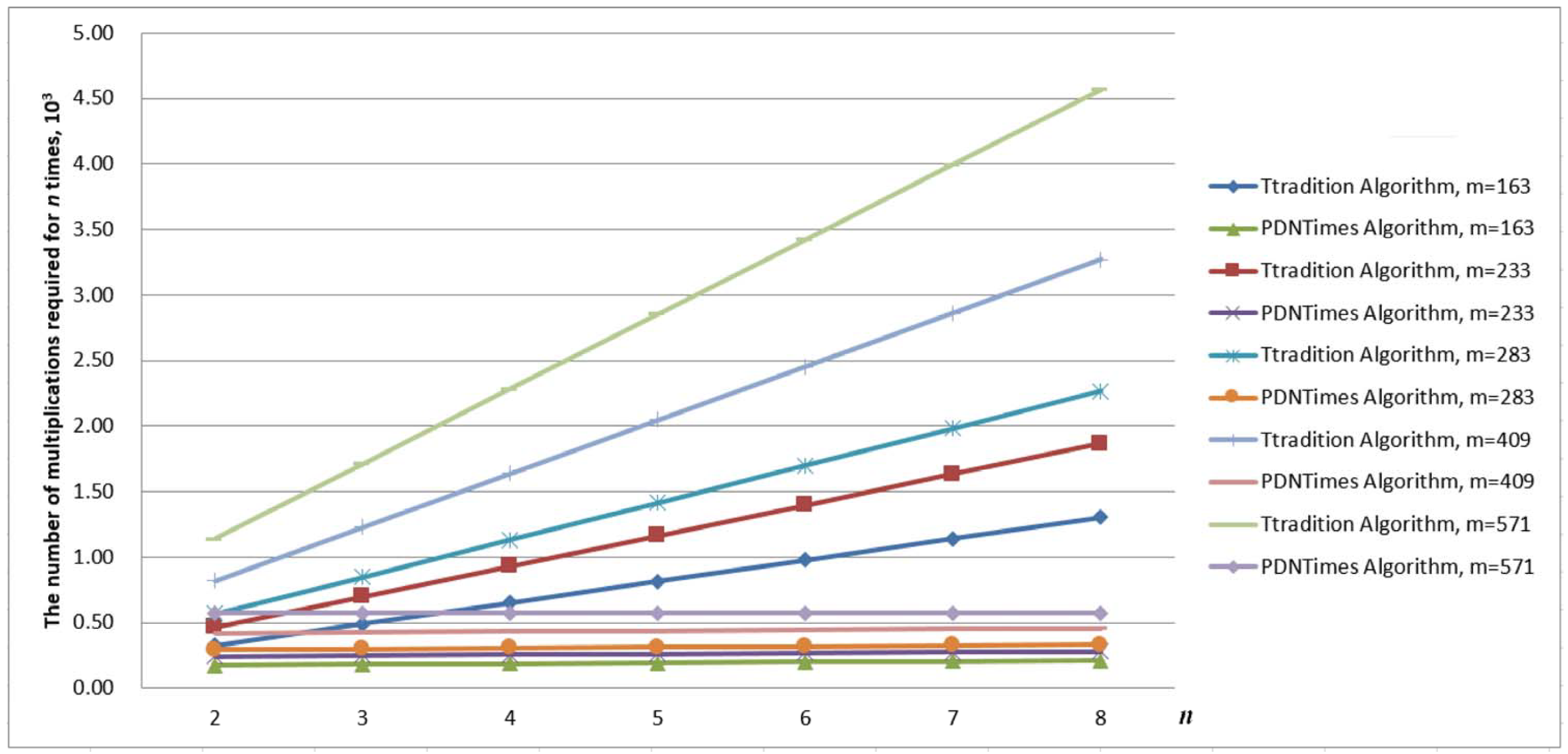
In the PDNTimes algorithm, the computational complexity can be broken down as follows:

• Lines 5 and 6: These lines involve 3 XOR operations, 2 multiplications, and 2 square operations.
• Lines 9–11: Each iteration of the loop in these lines requires 5 XOR operations, 6 multiplications, and 6 square operations.
• Lines 13–17: These lines consist of 2 XOR operations, 4 multiplications, 3 square operations, and 1 inverse operation.

Therefore, a total of $5n$ XORs, $6n$ multiplications, and $6n-1$ squares are required. However, in the case of hardware devices, the time complexity of adding any two n-bit numbers is currently $O(1)$, while the time complexity of their multiplication is $O(n)$.

Lemma 2.

Over $GF(2^m)$, let $n\ge 2$ be an integer and Q be a point in $E(x,y):y^2+xy=x^3+A{x}^2+B$. The computation of n times point doubling $2^{n}Q$ of Q requires $O(n)$ multiplications, $O(n)$ squares, and one inverse operation.

For the repeating point doubling on $GF(2^m)$,

Table 3. The execution times (${10}^{-3}$ s) for Tradition and PDNTimes over $GF(2^m)$ and the decreasing ratio, where $m=163,233,283,409,571$.

m	Method	n
	Ratio	2	3	4	5	6	7	8
163	Tradition	11.024	17.369	25.359	31.436	36.060	41.873	48.851
	PDNTimes	6.217	6.462	6.641	6.762	7.034	7.205	7.319
	ratio	43.60	62.80	73.81	78.49	80.49	82.79	85.02
233	Tradition	24.701	37.534	50.078	61.188	73.936	89.568	99.046
	PDNTimes	12.859	13.195	13.374	13.557	14.197	14.222	14.541
	ratio	47.94	64.85	73.29	77.84	80.80	84.12	85.32
283	Tradition	39.671	62.621	79.533	103.221	123.985	144.111	163.431
	PDNTimes	20.762	21.181	21.731	21.733	22.341	22.653	23.138
	ratio	47.66	66.18	72.68	78.95	81.98	84.28	85.84
409	Tradition	88.431	132.481	176.825	218.813	262.292	306.032	349.894
	PDNTimes	44.307	45.134	45.792	46.015	46.691	47.969	48.554
	ratio	49.90	65.93	74.10	78.97	82.20	84.33	86.12
571	Tradition	176.102	264.810	348.533	433.089	526.804	606.048	693.713
	PDNTimes	87.794	88.223	88.982	89.849	91.223	91.481	92.432
	ratio	50.15	66.68	74.47	79.25	82.68	84.91	86.68

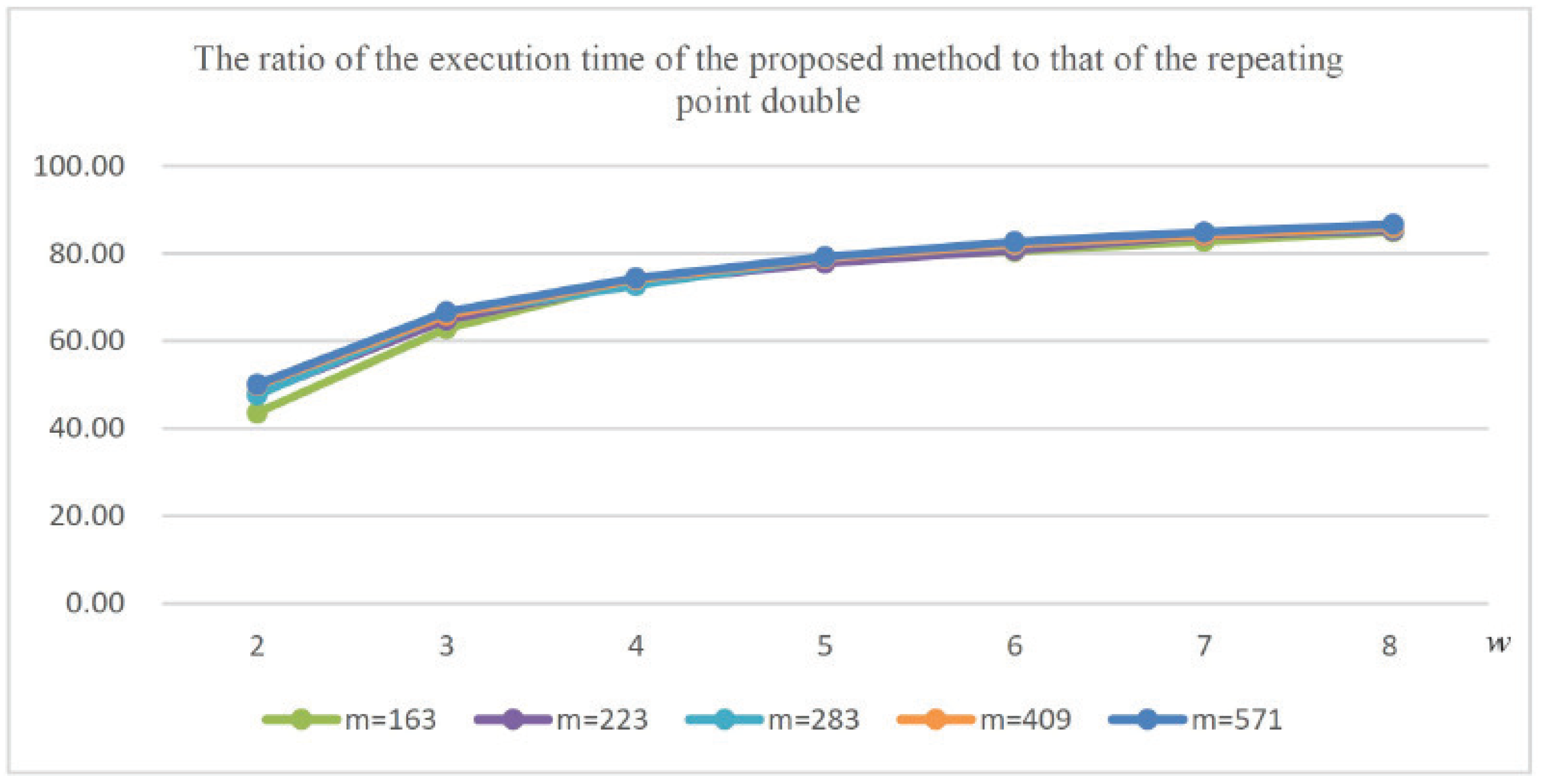
demonstrates the execution times of the Tradition algorithm and the PDNTimes algorithm involved in the ScalarMUL algorithm. In other words, in line 7 of the ScalarMUL algorithm, the computation of $2^{w}Q$ is compared using PDNTimes and Tradition. Let $t_{prev}$ and $t_{prop}$ denote the execution time of the previous method and the proposed method, respectively. Then, in the table, the decreasing ratio is given by

$$\begin{array}{c}\hfill {\displaystyle \frac{t_{prev}-t_{prop}}{t_{prev}}}\times 100\end{array}$$

(15)

When comparing the performance of Tradition with that of PDNTimes for different values of m, it is observed that while the reduction in inverse operations has led to a decrease in computation time, the increased number of multiplication and square operations in the formula results in a slowdown of the computation time reduction as n approaches 8. This trend is illustrated in Figure 1. This trend is attributed to the increase in word length, which leads to longer table construction times and a corresponding rise in memory consumption. Furthermore, as depicted in the figure, this behavior remains consistent across different values of m, indicating that the trade-off between reduced inversions and increased multiplication and square operations persists regardless of the specific parameters.

3.3. Reducing Square Operation Time

In the PDNTimes algorithm, there are many square operations in $t_i,v_i$, and $u_i$. To further reduce the computation time for scalar multiplication or repeating point doubling, precomputations for square operations are employed again. The method we propose below will enable the square operation to utilize three main operations: XOR, bit shifting, and table lookup. Recall that $A(x)={\sum }_{i=0}^{m-1}{a}_i{x}^i$ is a polynomial defined over $GF(2^m)$. Then, given an integer $w\ge 2$, let d and r be integers such that $m=w·d+r$ and $0\le r\le w-1$. Using Horner’s rule again (note that the m we are considering is odd),

$$\begin{array}{ccc}\hfill A^2(x)& \equiv & ((\cdots ((((\sum _{j=0}^{w-1}{a}_{m-w+j}{x}^{2j})x^{2w}+\sum _{j=0}^{w-1}{a}_{m-2w+j}{x}^{2j})x^{2w}\mathbf{mod}f(x)\hfill \\ & +& \sum _{j=0}^{w-1}{a}_{m-3w+j}{x}^{2j})x^{2w}+\sum _{j=0}^{w-1}{a}_{m-4w+j}{x}^{2j})x^{2w}\mathbf{mod}f(x)\hfill \\ & +& \cdots \hfill \\ & +& \sum _{j=0}^{w-1}{a}_{m-(d-1)w+j}{x}^{2j})x^{2w}+\sum _{j=0}^{w-1}{a}_{m-dw+j}{x}^{2j})x^{2r}\mathbf{mod}f(x)\hfill \\ & +& \sum _{j=0}^{r-1}{a}_j{x}^{2j}.\hfill \end{array}$$

(16)

In Equation (16), the computation of $A^2(x)$ involves sequentially evaluating the expression

$$\begin{array}{c}\hfill ((\sum _{j=0}^{w-1}{a}_{m-iw+j}{x}^{2j})x^{2w}+\sum _{j=0}^{w-1}{a}_{m-(i+1)w+j}{x}^{2j})x^{2w}\mathbf{mod}f(x)\end{array}$$

(17)

for increasing values of i. Similar to Equation (7) (respectively, Equation (8)), the expression ${\sum }_{j=0}^{w-1}{a}_{m-iw+j}{x}^{2j}$ (respectively, ${\sum }_{j=0}^{r-1}{a}_j{x}^{2j}$) represents a w-bit word, denoted as $(a_{w-1}^i,a_{w-2}^i,\cdots ,a_1^i,a_0^i)$ (respectively, $(a_{w-1}^{d+1},a_{w-2}^{d+1},\cdots ,a_1^{d+1},a_0^i)$). The result of computing ${\sum }_{j=0}^{w-1}{a}_{m-iw+j}{x}^{2j}$, for $1\le i\le d$, and ${\sum }_{j=0}^{r-1}{a}_j{x}^{2j}$ can be found in the entry $TE(a_{w-1},a_{w-2},\cdots ,a_0)$ in

Table 4. The precomputations for ${\sum }_{j=0}^{w-1}{a}_{m-iw+j}{x}^{2j}$.

$\mathit{TE}({\mathit{a}}_{\mathit{m}-\mathit{iw}+\mathit{w}-1},{\mathit{a}}_{\mathit{m}-\mathit{iw}+\mathit{w}-2},\cdots ,{\mathit{a}}_{\mathit{m}-\mathit{iw}+1},{\mathit{a}}_{\mathit{m}-\mathit{iw}})$	${\sum }_{\mathit{j}=0}^{\mathit{w}-1}{\mathit{a}}_{\mathit{m}-\mathit{iw}+\mathit{j}}{\mathit{x}}^{2\mathit{j}}$
$TE(0,0,\cdots ,0,0,0)$	0
$TE(0,0,\cdots ,0,0,1)$	1
$TE(0,0,\cdots ,0,1,0)$	$TE(0,0,\cdots ,0,1)<<2$
$TE(0,0,\cdots ,0,1,1)$	$TE(0,0,\cdots ,0,1)+TE(0,0,\cdots ,1,0)$
$TE(0,0,\cdots ,1,0,0)$	$TE(0,0,\cdots ,0,1,0)<<2$
$TE(0,0,\cdots ,1,0,1)$	$TE(0,0,\cdots ,0,1)+TE(0,0,\cdots ,1,0,0)$
⋮	⋮
$TE(1,1,\cdots ,1,1,1)$	$TE(1,0,\cdots ,0,0,0)+TE(0,1,\cdots ,1,1,1)$

provided that $a_{m-iw+j}=a_j$ for $0\le j\le w-1$. In the subsequent discussion, the notation “$•<<n$” will be used to denote shifting • to the left by n positions, with all the least significant bits set to zero, where n is a positive integer.

In Equation (17), since the maximum degree before applying the modulo operation with respect to $f(x)$ is less than m, the remainder obtained through traditional long division depends on the polynomial $f(x)+x^m$. The result of this modulo operation, denoted as $RD(r_{2w-1},r_{2w-2},\cdots ,r_0)$, is provided in

Table 5. The precomputations for (17). $f^{\prime }=f(x)+x^m$.

$\mathit{RD}({\mathit{r}}_{2\mathit{w}-1},{\mathit{r}}_{2\mathit{w}-2},\cdots ,{\mathit{r}}_0)$	Result
$RD(0,0,\cdots ,0,0,0)$	0
$RD(0,0,\cdots ,0,0,1)$	$f^{\prime }$
$RD(0,0,\cdots ,0,1,0)$	$f^{\prime }<<1$
$RD(0,0,\cdots ,0,1,1)$	$RD(0,0,\cdots ,0,0,1)+RD(0,0,\cdots ,0,1,0)$
$RD(0,0,\cdots ,1,0,0)$	$f^{\prime }<<2$
$RD(0,0,\cdots ,1,0,1)$	$RD(0,0,\cdots ,1,0,0)+RD(0,0,\cdots ,0,0,1)$
$RD(0,0,\cdots ,1,1,0)$	$RD(0,0,\cdots ,1,0,0)+RD(0,0,\cdots ,0,1,0)$
$RD(0,0,\cdots ,1,1,1)$	$RD(0,0,\cdots ,1,0,0)+RD(0,0,\cdots ,0,1,1)$
⋮	⋮
$RD(1,1,\cdots ,1,1,1)$	$RD(1,0,\cdots ,0,0,0)+RD(0,1,\cdots ,1,1,1)$

, which represents the remainder of (17). Table 5 comprehensively lists all possible outcomes for $r_{2w-1},r_{2w-2},\cdots ,r_0$.

Therefore, the square operation $A^2(x)\mathbf{mod}f(x)$ can be computed with the following Algorithm 4, SquareMod$(A,f,m,w)$.

Algorithm 4 SquareMod$(A,f,m,w)$
1.	Set  $C=(c_{2w-1},c_{2w-2},\cdots ,c_0)=(0,0,\cdots ,0),d=\lfloor {\displaystyle \frac{m}{w}}\rfloor ,r=m-w·d$
2.	Make table $TE$ and $RD$ such as Table 4 and Table 5, respectively
3.	For  $i=1$  to  $d-1$
4.	do
5.	$C\leftarrow C+TE(a_{m-iw+w-1},a_{m-iw+w-2},\cdots ,a_{m-iw+1},a_{m-iw})$
6.	$C\leftarrow C(x^{2w})+RD(c_{2w-1},c_{2w-2},\cdots ,c_0)$
7.	Enddo
8.	$C\leftarrow C+TE(a_{r+w-1},a_{r+w-2},\cdots ,a_{r+1},a_r)$
9.	$C\leftarrow C(x^{2r})+RD(c_{2w-1},c_{2w-2},\cdots ,c_0)$
10.	$C\leftarrow C+TE(0,0,\cdots ,0,a_{r-1},a_{r-2},\cdots ,a_1,a_0)$
11.	return C

In the SquareMod algorithm, for each iteration i, the result of the equation of Equation (17) is represented as $C=(c_{2w-1},c_{2w-2},\cdots ,c_1,c_0)$. In practical implementation, the term $x^{2w}$ in Equation (17) implies that each $c_j$ in C is shifted to the left by $2w$ positions, with all lower-order bits set to zero, where $0\le j\le 2w-1$. Let $m^{\prime }$ denote the maximum degree of the polynomial in Equation (17) before applying the modulo operation with $f(x)$, and let $f^{\prime }=f(x)+x^m$. As $A^2(x)$ is stored in an m-bit array in the code, there is a constraint on the shifting of C. Specifically, $m^{\prime }$ must be greater than the sum of $2w+1$ and the maximum degree of $f^{\prime }$. This ensures that the shifting operation does not exceed the bounds of the array and that the modulo operation can be correctly applied.

In the SquareMod algorithm, the computational time can be broken down as follows:

• Lines 5 and 6: Each iteration of the loop in these lines requires 2 XOR operations, 1 shift, and 2 table lookups.
• Lines 8–10: These lines consist of 3 XOR operations, 1 multiplication, and 3 table lookups.

Therefore, a total of $(2d+1)$ XORs, d shifts, and $(2d+1)$ table lookups are required. From the perspective of time complexity, this time is negligible compared with the time required for multiplication.

In the ScalarMUL and SquareMod algorithms, scalar multiplication corresponds to retrieving precomputed values stored in Table 1, Table 4, and Table 5. As a result, this approach significantly enhances computational efficiency by reducing the need for repeated calculations.

Lemma 3.

Given an integer w, the scalar multiplication of a point on $y^2+xy=x^3+A{x}^2+B$ over $GF(2^m)$ can be computed in $\lceil {\displaystyle \frac{m}{w}}\rceil$ iterations in the algorithms ScalarMUL and SquareMod.

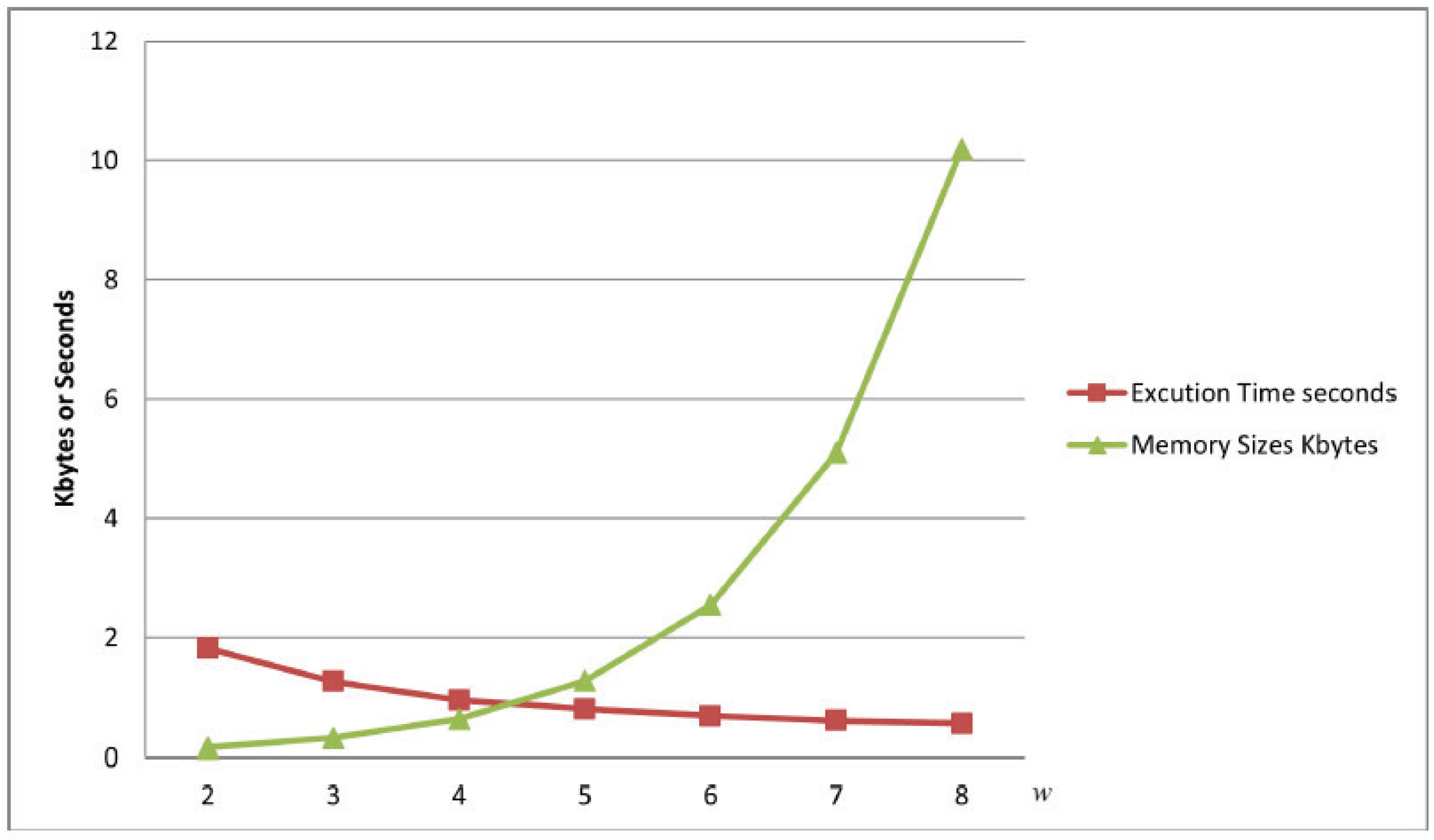
In Lemma 3, the $\lceil {\displaystyle \frac{m}{w}}\rceil$ iterations imply that a scalar multiplication of the form $2^{\lceil {\displaystyle \frac{m}{w}}\rceil }Q$ of a given point Q is performed on a given point Q. To evaluate the execution time of the SquareMod algorithm, a test code was implemented to execute the algorithm 100,000 times for each word length w with $2\le w\le 8$. Additionally, the memory size required for the lookup table in SquareMod was measured for each word length. For instance, in the case of $GF(2^{163})$,

Table 6. The execution time (seconds) and memory size ($2^w\times 163$ bits/8 bits) of the implementation of the SquareMod algorithm for $w=2,3,\dots ,8$ in computing $A{(x)}^2$ over $GF(2^{163})$.

w	Time	Memory Size
		$\mathit{RD}(•)$	$\mathit{TE}(•)$	Total
2	0.180	82	82	0.16
3	0.122	163	163	0.32
4	0.094	326	326	0.64
5	0.07	652	652	1.27
6	0.69	304	1304	2.55
7	0.060	2608	2608	5.09
8	0.054	5216	5216	10.19

summarizes the execution time and the corresponding memory size needed for the lookup table in SquareMod. Figure 2 provides a graphical representation of the data presented in Table 6. As evident from the table or figure, there is a trade-off between execution time and memory usage. While increasing the word length w can enhance computational efficiency, it also results in a significant increase in the memory size required and construction times for the lookup table. This highlights the need to carefully balance performance optimization with memory constraints when implementing the SquareMod algorithm. Finding the optimal word length will also determine the performance of scalar multiplication, meaning the efficiency of scalar multiplication is adjustable. Taking $GF(2^{163})$ as an example, in our program execution environment, the memory size required for each word length w is shown in

Table 7. The execution time and memory size ($2^w\times m$ bits/8 bits) of the ScalarMUL algorithm for $w=2,3,\dots ,8$ over $GF(2^m)$, where $m=163,233,283,409,571$. Note that the memory size does not include the $RD(•)$ and $TE(•)$ values listed in Table 6.

m	Time	w
	Size	2	3	4	5	6	7	8
163	seconds	1.18	0.83	0.71	0.70	0.83	1.22	2.07
	bytes	82	163	326	652	1304	2608	5216
233	seconds	3.36	2.32	1.89	1.81	2.08	2.79	4.46
	bytes	117	233	466	932	1864	3728	7456
283	seconds	6.44	4.46	3.63	3.40	3.62	4.85	7.47
	bytes	142	283	566	1132	2264	4528	9056
409	seconds	19.98	13.64	10.71	9.62	9.96	12.01	17.33
	bytes	205	409	818	1636	3272	6544	13,088
571	seconds	50.36	33.67	26.29	22.74	21.91	25.40	34.24
	bytes	286	571	1142	2284	4568	9136	18,272

. The execution time can be optimized by selecting an appropriate value of w based on the hardware and software specifications of the specific execution environment.

4. Inverse Algorithm Use ScalarMUL

ECC parameters over $GF(2^m)$ used in the ScalarMUL algorithm and the sliding window method [21] are provided in

Table A5. Recommended elliptic curve domain parameters over $GF(2^m)$.

$A=$ 0x1, $m=163,f(x)=x^{163}+x^7+x^6+x^3+1,f(x)+x^m=$ 0xc9
$x_0$	0x02FE13C0537BBC11ACAA07D793DE4E6D5E5C94EEE8
$y_0$	0x0289070FB05D38FF58321F2E800536D538CCDAA3D9
$A=$ 0x1, $m=233,f(x)=x^{233}+x^{74}+1,f(x)+x^m=$ 0x4000000000000000001
$x_0$	0x017232BA853A7E731AF129F22FF4149563A419C26BF50A4C9D6EEFAD6126
$y_0$	0x01DB537DECE819B7F70F555A67C427A8CD9BF18AEB9B56E0C11056FAE6A3
$A=$ 0x1, $m=283,f(x)=x^{283}+x^{12}+x^7+x^5+1,f(x)+x^m=$ 0x10a1
$x_0$	0x00FAC9DFCBAC8313BB2139F1BB755FEF65BC391F8B36F8F8EB7371FD558B
$y_0$	0x01006A08A41903350678E58528BEBF8A0BEFF867A7CA36716F7E01F8105
$A=$ 0x1, $m=409,f(x)=x^{409}+x^{87}+1,f(x)+x^m=$ 0x8000000000000000000001
$x_0$	0x0060F05F658F49C1AD3AB1890F7184210EFD0987E307C84C27ACCFB8F9F67C
	C2C460189EB5AAAA62EE222EB1B35540CFE9023746
$y_0$	0x01E369050B7C4E42ACBA1DACBF04299C3460782F918EA427E6325165E9EA10E
	3DA5F6C42E9C55215AA9CA27A5863EC48D8E0286B
$A=$ 0x1, $m=571,f(x)=x^{571}+x^{10}+x^5+x^2+1,f(x)+x^m=$ 0x425
$x_0$	0x026EB7A859923FBC82189631F8103FE4AC9CA2970012D5D46024804801841CA4
	4370958493B205E647DA304DB4CEB08CBBD1BA39494776FB988B47174DCA88C
	7E2945283A01C8972
$y_0$	0x0349DC807F4FBF374F4AEADE3BCA95314DD58CEC9F307A54FFC61EFC006D
	8A2C9D4979C0AC44AEA74FBEBBB9F772AEDCB620B01A7BA7AF1B320430C85
	91984F601CD4C143EF1C7A3

of Appendix A. The execution times for each word length, both with and without the formulas utilized in the ScalarMUL algorithm, as well as for each window size in the sliding window method [21], are presented in

Table 8. The execution times (seconds) for the ScalarMUL algorithm (both the PDNTimes and SquareMod algorithms are utilized) and sliding window method [21] over $GF(2^m)$.

m	Methods	Window Size or Word Length, w
		2	3	4	5	6	7	8
163	Sliding window	1.72	1.51	1.42	1.43	1.48	1.67	2.08
	ScalarMUL without formulas	1.66	1.50	1.46	1.50	1.73	2.13	2.98
	ScalarMUL with formulas	1.18	0.83	0.71	0.70	0.83	1.22	2.07
233	Sliding window	5.08	4.51	4.21	4.14	4.25	4.58	5.44
	ScalarMUL without formulas	4.96	4.44	4.31	4.32	4.63	5.46	7.18
	ScalarMUL with formulas	3.36	2.32	1.89	1.81	2.08	2.79	4.46
283	Sliding window	9.60	8.56	8.08	7.98	8.09	8.59	9.89
	ScalarMUL without formulas	9.48	8.49	8.10	8.24	8.71	9.88	12.6
	ScalarMUL with formulas	6.44	4.46	3.63	3.40	3.62	4.85	7.47
409	Sliding window	29.97	26.57	24.93	24.30	24.14	25.24	27.96
	ScalarMUL without formulas	29.54	26.31	24.98	24.80	25.71	28.44	34.29
	ScalarMUL with formulas	19.98	13.64	10.71	9.62	9.96	12.01	17.33
571	Sliding window	74.58	66.62	63.20	61.38	60.52	61.29	66.18
	ScalarMUL without formulas	74.17	67.25	62.87	61.56	61.61	65.59	76.50
	ScalarMUL with formulas	50.36	33.67	26.29	22.74	21.91	25.40	34.24

. Note that the scalar k used in the algorithm ScalarMUL and the sliding window are the extension degree m of $GF(2^m)$. Additionally,

Table 9. For $m=163,233,283,409,571$, on $w=2,3,\dots ,8$ over $GF(2^m)$, the decreasing ratio for the ScalarMUL algorithm with formulas for the sliding window method [21] and the sliding window method with formulas to the sliding window method.

m	Algorithm	w
		2	3	4	5	6	7	8
163	ScalarMUL	31	45	50	51	44	27	0.5
	sliding window	33	47	55	58	57	52	43
233	ScalarMUL	34	49	55	56	51	39	18
	sliding window	34	49	56	60	61	57	49
283	ScalarMUL	33	48	55	57	55	44	24
	sliding window	34	48	58	62	64	61	54
409	ScalarMUL	33	49	57	60	59	52	38
	sliding window	33	49	58	64	65	65	59
571	ScalarMUL	32	49	58	63	64	59	48
	sliding window	32	50	58	64	67	68	64

illustrates the decreasing ratio, which compares the execution time of the proposed method with that of the sliding window method  [21], highlighting the efficiency improvements achieved by the proposed approach. The decreasing trend in execution time is illustrated in Figure 3. The proposed formulas are specifically tailored for scenarios that involve repeating point-doubling operations, enabling a significant reduction in the number of inverse operations required. The application of our proposed method to the sliding window technique simply requires replacing the formulas we derived for repeating point doubling in Algorithm 2 in [21] with our proposed formulas. Furthermore, these formulas can be seamlessly integrated into the sliding window method to further improve its computational efficiency, as demonstrated by the results presented in Table 9. From Table 9, we observe that the sliding window method with formulas exhibits better efficiency. This is because the sliding window method utilizes a window based on the positions of the bit 1s in the binary representation of k for repeated point doubling. In contrast, our method uses a fixed word length, which requires more precomputation. However, this also demonstrates the value of our derived formulas. This integration highlights the versatility and effectiveness of the proposed approach in optimizing elliptic curve operations.

Over $GF(2^m)$, given a point Q, word length w, and setting $n=m$, Figure 4 illustrates the advantages of the PDNTimes algorithm in reducing the number of inverse operations required. In line 7 of the ScalarMUL algorithm, the operation $Q\leftarrow 2^{w}Q$ requires computing $2^{w}Q$, which involves performing w consecutive point doublings on the point Q. We compare the performances based on the number of multiplication operations required. In finite fields, the performance is largely determined via the inverse operations, as they require multiple multiplication operations to compute. The exact number of multiplications depends on the algorithm used. For example, if the Extended Euclidean Algorithm is used, an inverse operation generally takes about $2m$ to $3m$ multiplications, depending on the implementation’s optimization. The exact number of multiplications required for an inverse operation using Fermat’s Little Theorem is $m-2$. In line 13 of the PDNTimes algorithm, we utilize Fermat’s Little Theorem to compute the inverse $t_n^{\prime }$. For the PDNTimes algorithm, $(m-2)+6w$ multiplication operations are required. If we replace the computation of $Q\leftarrow 2^{w}Q$ in line 7 of PDNTimes with Equation (2) (in line 4 of Tradition) to compute $2^{w}Q$, we will require $w(m-2)+2w$ multiplication operations.

In the affine coordinate system, both point addition and point doubling require one inverse to compute the slope $\lambda$. Additionally, each operation involves five multiplications, as follows:

• Two multiplications for calculating $\lambda$;
• Two multiplications for determining the new x-coordinate;
• One multiplication for determining the new y-coordinate.

Although our algorithm demonstrates reduced time complexity compared with the sliding window method, as shown in

Table 10. Summary of the number of operations required for scalar multiplication over $GF(2^m)$ in the affine coordinate system.

Algorithm	Multiplications	Inverse Operations
Double and Add [22]	$7.5m$	${\displaystyle \frac{3m}{2}}$
Sliding Window	$5m+{\displaystyle \frac{5m}{w+1}}$	$m+{\displaystyle \frac{m}{w+1}}$
Montgomery Ladder [23]	$10m$	$2m$
The proposed methods	$m-2+6w$	1

, its practical execution requires the construction of a larger lookup table. As a result, while our approach still outperforms the sliding window method in terms of efficiency, the performance gap is not as significant as indicated in Table 10.

5. Conclusions

In this work, we focused on significantly reducing the computation time of scalar multiplication, which can be easily implemented in software, by further expanding the application of Horner’s rule and optimizing the square operations, specifically, through the introduction of several formulas for the inverse operations involved in repeating point doubling.

In elliptic curve cryptography and other cryptographic protocols, scalar multiplication is a critical operation that can be computationally expensive, primarily due to the repeated use of inverses and point doubling, which are key to optimizing efficiency.

The introduced formulas can help to minimize the number of inverse operations needed, thereby streamlining the computational process. Computation using the introduced formulas for ${\lambda }_n$ and $x_n$ requires more multiplication, square, and addition operations. We also developed the ScalarMod algorithm to reduce the computation time for square operations.

Figure 1 demonstrates that if the ScalarMul algorithm does not optimize for square operations, the overall reduction in computation time begins to plateau when the word length w reaches 8. This highlights the importance of optimizing square operations to achieve consistent performance improvements. On the other hand, Figure 2 illustrates that while the Square algorithm optimizes square operations, a trade-off must be made between execution time and the required memory size. These two phenomena represent key challenges that we aim to overcome and improve upon in future work.

From a theoretical perspective, analyzing the trade-off between execution time and memory usage is an intriguing research topic and a promising direction for future exploration. Understanding this balance could lead to more efficient algorithms that are both fast and resource efficient, making them suitable for a wider range of applications, including resource-constrained environments such as embedded systems and IoT devices.

On the other hand, an important consideration lies in the potential trade-offs between security and implementation complexity. While the primary focus of our work was to reduce the number of inverse operations in scalar multiplication—a critical bottleneck in ECC—any optimization technique must be carefully assessed for its impact on both security and practical implementation.

• Security Considerations
  Our proposed method is based on well-established mathematical principles and does not introduce new assumptions or structures that could weaken the cryptographic security of the system. The repeating point-doubling formulas and grouping technique are derived directly from the affine coordinate system, ensuring that the underlying security properties of the elliptic curve are preserved. However, we recognize that side-channel attacks (e.g., timing or power analysis) could still pose a risk, as with any cryptographic implementation. While our current work does not explicitly address side-channel resistance, we plan to investigate this aspect in future research, potentially integrating countermeasures such as constant-time execution or masking techniques.
• Implementation Complexity
  The proposed method is designed to be simple and consistent in execution, making it suitable for both software and hardware implementations. The grouping technique and modified Horner’s rule introduce minimal overhead in terms of precomputation and memory usage, as the bit-words and repeated point-doubling results can be efficiently stored and reused. Our approach achieves faster scalar multiplication with a comparable level of implementation complexity in comparison with traditional methods like the sliding window algorithm. That said, we acknowledge that further evaluation is needed to assess its performance in highly resource-constrained environments, such as IoT devices or embedded systems.
• Future Work
  While our initial results demonstrate significant improvements in computational efficiency, we agree that a more comprehensive evaluation of security and implementation complexity is essential. Future work will involve the following:
  • A thorough security analysis, including resistance to side-channel attacks;
  • Evaluation of the performance of methods in a wider range of hardware and software environments; particularly in resource-constrained settings.
  • Comparison of the proposed method with other state-of-the-art techniques to identify potential trade-offs and optimize its practical applicability.

Finally, the formulas we derived are completely independent of B in the elliptic curve equation $E(x,y):y^2+xy=x^3+A{x}^2+B$. This independence simplifies the application of our formulas across different elliptic curves. However, we are also curious whether it is possible to derive formulas that are independent of the parameter A in the equation. Exploring this possibility could lead to even more generalized and versatile results, potentially opening new avenues for optimization in elliptic curve cryptography. Such advancements could further enhance the efficiency and applicability of cryptographic protocols in real-world scenarios.