Abstract
A system of inhomogeneous second-order difference equations with linear parts given by noncommutative matrix coefficients are considered. The closed form of its solution is derived by means of a newly defined delayed matrix sine/cosine using the transform and determining function. This representation helps with analyzing iterative learning control by applying appropriate updating laws and ensuring sufficient conditions for achieving asymptotic convergence in tracking.
MSC:
39A06; 93C55; 93C40
1. Introduction
Second-order delayed difference equations are crucial in real-world applications because they model dynamic systems where the future state depends not only on the current and past states but also on delayed interactions. These equations arise in various domains, including population dynamics, where they are used to model species growth with delayed responses due to gestation or maturation periods; economic systems, being applied in financial markets and supply chain modeling where past fluctuations influence current trends; engineering and control systems, where they are found in signal processing, vibration analysis, and control systems where delays affect stability and performance; epidemiology, being used to model the spread of diseases where incubation periods and immunity delays play a role.
The proposed method improves upon existing techniques in several ways:
Enhanced stability analysis—it provides new stability criteria that better capture the effects of delays, reducing uncertainties in predictions; Higher computational efficiency—the method optimizes numerical computations, allowing for faster simulations and real-time applications; Broader applicability—it extends to more complex and nonlinear systems, making it useful for modeling real-world phenomena with varying delay structures; Improved accuracy—by refining approximation methods or incorporating machine learning techniques, the approach yields more precise solutions. These advancements contribute to more reliable modeling, better decision making, and improved system performance across multiple disciplines.
The proposed method may face significant challenges when dealing with singular matrices or nonpermutable coefficients due to the following reasons:
Limitations exist in handling singular matrices. Singular matrices lack an inverse, which can hinder solving linear systems directly. Many numerical techniques, including those used for stability analysis and iterative solutions, rely on matrix inversion or decomposition, which fails in the singular case. This limitation restricts the method’s applicability to systems where the coefficient matrices are nonsingular or can be regularized (e.g., by perturbation methods or pseudo-inverses). There are limitations with nonpermutable coefficients. If the system involves coefficients that do not commute under multiplication (e.g., in noncommutative algebra or certain coupled systems), traditional solution techniques may not directly apply. Many iterative or closed-form solutions assume a structure that allows for the reordering of terms, which may not hold in these cases. This constraint affects applications in quantum mechanics, advanced control systems, and coupled network dynamics where nonpermutable interactions are essential. The method remains effective for a broad class of second-order delayed difference equations with well-conditioned coefficient structures. For singular matrices, alternative techniques like regularization, generalized inverses, or alternative formulations may be necessary. For nonpermutable coefficients, more advanced algebraic methods or computational techniques may need to be incorporated, potentially requiring significant modifications to the proposed approach. If these extensions are not currently feasible, it should be explicitly stated that the method is best suited for nonsingular, permutable coefficient systems, and potential workarounds or future research directions should be proposed.
The proposed method can be highly beneficial in ILC systems, where tasks are performed repeatedly, and performance is improved over iterations by learning from past errors. Below are concrete examples where the method could be applied:
- Trajectory tracking in robotics: in robotic arms used for precision tasks (e.g., surgical robots, automated welding arms), trajectory tracking is critical.
- ILC is often used to refine movement paths over successive iterations, compensating for dynamic disturbances and model inaccuracies.
- The second-order delayed difference equation framework models the system’s response more accurately, accounting for actuator delays and sensor latencies.
- The improved stability analysis ensures better convergence of the learning process, reducing oscillations or divergence issues in robot movements.
- Compared to traditional ILC methods, this approach can handle systems with more complex dynamics and variable delays, leading to faster convergence and smoother trajectory tracking.
By leveraging the proposed method, industries relying on precision control, automation, and iterative improvements can achieve higher accuracy, efficiency, and adaptability, making it a significant advancement in ILC applications.
In what follows, we use the following notations:
- is a zero matrix, and I is an identity matrix;
- for , ;
- is the space of matrices;
- An empty sum , and an empty product for integers , where is a given function that does not have to be defined for each in this case;
- is the forward difference operator;
Iterative learning control (ILC) is a control strategy used for systems that perform the same task repeatedly. It improves performance over iterations by learning from previous executions. The idea is to adjust the control input based on errors from past trials, refining it until the desired performance is achieved.
Key Concepts of ILC
- Repetitive tasks: ILC is useful in systems where the same task is performed multiple times, such as robotic arms, industrial automation, and medical rehabilitation devices.
- Error correction: the controller updates the input signal for the next iteration based on the difference between the desired and actual output from the previous iteration.
- Feedforward control: unlike traditional feedback control, ILC predicts and compensates for errors before they occur in future iterations.
- Convergence: a well-designed ILC algorithm ensures that the system output approaches the desired output over iterations.
General ILC Algorithm
The control input for iteration is updated as
where is the control input at iteration k, is the error at iteration k (the difference between the desired and actual output), and L is the learning filter or gain.
Applications of ILC
- Robotics: improving precision in repetitive tasks.
- Industrial automation: enhancing accuracy in machining and assembly lines.
- Medical applications: assisting in rehabilitation by improving repetitive movements.
- Motion control: used in servo systems to improve trajectory tracking.
ILC is a powerful control strategy designed for dynamic systems that operate repetitively over a finite time interval. It has been successfully implemented in various practical applications, including robotics, chemical batch processes, and hard disk drive systems, as highlighted in References [1,2,3,4] and the works cited therein.
In recent years, considerable attention has been given to the iterative learning control and robust control of discrete systems by many researchers. Notably, Li et al. [5] investigated ILC for linear continuous systems with time delays using two-dimensional system theory. Similarly, Wan [6] studied ILC for two-dimensional discrete systems under a general model. Extensive research on ILC for discrete systems has often been carried out by analyzing a constructed Roesser model, as demonstrated in References [5,6,7,8]. To the best of our knowledge, the application of the Roesser model to ILC for discrete systems was initially explored in Reference [2].
Approximately two decades ago, Diblik and Khusainov [9,10] introduced explicit representations for solutions to discrete linear systems with a single pure delay using delayed discrete exponential matrices. Later, Khusainov et al. [11] extended this approach to derive analytical solutions for oscillatory second-order systems with pure delays by introducing delayed discrete sine and cosine matrices. These pioneering contributions spurred significant advancements in the analytical solutions of retarded integer and fractional differential equations, as well as delayed discrete systems, as seen in References [12,13,14,15]. Building on these results, Diblik and Morçivkova [16,17] extended the analysis to discrete linear systems with two pure delays, while Pospişil [18] applied the transform to address multi-delayed systems with linear components represented by permutable matrix coefficients. In 2018, Mahmudov [19] provided explicit solutions for discrete linear delayed systems with nonconstant coefficients and nonpermutable matrices, including first-order differences. Mahmudov [20] later generalized these findings, removing the singularity condition on the non-delayed coefficient matrix and deriving explicit solutions using the transform. Furthermore, Diblik and Mencakova [12] presented closed-form solutions for purely delayed discrete linear systems with second-order differences, while Elshenhab and Wang [21] recently addressed explicit representations for second-order difference systems with multiple pure delays and noncommutative coefficient matrices.
These studies have yielded numerous insights into the qualitative theory of discrete delay systems, encompassing stability analysis, optimal control theory, and iterative learning control, as highlighted in References [22,23,24,25,26,27].
Although significant progress has been made in studying linear discrete systems and linear delayed discrete systems, research on iterative learning control for delayed linear discrete systems with higher-order differences remains limited. Notable examples include References [6,7], with only a few works addressing delayed linear discrete systems with higher-order differences through the construction of delayed discrete matrix functions.
Therefore, motivated by [12,19,21], we consider an explicit representation of solutions of the following discrete second-order systems with a single delay:
where m is a delay, , is a solution, and is a function.
Let be a function. We attach to (1) the following initial conditions:
It is well known that the initial value problem (1) and (2) has a unique solution in .
More precisely, we study the iterative learning control problem for delayed linear discrete systems with a second-order difference as follows:
where k denotes the kth iteration, T is a given fixed positive integer, denotes the state, denotes the dominant input, and denotes the output. , are constant matrices.
Here is a summary of the key contributions:
- This work introduces new delayed discrete matrix functions, which are regarded as extensions of the sine and cosine functions.
- New representation of solutions: This work proposes a new representation for the solutions for the second-order delay difference equations with noncommutative matrices. This representation is likely used in various aspects of this paper, including deriving the prior estimation of the state. This representation is new even for the second-order difference equations with commutative matrices.
- Application to convergence laws and iterative learning control: the new solution representations are applied to derive convergence laws for ILC systems, providing insights into the convergence behavior of the system via the proposed iterative learning control updating laws.
- Extension of ILC problems: this work extends iterative learning control to address problems involving second-order delay difference equations with noncommutative matrices, potentially presenting new methods or solutions for ILC in these contexts.
2. Delayed Discrete Matrix Sine/Cosine
One of the tools in this study is the transform, defined as
transform is considered component-wisely, i.e., the transform of a vector-valued function is a vector of -transformed coordinates.
Definition 1.
We say that the function is exponentially bounded if there exists such that
Lemma 1.
The transform of exponentially bounded function exists for all sufficiently large z.
The next lemma provides some features of the transform.
Lemma 2.
Assume that are exponentially bounded functions. Then, for sufficiently large , we have
- 1.
- 2.
- for where δ is the Kroneker delta,
- 3.
- . Here, the convolution operation ∗ is defined by
- 4.
- for ; here, σ is the step function, defined as
- 5.
- , .
- 6.
- ,
We introduce the determining matrix equation for
where I is an identity matrix; is a zero matrix.
Remark 1.
- 1.
- Simple calculations show that
- 2.
- If A and B are commutative, that is, , we have
- 3.
- If , then
Definition 2.
The delayed discrete matrix is defined as
Here,
- Θ represents the zero matrix.
- I is the identity matrix.
- denotes the binomial coefficient, defined as , with if or .
Definition 3
([12]). The delayed discrete matrix is defined as
Definition 4
([12]). The delayed discrete matrix sine/cosine is defined as follows:
Remark 2.
If , then
Lemma 3
(Binomial formula for noncommutative matrices). Let be two noncommutative matrices. Then, for any , we have
Proof.
Lemma 4
(Gronwall inequality [28]). Let
Then,
Lemma 5.
For any , we have the following identities:
Proof.
The first two identities follow from Lemma 3. We start with the identity
For sufficiently large , such that
we derive
Next, we use the formulas
and
Now, consider the inverse transform of the original series:
Using similar steps for , we find
For the third transform, we have
□
Definition 5.
The delayed discrete matrix sine/cosine is defined as follows:
Lemma 6.
For all one has
where
Proof.
We only have the first inequality:
□
Lemma 7.
Proof.
Summing the above equality from 0 to , we obtain
equivalently
Taking the norm and applying the triangle inequality, we have
In this stage, without losing generality, it is assumed that Then,
Thus,
From the Gronwall inequality,
Therefore, one can easily see that there exists constants such that
□
3. Explicit Solutions
Below, we state and prove the main theorem of this paper. The main instrument used is the transform. We give a closed analytical form of the solution of problem (1), (2) in terms of the delayed discrete matrix sine/cosine.
Theorem 1.
Proof.
We recall that Lemma 7 says that the transform of the solution of (1) exists. Therefore, one can apply the transform to both sides of the delayed system (1) to obtain
This implies
In order to obtain an explicit form of we take the inverse transform to have
where
Using Lemma 5, we obtain the desired representation (7). □
Lemma 8.
and satisfy the following equations:
Proof.
The condition is an exponentially bounded can be eliminated through direct verification, that is why the proof of the following theorem is not included.
4. Convergence Results
Lemma 9
([29] Chapter 5.6). For a matrix and , there exists a matrix norm such that
where denotes the spectral radius of matrix A.
The proof provided is a detailed and rigorous mathematical argument demonstrating the convergence of the error sequence in the norm under the given conditions. Below are some clarifications and highlights for better understanding:
- Key assumption: the inequalityensures that the spectral radius of matrix is less than 1, which is a critical condition for the contraction and convergence of the error sequence.
- Iterative relation: the proof builds upon the iterative equation that expresses the evolution of error as a combination of the previous error and additional terms influenced by C, F, and .
- Norm bound: by bounding the -norm of the error, the proof systematically shows that the error decreases geometrically is controlled by choosing an appropriate within the specified range.
- Choice of the selection of is crucial.
- Convergence: the resultwith implies that the sequence converges to 0 as .
Let be a desired reference trajectory, and
Here, and represent the kth iteration error.
Introduce and . We construct the following P-type learning law:
When , we set
where and are learning gain parameter matrices determined in (21) and (27), respectively. Thus, from (3),
Taking account of (3) together with (15) and (17), separately, we are ready to give the convergence analysis for in the following two theorems.
Theorem 3.
Proof.
For (3) with , according to (15), we can obtain the relation between the kth error and the th error:
According to (17), we have
Taking norm on for (22) and from Lemma 9, we have
where is an arbitrary positive number.
When , obviously, , , and become d-dimensional zero vectors. According to (21) and (23), it is easy to obtain
When , multiplying both sides of (23) by and then taking the norm, we have
Now, we estimate the value of . According to (6), (17), and (19), we have
Taking the supremum norm for both sides of (25), we obtain
Now linking (24) and (26), we have
where
By (21), one derives
when
Finally, we obtain
which implies
□
Proof.
For (3) with and , we can obtain the relation between the kth error and the th error via (16):
Substituting (20) into (28), we obtain
Due to (15) and (18), we have
Taking norm for (29) and from Lemma 9, we have
for . From (27), it is easy to obtain
When , we have
Then, by taking the norm, we obtain
where and
We choose from the set
and, according to (30), we have
which means that
Thus, the proof is completed. □
5. Applicaitons
5.1. Example 1
We consider the discrete-time system:
where
The goal is to track a desired trajectory by iteratively updating the control input. We apply a P-type ILC update:
where is the tracking error, and L is the learning gain matrix:
The error propagation follows:
Compute
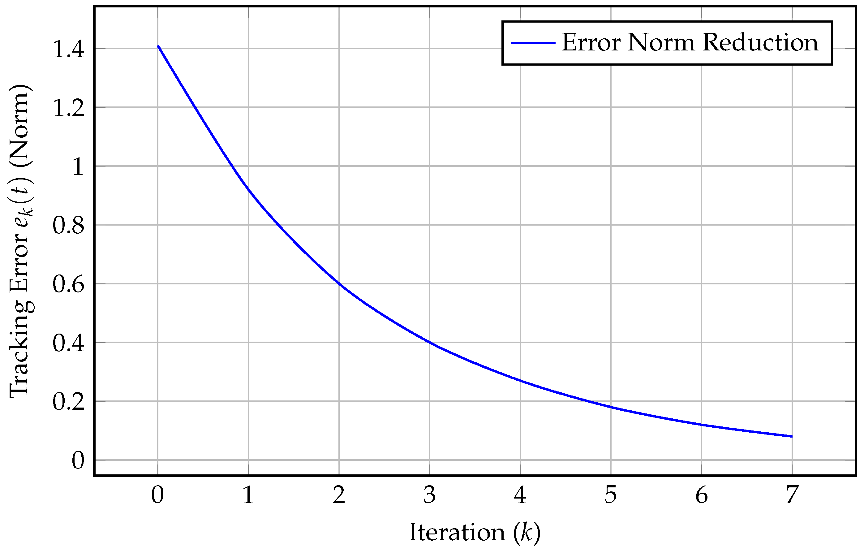
Since , the error decreases over iterations, ensuring convergence.
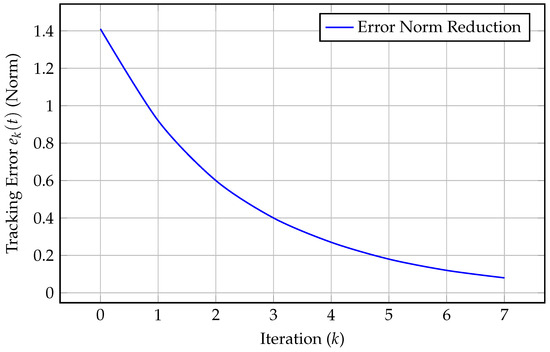
Figure 1.
Tracking error norm reduction over iterations.
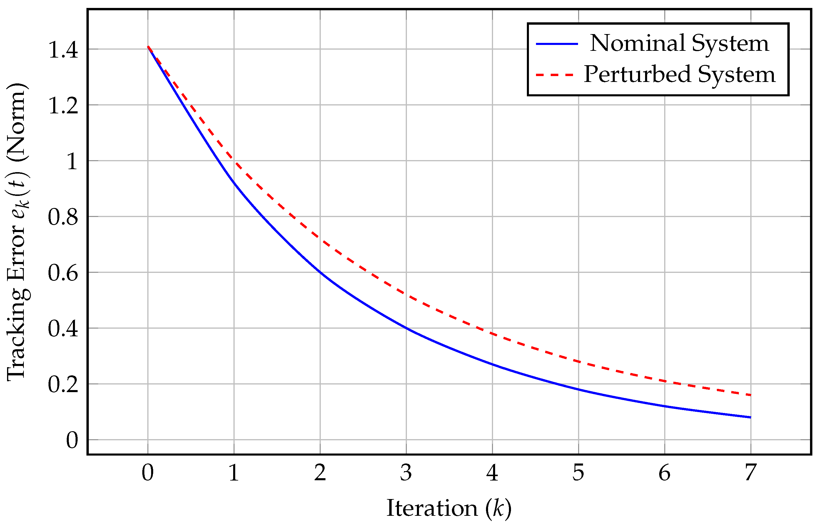
5.2. Perturbed System Model
We introduce small perturbations to matrices A and B:
Assume that
Thus, the perturbed system is
With this uncertainty, the new error propagation becomes
Compute :
The perturbed system still converges but more slowly due to increased error propagation (Figure 2):

Figure 2.
Tracking error norm over iterations for nominal and perturbed systems.
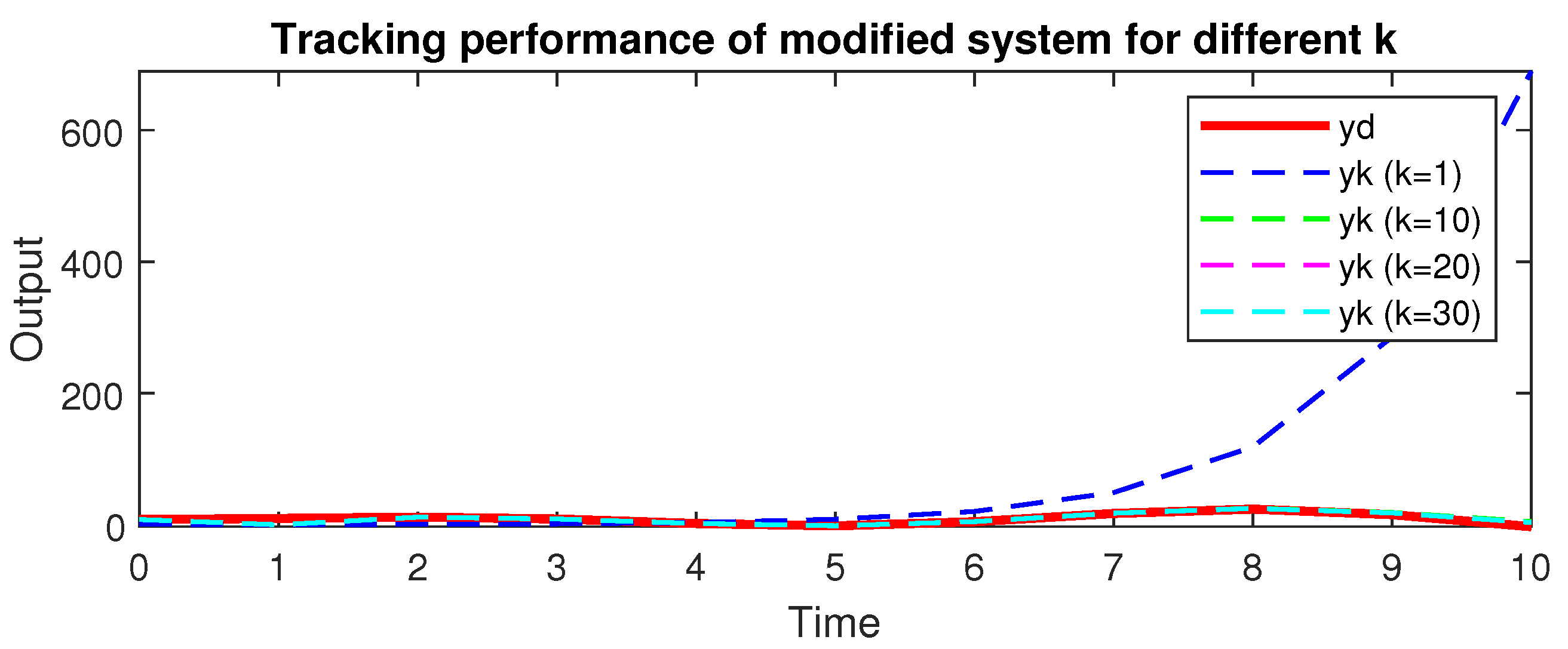
5.3. Example 2
We consider a discrete-time second-order linear system in two dimensions:
The control input is updated iteratively as
where the tracking error is given by
Since , the error decreases over iterations, ensuring convergence.
Figure 3 illustrates the system output compared to the desired trajectory over different iterations. The system aims to align with the desired trajectory as the iterations increase.
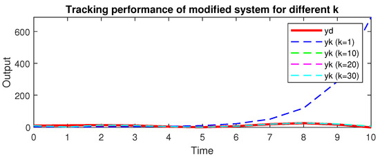
Figure 3.
System output trajectory over multiple iterations.
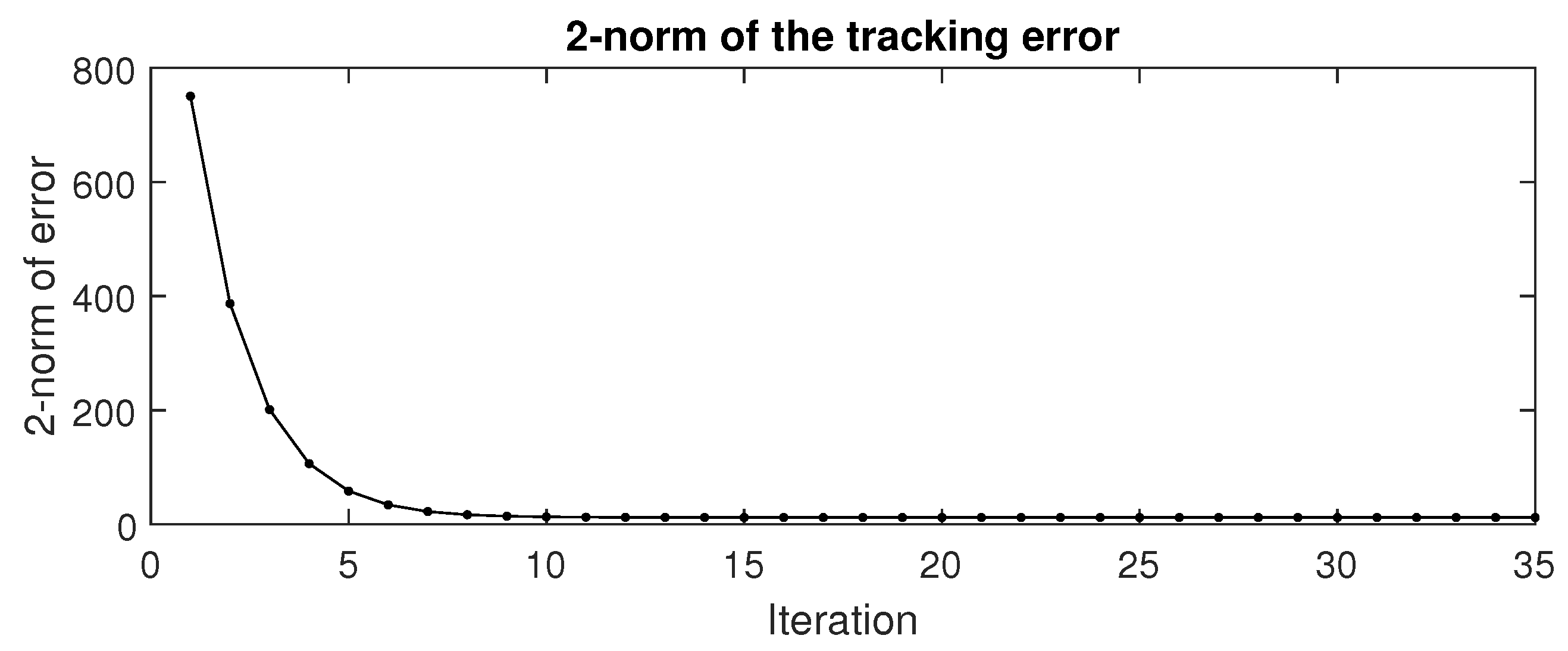
Figure 4 shows the error norm decreasing over time, demonstrating the convergence of the ILC process.

Figure 4.
Error norm over time steps.
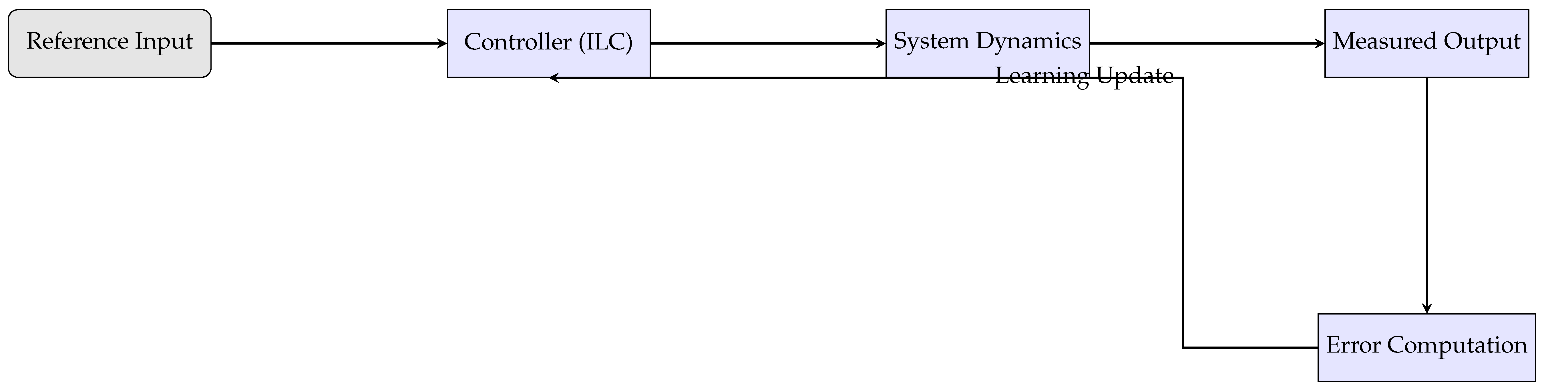
The ILC approach effectively refines the control input to improve trajectory tracking. The figures demonstrate the system’s convergence as errors reduce over iterations (Figure 5).
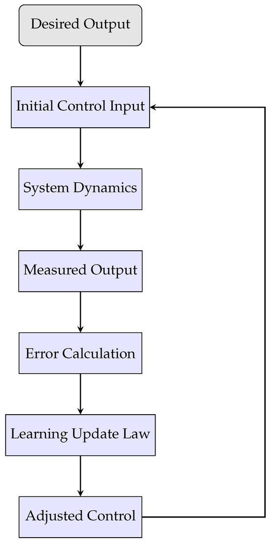
Figure 5.
Flowchart of an iterative learning control.
Block Diagram of an ILC System
6. Conclusions
A system of inhomogeneous second-order difference equations with linear parts given by noncommutative matrix coefficients was considered. The closed-form solution was derived using newly defined delayed matrix sine/cosine functions via the Z transform and determining function. This representation helped analyze iterative learning control by applying appropriate updating laws and ensuring sufficient conditions for achieving asymptotic convergence in tracking.
Future work may focus on controllability, stability, existence and uniqueness problems of multiple delayed discrete semilinear/linear systems.
Author Contributions
Conceptualization, N.I.M. and M.A. (Muath Awadalla); methodology, N.I.M.; validation, N.I.M., M.A. (Muath Awadalla) and M.A. (Meraa Arab); investigation, N.I.M., M.A. (Muath Awadalla) and M.A. (Meraa Arab); writing—original draft preparation, N.I.M. and M.A. (Muath Awadalla); writing—review and editing, N.I.M., M.A. (Muath Awadalla) and M.A. (Meraa Arab). All authors have read and agreed to the published version of this manuscript.
Funding
This work was supported by the Deanship of Scientific Research, Vice Presidency for Graduate Studies and Scientific Research, King Faisal University, Saudi Arabia [Grant No. KFU250955].
Data Availability Statement
Data are contained within this article.
Acknowledgments
This work was supported by the Deanship of Scientific Research, Vice Presidency for Graduate Studies and Scientific Research, King Faisal University, Saudi Arabia [Grant No. KFU250955].
Conflicts of Interest
The authors declare no conflicts of interest.
References
- Arimoto, S.; Kawamura, S.; Miyazaki, F. Bettering operation of robots by learning. J. Robot. Syst. 1984, 1, 123–140. [Google Scholar] [CrossRef]
- Sun, M.X.; Huang, B.J. Iterative Learning Control; National Defense Industry Press: Beijing, China, 1999. [Google Scholar]
- Bristow, D.A.; Tharayil, M.; Alleyne, A.G. A survey of iterative learning control. IEEE Control Syst. Mag. 2006, 26, 96–114. [Google Scholar]
- Ahn, H.S.; Chen, Y.Q.; Moore, K.L. Iterative learning control: Brief survey and categorization. IEEE Trans. Syst. Man Cybern. C Appl. Rev. 2007, 37, 1099–1121. [Google Scholar] [CrossRef]
- Li, X.D.; Chow, T.W.S.; Ho, J.K.L. 2-D system theory based iterative learning control for linear continuous systems with time delays. IEEE Trans Circuits Syst. I Regul. Pap. 2005, 52, 1421–1430. [Google Scholar]
- Wan, K. Iterative learning control of two-dimensional discrete systems in general model. Nonlinear Dyn. 2021, 104, 1315–1327. [Google Scholar] [CrossRef]
- Zhu, Q.; Xu, J.; Huang, D.; Hu, G. Iterative learning control design for linear discrete-time systems with multiple high-order internal models. Automatica 2015, 62, 65–76. [Google Scholar] [CrossRef]
- Wei, Y.S.; Li, X.D. Iterative learning control for linear discrete-time systems with high relative degree under initial state vibration. IET Control Theory Appl. 2016, 10, 1115–1126. [Google Scholar] [CrossRef]
- Diblík, J.; Khusainov, D.Y. Representation of solutions of discrete delayed system y(k + 1) = Ay(k) + By(k − m) + f(k) with commutative matrices. J. Math. Anal. Appl. 2006, 318, 63–76. [Google Scholar] [CrossRef]
- Diblík, J.; Khusainov, D.Y. Representation of solutions of linear discrete systems with constant coefficients and pure delay. Adv. Differ. Equ. 2006, 2006, 1–13. [Google Scholar] [CrossRef]
- Khusainov, D.Y.; Diblík, J.; Růžičková, M.; Lukáčová, J. Representation of a solution of the Cauchy problem for an oscillating system with pure delay. Nonlinear Oscil. 2008, 11, 276–285. [Google Scholar] [CrossRef]
- Diblík, J.; Mencáková, K. Representation of solutions to delayed linear discrete systems with constant coefficients and with second-order differences. Appl. Math. Lett. 2020, 105, 106309. [Google Scholar] [CrossRef]
- Elshenhab, A.M.; Wang, X.T. Representation of solutions for linear fractional systems with pure delay and multiple delays. Math. Methods Appl. Sci. 2021, 44, 12835–12860. [Google Scholar] [CrossRef]
- Elshenhab, A.M.; Wang, X.T. Representation of solutions of linear differential systems with pure delay and multiple delays with linear parts given by non-permutable matrices. Appl. Math. Comput. 2021, 410, 126443. [Google Scholar] [CrossRef]
- Pospíšil, M. Representation of solutions of systems of linear differential equations with multiple delays and nonpermutable variable coefficients. Math. Model. Anal. 2020, 25, 303–322. [Google Scholar] [CrossRef]
- Diblík, J.; Morávková, B. Discrete matriy delayed eyponential for two delays and its property. Adv. Differ. Equ. 2013, 2013, 139. [Google Scholar] [CrossRef]
- Diblík, J.; Morávková, B. Representation of the solutions of linear discrete systems with constant coefficients and two delays. Abstr. Appl. Anal. 2014, 2014, 320476. [Google Scholar] [CrossRef]
- Pospíšil, M. Representation of solutions of delayed difference equations with linear parts given by pairwise permutable matrices via Z-transform. Appl. Math. Comput. 2017, 294, 180–194. [Google Scholar] [CrossRef]
- Mahmudov, N.I. Representation of solutions of discrete linear delay systems with non permutable matrices. Appl. Math. Lett. 2018, 85, 8–14. [Google Scholar] [CrossRef]
- Mahmudov, N.I. Delayed linear difference equations: The method of Z-transform. Electron. J. Qual. Theory Differ. Equ. 2020, 2020, 1–12. [Google Scholar] [CrossRef]
- Elshenhab, A.M.; Wang, X.T. Representation of solutions of delayed linear discrete systems with permutable or nonpermutable matrices and second-order differences. Rev. Real Acad. Cienc. Exactas Físicas Nat. Ser. A Matemáticas 2022, 116, 58. [Google Scholar] [CrossRef]
- Diblík, J. Relative and trajectory controllability of linear discrete systems with constant coefficients and a single delay. IEEE Trans. Autom. Control 2019, 64, 2158–2165. [Google Scholar] [CrossRef]
- Diblík, J.; Mencáková, K. A note on relative controllability of higher-order linear delayed discrete systems. IEEE Trans. Autom. Control 2020, 65, 5472–5479. [Google Scholar] [CrossRef]
- Liang, C.; Wang, J.; Fečkan, M. A study on ILC for linear discrete systems with single delay. J. Differ. Equ. Appl. 2018, 24, 358–374. [Google Scholar] [CrossRef]
- Liang, C.; Wang, J.; Shen, D. Iterative learning control for linear discrete delay systems via discrete matriy delayed eyponential function approach. J. Differ. Equ. Appl. 2018, 24, 1756–1776. [Google Scholar] [CrossRef]
- Medved, M.; Škripková, L. Sufficient conditions for the eyponential stability of delay difference equations with linear parts defined by permutable matrices. Electron. J. Qual. Theory Differ. Equ. 2012, 2012, 1–13. [Google Scholar] [CrossRef]
- Pospíšil, M. Relative controllability of delayed difference equations to multiple consecutive states. AIP Conf. Proc. 2017, 1863, 480002. [Google Scholar] [CrossRef]
- Agarwal, R.P. Difference Equations and Inequalities: Theory, Methods, and Applications, 2nd ed.; Marcel Dekker Inc.: New York, NY, USA, 2000. [Google Scholar]
- Horn, R.A.; Johnson, C.R. Matrix Analysis; Cambridge University Press: Cambridge, UK, 2012. [Google Scholar]

Disclaimer/Publisher’s Note: The statements, opinions and data contained in all publications are solely those of the individual author(s) and contributor(s) and not of MDPI and/or the editor(s). MDPI and/or the editor(s) disclaim responsibility for any injury to people or property resulting from any ideas, methods, instructions or products referred to in the content. |
© 2025 by the authors. Licensee MDPI, Basel, Switzerland. This article is an open access article distributed under the terms and conditions of the Creative Commons Attribution (CC BY) license (https://creativecommons.org/licenses/by/4.0/).