Abstract
Compressive sensing in the ambiguity domain offers an efficient method for reconstructing high-quality time–frequency distributions (TFDs) across diverse signals. However, evaluating the quality of these reconstructions presents a significant challenge due to the potential loss of auto-terms when a regularization parameter is inappropriate. Traditional global metrics have inherent limitations, while the state-of-the-art local Rényi entropy (LRE) metric provides a single-value assessment but lacks interpretability and positional information of auto-terms. This paper introduces a novel performance criterion that leverages instantaneous frequency and group delay estimations directly in the 2D time–frequency plane, offering a more nuanced evaluation by individually assessing the preservation of auto-terms, resolution quality, and interference suppression in TFDs. Experimental results on noisy synthetic and real-world gravitational signals demonstrate the effectiveness of this measure in assessing reconstructed TFDs, with a focus on auto-term preservation. The proposed metric offers advantages in interpretability and memory efficiency, while its application to meta-heuristic optimization yields high-performing reconstructed TFDs significantly quicker than the existing LRE-based metric. These benefits highlight its usability in advanced methods and machine-related applications.
Keywords:
time–frequency distribution; signal reconstruction; instantaneous frequency; entropy; compressive sensing MSC:
37M10; 94A08; 94A12; 94A17
1. Introduction
Time–frequency distributions (TFDs) are essential for analyzing non-stationary signals, such as biomedical, seismic, and radar signals, due to their ability to capture dynamic changes in signal characteristics [1,2,3,4,5,6,7,8,9,10]. However, linear methods, including short-time Fourier transform, continuous wavelet transform, and S-transform, are constrained by the Heisenberg uncertainty principle, limiting their resolution [11,12]. Quadratic TFDs (QTFDs) often suffer from cross-term interference that obscures useful signal components, referred to as auto-terms [13,14]. Advanced methods, including synchrosqueezing transform [12], synchroextracting transform [15], and sparse representations utilizing compressive sensing (CS) [16,17,18,19,20], address these limitations, with CS-based approaches proving especially effective across diverse signal types [19,21,22,23,24,25].
However, assessing sparse TFDs remains a challenging task, as improper reconstruction parameter choices can lead to artifacts or overly sparse TFDs with insufficient auto-term detail [17,26,27]. Recent studies have highlighted that traditional global measures, which evaluate TFDs as a whole, disregard the positions of auto-terms and treat them equivalently to interference [27,28]. Specifically, these measures often show improved evaluation results in the absence of interference and auto-terms alike, leading to misleading and inaccurate assessments in the context of reconstructed TFDs. Consequently, global measures tend to favor overly sparse solutions, which do not adequately represent the underlying signal structure [27]. Due to these limitations, reconstruction parameter selection is often performed manually or experimentally, a process that is time-consuming, subjective, and prone to inaccuracies [19,26,29].
The study in [27] demonstrated that reconstructed TFDs require evaluation methods that incorporate auto-term positional information. This led to the development of a state-of-the-art solution using the localized Rényi entropy (LRE) method [30,31]. The LRE-based measure evaluates reconstructed TFDs by comparing the estimated local number of signal components in time and frequency slices before and after reconstruction [27]. This method has enabled more reliable comparisons of reconstructed TFDs and facilitated the use of meta-heuristic algorithms for automatic reconstruction parameter optimization [27,28].
However, two major limitations of the LRE-based metric remain unresolved. First, the LRE method estimates the local number of components along time and frequency slices, effectively reducing the 2D spatial context of auto-terms to two 1D vectors. This dimensionality reduction results in a loss of positional information, meaning that the LRE only provides a number of components per slice, but not their exact location. Second, it consolidates unwanted reconstruction artifacts, low-resolution components, and auto-term loss into a single scalar value. This lack of depth can make the results non-interpretable for end-users, who may struggle to identify the specific cause of improper reconstruction. Similarly, automated systems may fail to converge to optimal solutions during meta-heuristic optimization. These limitations highlight a critical gap in the development of performance metrics capable of operating directly within the 2D time–frequency (TF) plane.
This paper addresses this gap by introducing a novel performance metric leveraging instantaneous frequency (IF) and group delay (GD) estimates to assess sparse TFDs. Unlike existing methods, this approach focuses on signal auto-terms, while preserving the unbiased 2D spatial information of their positions. The novelty of this metric lies in its ability to decompose the evaluation into distinct components, providing detailed assessments that are interpretable. Building on the localized evaluation principle of the LRE-based approach, the proposed metric advances this concept by extracting information using the precise position of auto-terms. For each time and frequency slice, the reconstructed TFD is analyzed based on auto-term peak represented by estimated IF or GD, respectively. This enables a more precise assessment of auto-term preservation and resolution quality. Furthermore, the method iteratively removes evaluated auto-terms to facilitate a comprehensive assessment of interference. To enhance efficiency and reduce user dependency, the approach integrates the component alignment map (CAM) [29], which automatically identifies optimal TFD regions for localization along time or frequency slices.
The key properties of the proposed measure include the following:
- Decomposed Evaluation: Unlike the LRE-based metric, the proposed measure decomposes into three components providing detailed assessments of auto-term preservation, resolution quality, and interference suppression.
- Improved Interpretability: The proposed measure not only effectively penalizes the loss of auto-terms but also provides interpretable results. This assists users in fine-tuning reconstruction parameters (e.g., the regularization parameter) without the need to visually inspect reconstructed TFDs.
- Optimization-Ready Design: The components of the proposed measure can serve as objective functions for multi-objective optimization algorithms, enabling a robust, fast, and efficient framework for automated parameter tuning in noisy environments.
- Memory Efficiency: The effect of the regularization parameter can be described without storing large TFD images.
The effectiveness of the proposed measure is demonstrated through the evaluation of several reconstructed TFDs generated using the two-step iterative shrinkage/thresholding (TwIST) algorithm [32]. The study evaluates both noisy synthetic signals and real-world gravitational signals which present cases of linear and non-linear components, intersecting components, and components with different amplitudes in noise, illustrating the practical utility and robustness of the method.
The remainder of this paper is organized as follows. Section 2.1 reviews sparse TFD reconstruction, while Section 2.2 introduces common metrics for evaluating sparse TFDs, focusing on the current LRE-based measure. Motivated by the limitations of the LRE-based metric described in Section 2.3, Section 2.4 introduces the proposed measure based on the estimated IFs and GDs. Section 3 presents the experimental simulation results, and Section 4 concludes the paper.
2. Materials and Methods
2.1. Sparse Time–Frequency Distributions
The Wigner–Ville distribution (WVD) is a fundamental TFD defined as [13]:
where represents the analytic form of a non-stationary signal with M components. Here, and denote the instantaneous amplitude and phase of the m-th signal’s component, respectively. The WVD is known for providing precise IF and GD estimates for signals with a single linear frequency-modulated (LFM) component. The IF, , reflects the dominant frequency of the m-th component at a given time, while the GD indicates the time at which a particular frequency appears [13]. To address the limitations of the WVD, cross-term suppression in multi-component signals is typically managed in the ambiguity function (AF), , defined as [13]
This approach leads to QTFDs, denoted as :
where serves as a low-pass filter kernel in the AF [13].
Despite improvements offered by QTFDs, there remains an inherent trade-off between auto-term resolution and cross-term suppression which advanced methods seek to overcome [13]. In this study, a CS-based method is utilized, which allows signal reconstruction from a small subset of AF samples, namely the CS-AF region . This CS-AF region is centered around the AF origin and typically resembles a rectangular shape to include only auto-terms [17,19,21]. This reconstruction employs algorithms that seek the optimal sparse TFD [19,21]:
where is the Hermitian transpose of a domain transformation matrix. Since the cardinality of is smaller than that of (with dimensions , where and are the number of time instances and frequency bins, respectively), multiple solutions for are possible. To identify the optimal solution, a regularization function is employed to emphasize the desired characteristics of the solution. Sparsity is typically promoted using the norm in the reconstruction process [14,18,19,21,26,33], leading to the following unconstrained optimization problem [26,33]:
where denotes the tolerance level for the solution. The closed-form solution of this optimization problem is given by [26]
where is the regularization parameter, while is a soft-threshold function given as [26]:
The selection of is crucial, as an incorrect value can either lead to the inclusion of interference if too low, or degrade auto-term preservation if too high [19,26].
The TwIST algorithm is given as [32]
where and , are the relaxation parameters.
2.2. Evaluating Sparse TFDs: The Local Rényi Entropy Approach with Meta-Heuristic Optimization
Accurate assessment of TFD reconstruction quality is essential for selecting appropriate reconstruction parameters and ensuring reliable signal analysis. Conventional global measures, such as the Rényi entropy, are defined as [34,35]
where is typically an odd integer, and the energy concentration measure (ECM) is given as [36]
which has proven inadequate for sparse TFDs [27,29]. These measures tend to favor overall sparsity rather than retaining the localized structure of signal auto-terms, resulting in inaccurate assessment [27,29]. To address this issue, the LRE method has been utilized as a solution that provides localized information on signal components. The LRE approach calculates local component numbers by comparing localized Rényi entropies of the signal and reference TFDs, as follows [27,31]:
where notations t and f indicate localization through time or frequency slices, respectively, and and represent the targeted time or frequency slice, respectively, while is the reference QTFD. The operators and isolate TFD samples within specified intervals and , respectively, where and control the window lengths [27,31]. Note that in (11) comprises a single component with a constant normalized frequency of 0.1, whereas in (12), it corresponds to a delta function located at as in [27,29]. Also, an equal QTFD has to be used for calculating and in order for the reference component to be suitable for the analyzed TFD [27,31].
The LRE-based metric for evaluating reconstructed TFDs resembles the mean squared error (MSE) between local numbers of components in the original and reconstructed TFDs [27]:
The MSE increases when the TFD is excessively sparse, lacking sufficient auto-term retention, and when it has low-resolution auto-terms with unresolved cross-terms. Given that the reconstructed TFD examples in this study were obtained using the TwIST algorithm, (and ) involves a reference TFD obtained using the TwIST algorithm in order for the comparison to be valid [27].
The aforementioned LRE-based measures, and , served as objective functions within a multi-objective optimization framework implemented to optimize the TwIST algorithm, as defined by [27]
Minimizing the promotes high resolution and suppressed interference in the reconstructed TFD, while minimizing and mitigates auto-term loss. This multi-objective optimization was performed utilizing a particle swarm optimization (MOPSO) algorithm [37,38], consistent with prior applications in [27,28]. Inherent to multi-objective optimization is the concept that a single feasible solution cannot simultaneously minimize all objective functions; improvement in one objective typically results in the degradation of at least one other. Consequently, MOPSO generates a Pareto front, representing the set of non-dominated solutions that define the trade-off surface between competing objectives [37,38].
To formally define dominance, consider two reconstructed TFDs, denoted as solutions and . Solution is said to dominate solution , denoted , if and only if the following conditions are met:
In essence, solution dominates if it is at least as good in all objectives and strictly better in at least one. The Pareto front represents the set of solutions for which no other solution dominates them.
To select a single optimal solution from the Pareto front, the fuzzy satisfying method (FSM) was employed [39], consistent with the approach in [27]. FSM provides a mechanism for aggregating the multiple objectives into a single composite score, allowing for the identification of the solution that best satisfies the preferences encoded within the fuzzy membership functions.
2.3. Limitations of the Existing Approach
To illustrate the limitations of the existing LRE-based measure, a synthetic signal, , composed of one LFM and one sinusoidal frequency-modulated (SFM) component, was employed:
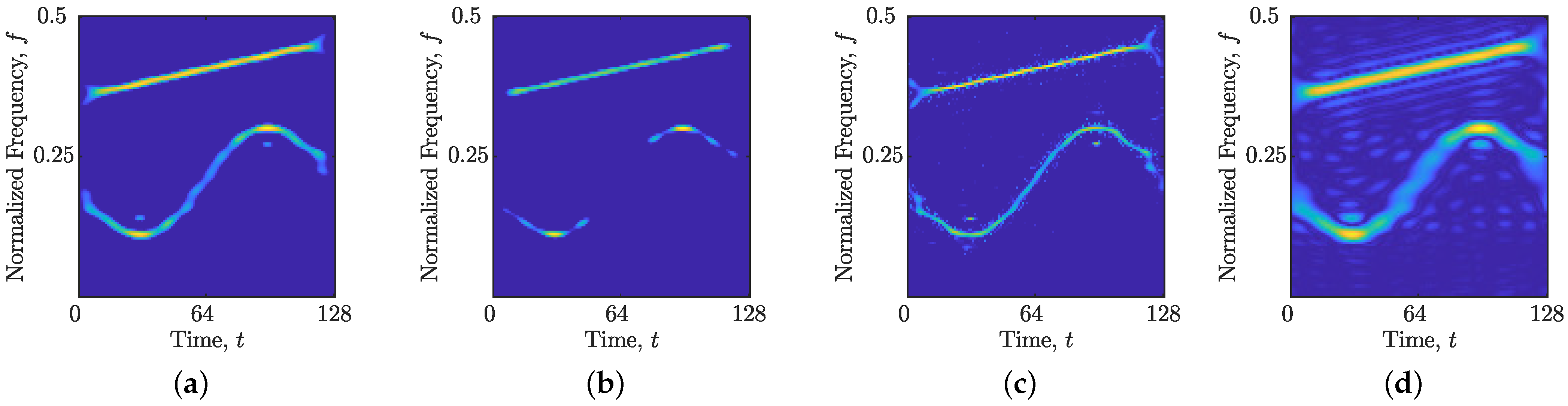
where the signal length is samples. Figure 1 portrays four reconstructed TFDs derived using the TwIST algorithm with a varying regularization parameter . The values were specifically chosen to highlight their impact on reconstruction performance: a high (Figure 1b) resulted in an overly sparse TFD with the SFM component absent, a low (Figure 1d) yielded a blurred TFD with substantial cross-term interference, and intermediate values (Figure 1a,c) produced TFDs with retained auto-terms, albeit with varying degrees of resolution and cross-term contamination.
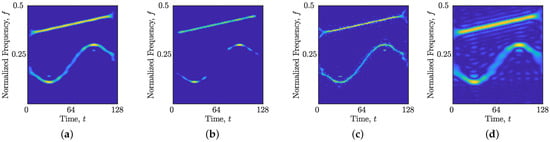
Figure 1.
Reconstructed TFDs for the signal obtained using the TwiST algorithm with , and (a) ; (b) ; (c) ; (d) .
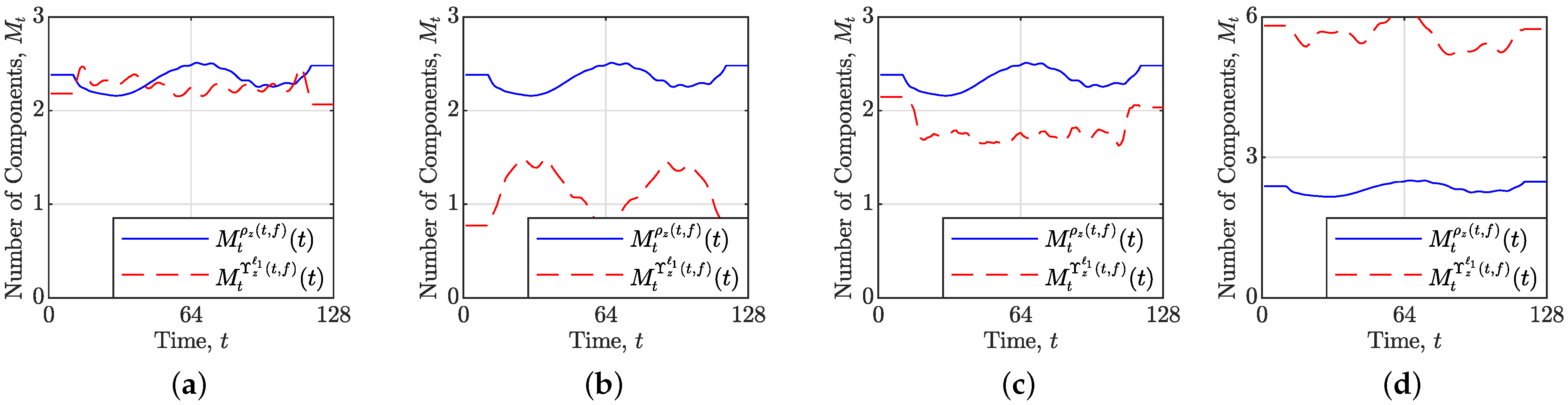
The LRE-based measure, as defined in (13) and (14), operates by comparing the local number of components estimated via LRE in the original and reconstructed TFDs. Figure 2 presents these LRE estimations for the corresponding TFDs in Figure 1. As expected, a loss of auto-terms is reflected in a decreased (Figure 2b), while the presence of interference or blurred auto-terms leads to an inflated relative to (Figure 2d).
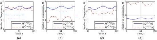
Figure 2.
Local number of components estimated from the starting TFDs (blue solid line) and reconstructed TFDs (dashed red line) for the signal obtained using the TwIST algorithm with and (a) ; (b) ; (c) ; (d) .
Despite its ability to circumvent the limitations of global measures and avoid favoring overly sparse TFDs, the LRE-based measure exhibits several inherent limitations.
Limitations Regarding Spatial Information: First, LRE fundamentally captures only one-dimensional information about auto-terms within the TFD, despite the inherent two-dimensional nature of the TF plane. This reduction in spatial information means that, for each time or frequency slice, the estimated local number of components only indicates the number of auto-terms, without specifying its precise location within that slice. This leads to a critical ambiguity: LRE cannot distinguish between a well-localized auto-term and a blurred, less informative representation. Moreover, LRE measures the entropy of the entire slice, regardless of whether the entropy originates from a single, concentrated energy atom or from a combination of a lower-resolution auto-term and cross-term artifacts. This is visually illustrated by comparing the TFDs in Figure 1a,c and their corresponding LRE estimations in Figure 2a,c. In this case, the estimated number of components is higher in time slices containing lower-resolution auto-terms compared to those with better-resolved auto-terms but also some cross-term contamination. This demonstrates that relying solely on LRE can lead to misinterpretations regarding the true quality of the reconstructed TFD.
Dependence on Reference Signal: Second, the LRE is inherently sensitive to the choice of reference signal. Prior research has demonstrated that the accuracy of LRE estimates diminishes when applied to components whose alignment deviates significantly from the reference signal [27]. While employing both and can partially mitigate this issue, consider two simple LFM components, and , which, despite their distinct time–frequency characteristics, yield identical LRE estimates: . This demonstrates a fundamental limitation in the ability of LRE to fully capture the nuances of different signal components.
Lack of Interpretability: Furthermore, the values, while normalized to the range as in [27], lack intrinsic interpretability. Table 1 presents the obtained values for the reconstructed TFDs in Figure 1. Based solely on these values, it is impossible to discern whether an increase in MSE stems from reconstructed interference, low-resolution auto-terms, or the complete loss of an auto-term. While access to the and curves could provide some additional insight, even this is not always conclusive. For instance, as illustrated in Figure 2c, a decrease in does not invariably indicate a loss of the auto-term. Consequently, the only reliable approach for discerning the true cause of the MSE value is to visually analyze the reconstructed TFD itself, which necessitates the storage and processing of potentially large data matrices, leading to memory inefficiency.

Table 1.
Evaluation of reconstructed TFDs obtained using the TwIST algorithm using the LRE-based metric for the considered synthetic signal .
Challenges for Automated Optimization: The aforementioned limitations pose significant challenges for automated systems, particularly meta-heuristic optimization algorithms tasked with identifying optimal parameter settings. Specifically, the conflicting nature of the optimization objectives in (15) exacerbates the problem. Efforts to minimize (i.e., drive the TFD towards an empty representation) can inadvertently lead to an increase in , hindering the algorithm’s ability to converge to a truly optimal solution.
In summary, these limitations—the loss of spatial information, the dependence on reference signals, the lack of interpretability in MSE values, and the challenges they pose for automated optimization—provide a compelling motivation for developing performance criteria that directly leverage the two-dimensional information inherent in auto-terms, as detailed in the subsequent section.
2.4. The Proposed Measure Based on the Instantaneous Frequency and Group Delay
The proposed measure aims to enhance TFD assessment by leveraging IF and GD estimations. In contrast to the LRE approach, which captures predominantly one-dimensional information, IF and GD estimations provide precise auto-term positioning within the two-dimensional TF plane. This enables a more comprehensive and nuanced evaluation based on three core criteria:
- Auto-Term Preservation: Quantifying the degree to which signal auto-terms are retained in the reconstructed TFD.
- Auto-Term Resolution: Assessing the sharpness and clarity of the reconstructed auto-terms.
- Interference Suppression: Measuring the effectiveness of suppressing cross-terms and noise artifacts.
Each criterion is quantified by a corresponding metric component: (auto-term preservation), (auto-term resolution), and (cross-term suppression).
2.4.1. Auto-Term Preservation ()
The auto-term preservation component, , evaluates the extent to which auto-terms are preserved in the TFD reconstruction. The approach involves analyzing each estimated IF and GD point to determine if a corresponding signal component is present within a defined neighborhood. For each estimated IF point, , corresponding to the -th signal component, the auto-term peak frequency, , is identified by searching for the first local maximum in the TFD amplitude within the frequency range that is closest to . The parameter defines a user-specified tolerance range, representing the maximum allowable deviation from the estimated IF within which a TFD value is considered a valid auto-term. The “first local maximum closest to” criterion is used to resolve cases where multiple maxima may be present within the tolerance range. An analogous procedure is applied for GD analysis. For each GD estimate, , the auto-term peak time, , is identified as the time of the first local maximum within the time range that is closest to .
If no positive maximum is detected within the specified range, it indicates a failure to preserve the auto-term, and is penalized by adding a value of 1. Otherwise, if an auto-term is detected, the value corresponding to the distance between and (or and ) is added to , calculated using a Gaussian function:
where is a user-defined tuning parameter that controls the width of the Gaussian function. A larger results in a wider Gaussian function, indicating a lower sensitivity to positional errors, while a smaller results in a narrower Gaussian function, indicating a higher sensitivity. This Gaussian weighting penalizes auto-terms that are located further away from their expected positions, reflecting a degradation in preservation accuracy. The parameter accounts for potential biases introduced by different TFDs and noise levels [13], while the Gaussian function offers a flexible mechanism for controlling the sensitivity to positional deviations. When the auto-term maximum coincides exactly with the estimated IF or GD (i.e., or ), , indicating no penalization. The final value of is computed as the mean of all computed values and is bounded within the range , where lower values indicate better auto-term preservation.
2.4.2. Auto-Term Resolution ()
The auto-term resolution component, , quantifies the sharpness and clarity of the reconstructed auto-terms within the TFD. Specifically, it calculates the mean width of the main lobe for each detected auto-term. For each auto-term, the frequency bins (or time samples) to the left and right of the auto-term maximum are identified at the points where the TFD amplitude decreases to of the maximum amplitude. This threshold corresponds to the −3 dB point, commonly used in signal processing to define the effective bandwidth or main lobe width [40]. These points establish the boundaries of the main lobe. The width of the main lobe is then normalized by either or , depending on whether the auto-term was identified using IF or GD estimates, respectively. This normalization ensures that is interpretable across different TFD dimensions.
Unlike previous approaches that rely on normalized instantaneous bandwidth [40], this method provides a direct measure of the spatial extent of the auto-term in the TF plane. The resulting value is bounded within the range , where smaller values indicate higher resolution (i.e., sharper auto-terms). The ideal auto-term resolution occurs when the auto-term occupies only a single sample or bin, resulting in .
2.4.3. Interference Suppression ()
The interference suppression component, , evaluates the effectiveness of suppressing cross-terms and noise artifacts within the TFD. To calculate this metric, the identified auto-terms are first removed from the TFD. The remaining samples are then considered to be primarily composed of cross-terms and noise. The metric is then calculated as
where represents the norm, which counts the number of non-zero elements in the TFD after auto-term removal. The result is then normalized by the total number of samples in the TFD (). Consequently, can be interpreted as the percentage of the TFD energy that is attributed to cross-terms and noise. This metric is bounded between , where lower values indicate better cross-term suppression. An ideal value of indicates that all interference terms have been completely eliminated from the TFD.
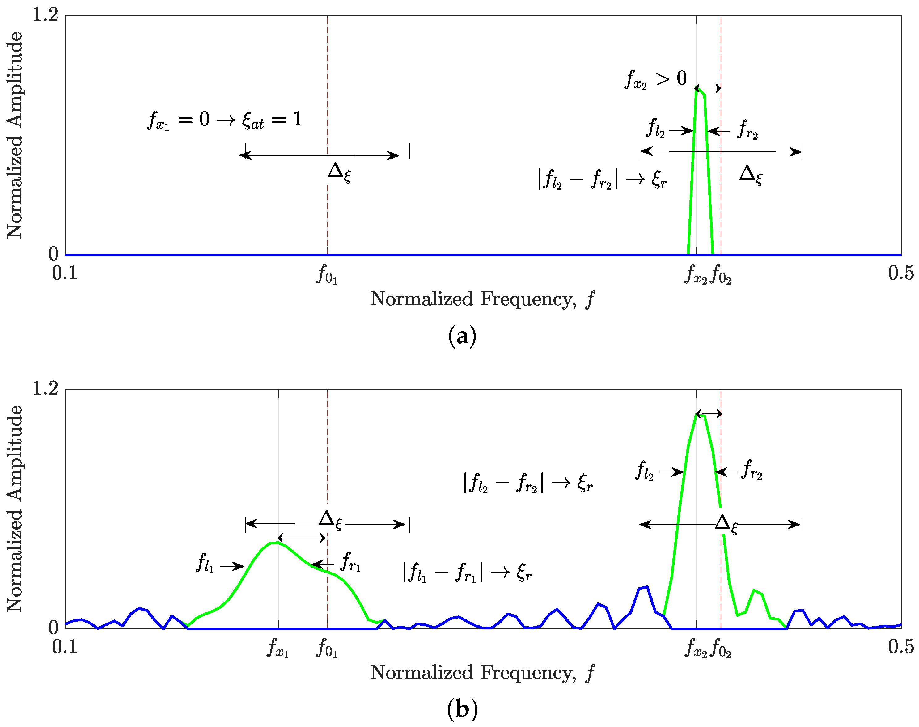
Figure 3 provides an illustrative example of the proposed measure applied to time slices of reconstructed TFDs for the signal . Figure 3a depicts a time slice from an overly sparse TFD. For the first estimated IF, , no auto-term is detected within the tolerance range, resulting in a penalty of 1 for . For the second estimated IF, , an auto-term is detected, and the corresponding value is calculated using (18). The resolution of this auto-term is then assessed as . Since the TFD is overly sparse, . Conversely, Figure 3b illustrates a time slice from a TFD reconstructed with a low regularization parameter (), leading to low-resolution auto-terms and substantial interference. While both auto-terms are detected, their resolution is lower than in Figure 3a. Furthermore, this time slice contains a significant number of interference components, resulting in a higher value compared to the time slice in Figure 3a.
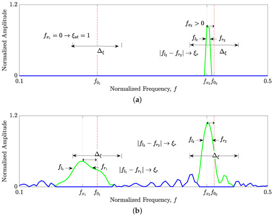
Figure 3.
Illustrative example of the proposed measure applied to time slices of reconstructed TFDs of signal : (a) time slice from an overly sparse TFD, illustrating a missing auto-term; (b) time slice from a TFD with low regularization, showing low-resolution auto-terms and reconstructed interference. The green lines represent signal auto-terms, while the blue lines represent regions classified as interference.
2.4.4. Component Alignment Map Integration
To automate the selection of appropriate IF and GD estimates for TFD analysis, the proposed measure leverages the CAM, as introduced in [29]. CAM automatically determines TFD regions where localization is best performed using time slices (i.e., IF analysis) or frequency slices (i.e., GD analysis). CAM analysis exploits the fact that LRE estimates artificially increase when a component’s alignment deviates significantly from the reference signal, suggesting the need for an alternative localization approach. The CAM method extracts TFD segments where such increases occur and then applies connectivity analysis to identify discontinuous component estimates resulting from unsuitable localization approaches [29]. The CAM generates a binary map, where indicates TFD regions where localization in time slices (IF analysis) is preferred, and indicates regions where localization in frequency slices (GD analysis) is preferred. In the context of the proposed measure, CAM facilitates automatic selection of IF or GD estimates based on the local characteristics of the TFD.
2.4.5. Multi-Objective Optimization
Furthermore, the proposed measure components, , , and , can serve as objective functions to be minimized within a multi-objective optimization framework, analogous to the approach described in (15):
A key advantage of the proposed measure components is that they are not inherently conflicting, unlike the LRE-based objective functions in (15). For example, achieving a minimal , signifying perfect auto-term preservation with accurate positioning, does not necessarily imply an increase in or . This property facilitates more robust and efficient optimization, as the algorithm can independently optimize each component without being constrained by inherent trade-offs.
2.4.6. Summary of the Proposed Performance Measure
The key steps of the proposed measure can be summarized as follows:
- Initialization: Initialize the auto-term preservation () and auto-term resolution () components to zero.
- IF Analysis (Time Slices): For each estimated IF point where , search for the auto-term maximum within the corresponding time slice.
- Auto-Term Preservation Assessment: If no positive maximum is detected within the tolerance range, increment by 1 to penalize the lack of auto-term preservation. Skip steps 4 and 5. Otherwise, increment based on the distance between the estimated IF and the detected auto-term maximum, calculated using the Gaussian function in (18).
- Auto-Term Resolution Assessment: Locate the frequency bins to the left and right of the detected auto-term maximum where the TFD amplitude is equal to of the maximum value. Increment with the width of this frequency range.
- Auto-Term Removal: Remove the considered auto-term from the TFD in a local neighborhood around the detected auto-term maximum.
- GD Analysis (Frequency Slices): Repeat steps 2–5 for each estimated GD point where , using frequency slices.
- Normalization: Normalize by the total number of estimated IF and GD points, and normalize by the total number of detected auto-term maxima.
- Interference Suppression Assessment: After removing all identified auto-terms, determine the amount of interference by calculating the number of non-zero elements in the remaining TFD using (19).
3. Experimental Results and Discussion
To evaluate the performance of the proposed measure, a series of experiments were conducted using both synthetic and real-world signals. The synthetic signals allowed for controlled assessment of the measure’s sensitivity to various signal parameters and noise levels, while the real-world signal provided insight into its applicability in practical scenarios.
3.1. Selection of the Signal Examples
The performance of the proposed measure was evaluated using three synthetic signals. The first signal, with samples, is defined in (17). The second signal, with samples, consists of four time-limited LFM components with different amplitudes embedded in AWGN with dB:
Here, the rectangular function is defined as , where , , and denote the starting time, ending time, and duration of the signal component, respectively. The introduction of time-limited components and AWGN simulates more realistic signal conditions and allows for assessing the measure’s robustness to noise and interference. The third signal, with samples, comprises two quadratic frequency-modulated (QFM) components:
In addition to the synthetic signals, a real-world gravitational wave signal (this research has made use of data, software, and/or web tools obtained from the LIGO Open Science Center (https://losc.ligo.org (accessed on 17 February 2025)), a service of LIGO Laboratory and the LIGO Scientific Collaboration. LIGO is funded by the U.S. National Science Foundation), [28,41,42], denoted as , was included in the evaluation. To prepare the signal for analysis, established pre-processing techniques were employed, including downsampling the original signal by a factor of 14, resulting in samples, corresponding to a duration of 0.25 to 0.45 s and a frequency range of Hz. This downsampling procedure is consistent with prior work and serves to reduce computational complexity without significantly compromising the essential signal characteristics [28].
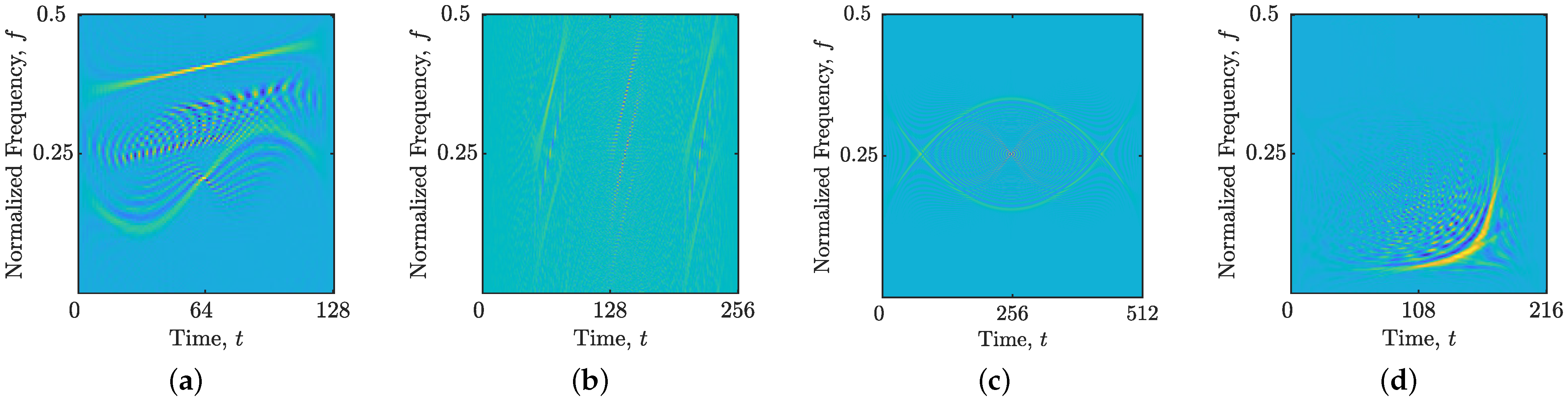
Figure 4 illustrates the WVDs of the considered signals , , , and . It is evident from these figures that the WVDs are characterized by significant cross-term interference (and noise for ), due to the lack of any filtering. These artifacts underscore the need for effective cross-term suppression techniques, such as the CS-based approach employed in this study.
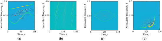
Figure 4.
WVDs of the considered synthetic and real-world gravitational signals: (a) ; (b) ; (c) ; (d) .
3.2. Parameter Settings and Computational Resources
The calculation of the LRE involved the following parameters: and , consistent with recommendations in prior literature [31,43]. The CS-AF areas for the signals , , , and were determined to be , , , and , respectively, using the approach detailed in [26]. The tolerance level for the reconstruction algorithm was set to , as in [19,26,27,28]. For meta-heuristic optimization, the MOPSO algorithm was employed with parameter settings as specified in [27].
The proposed measure’s parameters, and , were optimized for each synthetic signal by minimizing the -norm between the reconstructed TFD, , and an ideal reference TFD, , when optimizing with MOPSO. The ideal reference TFDs were generated based on the true IF and GD trajectories of the signals. The optimized values were found to be and . The -norm is calculated as
The simulations of the algorithms’ execution times, averaged over 1000 independent runs, have been performed on a PC with the Ryzen 7 3700X @ 3.60 GHz Base Clock processor and 32 GB of DDR4 RAM.
3.3. Component Alignment Maps and IF/GD Estimates
Figure 5 and Figure 6 depict the CAMs and estimated GDs and IFs for the signals, respectively. These estimates were derived using a blind source separation algorithm and an automatic IF and GD estimation method as detailed in [29]. As illustrated, signals and are well suited for localization through time slices, while signal is better suited for localization through frequency slices. The gravitational wave signal, , exhibits characteristics that necessitate both time and frequency localizations, highlighting the adaptability of the proposed measure.

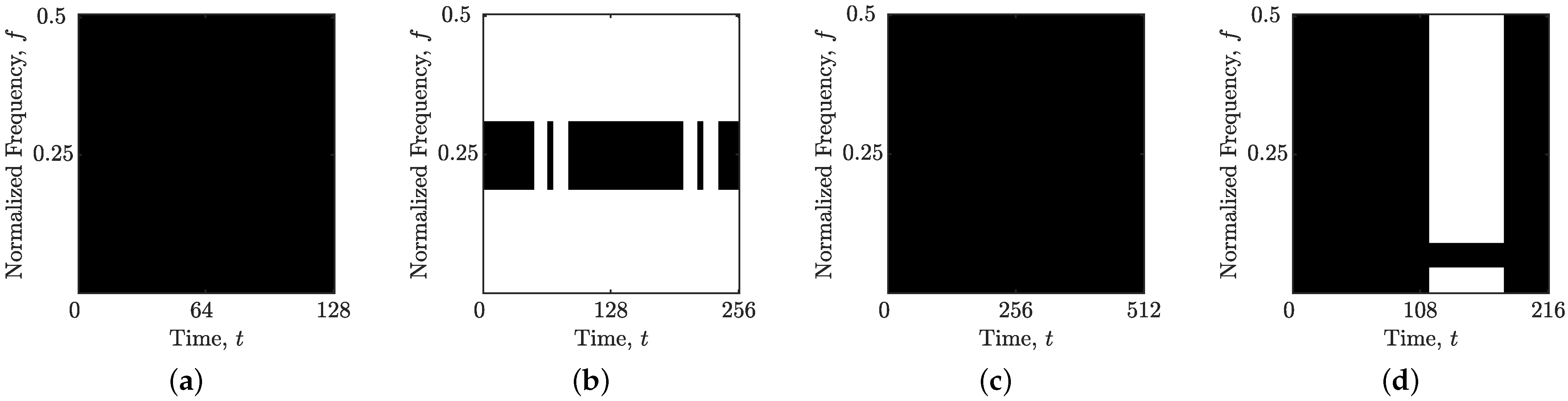
Figure 5.
Obtained CAMs of the considered synthetic and real-world gravitational signals: (a) ; (b) ; (c) ; (d) . TFD regions in black indicate that localization in time slices in preferred containing IFs, while regions in white indicate that localization in frequency is preferred containing GDs.
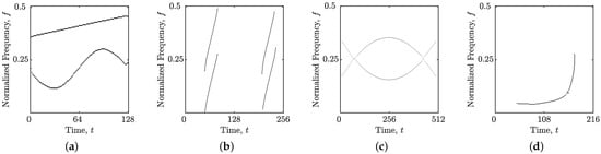
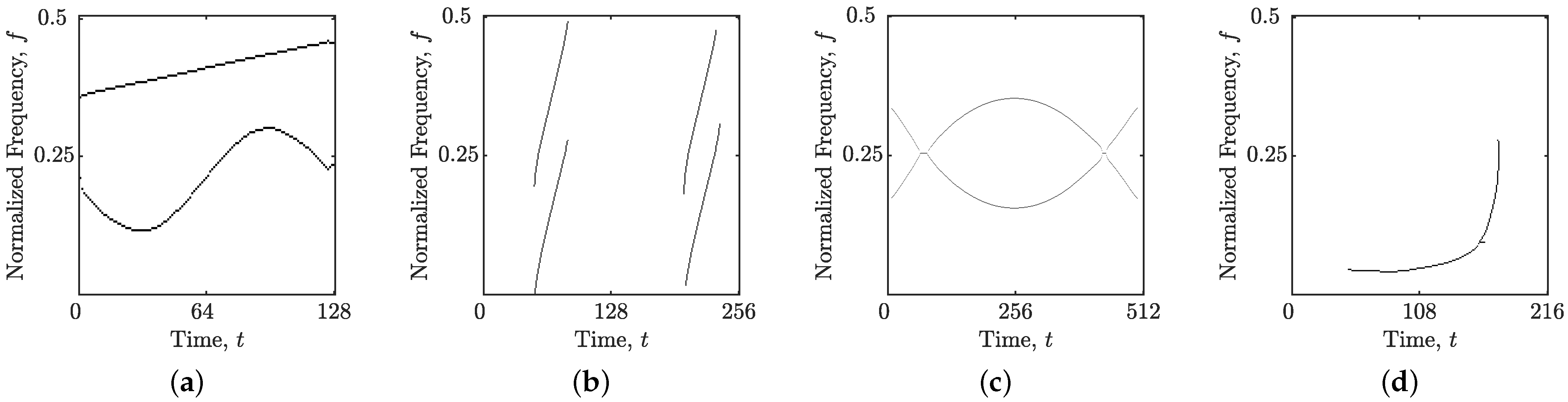
Figure 6.
Estimated IFs and GDs of the considered synthetic and real-world gravitational signals: (a) ; (b) ; (c) ; (d) .
3.4. Results: Synthetic and Real-World Signals
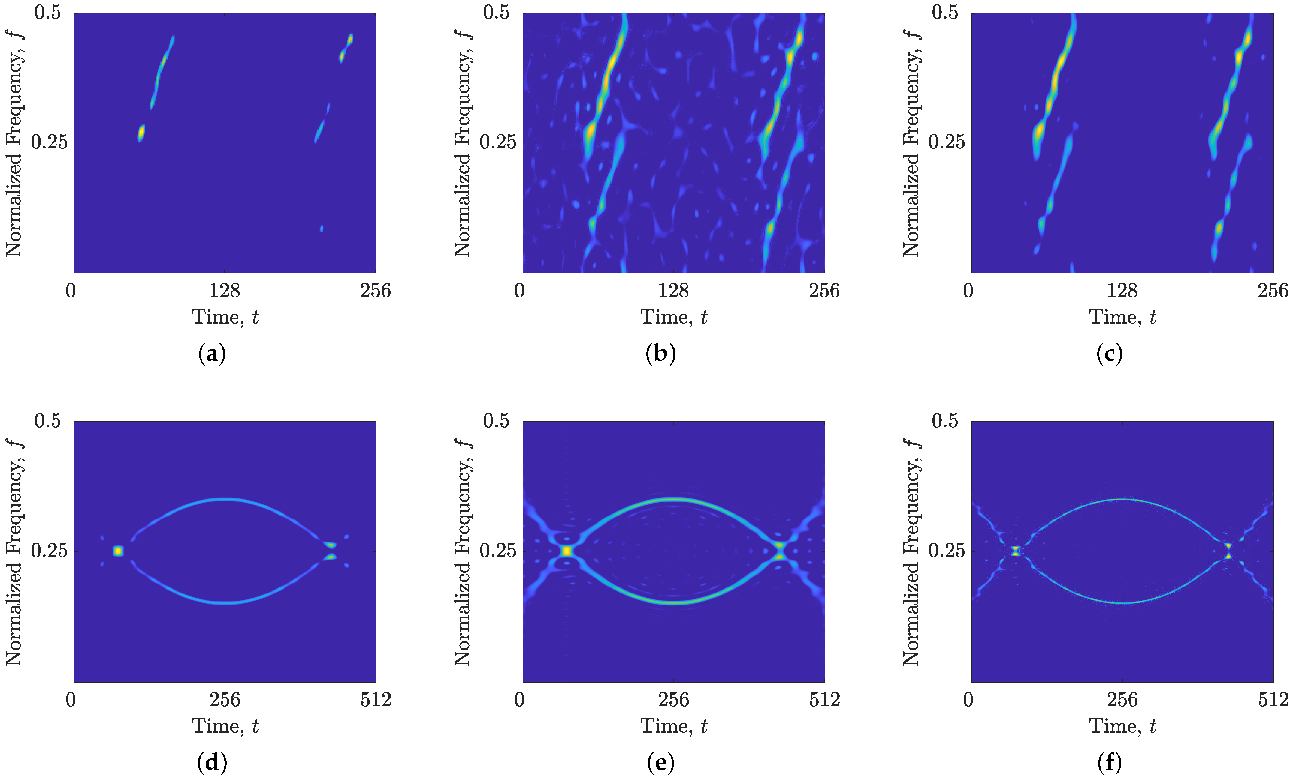
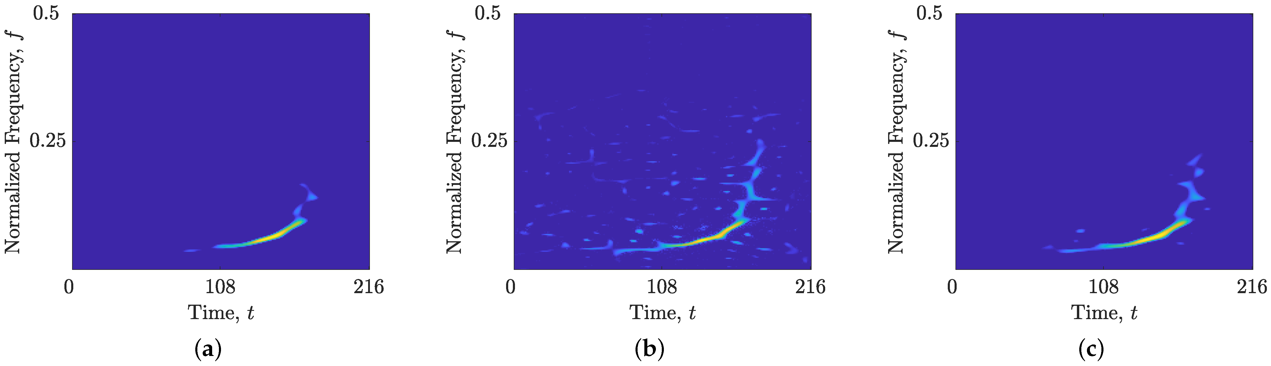
The reconstructed TFDs for the experimental tests were generated using the TwIST algorithm with distinct values to represent different reconstruction outcomes. Case 1 utilized a high parameter, resulting in significant auto-term loss. Case 2 employed values that led to unsuccessful reconstructions dominated by interference. Case 3 TFDs were generated with values between those of Cases 1 and 2, achieving a balance of improved auto-term preservation and reduced interference. Figure 7 illustrates these reconstructed TFDs for all considered signals across Cases 1–3, while Table 2 presents a comparative analysis of the proposed measure against existing measures in evaluating the reconstructed TFD performance.
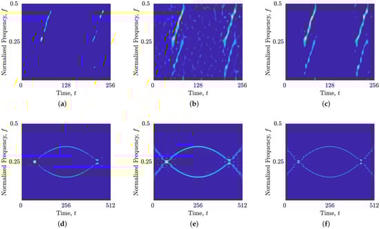
Figure 7.
Reconstructed TFDs of the synthetic signals obtained using the TwIST algorithm with , , and: (a) , (Case 1); (b) , (Case 2); (c) , (Case 3); (d) , (Case 1); (e) , (Case 2); (f) , (Case 3).
Table 2.
Performance comparison of reconstructed TFDs obtained using the TwIST algorithm for the synthetic signals , and . Values in bold indicate superior reconstructed TFD for each measure.
The results, based on the -norm, indicate that the Case 3 reconstructed TFDs consistently provide a closer approximation to the ideal TFDs than those in Cases 1 and 2 across all signal examples. In line with prior research [27], the global measures and R tend to favor overly sparse TFDs, incorrectly identifying Case 1 as optimal due to their inherent disregard for crucial auto-term information. For signals and , the LRE-based metric effectively penalizes the TFDs in Cases 1 and 2, assigning them higher error values and correctly identifying the reconstructed TFD in Case 3 as the best performing. However, this trend does not hold for signal , where erroneously identifies the overly sparse reconstructed TFD in Case 1 as optimal. It is important to note that values were not computed for the WVD due to two primary reasons: first, LRE is typically applied to QTFDs where interference is mitigated; and second, the appropriate reference TFD for the WVD would also be a WVD, which is inherently incomparable to the reference TFDs used for the reconstructed TFDs.
In contrast, the proposed measure components offer more nuanced insights into TFD performance. Across all signal examples, indicates that the WVD and the reconstructed TFDs in Case 2 retain all auto-terms, while the reconstructed TFDs in Case 3 exhibit superior performance compared to those in Case 1. Furthermore, effectively identifies the TFDs with the highest auto-term resolution, with the reconstructed TFDs in Case 3 surpassing those in Case 2, which suffer from poor resolution. As for , it accurately identifies the overly sparse TFDs as free from both interference and noise artifacts, a characteristic not shared by the WVD. It also confirms that the reconstructed TFDs in Case 3 demonstrate a lower degree of unsuppressed interference compared to those in Case 2. Consequently, when the proposed measure components are equally averaged, the reconstructed TFDs in Case 3 are consistently identified as the best performing for all three signal examples.
These observations concerning the measures’ performance in evaluating reconstructed TFDs extend to the real-world gravitational signal . Figure 8 illustrates the Case 1–3 reconstructed TFDs for this signal, while Table 3 presents the corresponding performance results. Consistent with the trends observed for the synthetic signals, the and R measures favor overly sparse TFDs, and the measure incorrectly identifies the corrupted reconstructed TFD in Case 2 as the best performing. The proposed measure component highlights the WVD as having full retention of auto-terms. However, in contrast to the synthetic signals, reveals that the reconstructed TFDs in Case 2 are missing several auto-term samples. This discrepancy arises from the limitations of the rectangular CS-AF area, which fails to adapt its vertices appropriately for higher-order FM components present in signal [28]. The component correctly identifies the overly sparse reconstructed TFDs in Case 1 as exhibiting the best auto-term resolution and minimal interference. In summary, the averaged proposed measure components accurately demonstrate that the reconstructed TFDs in Case 3 offer the best overall performance among the tested cases.
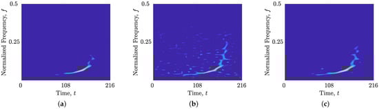
Figure 8.
Reconstructed TFDs of the real-world gravitational signal obtained using the TwIST algorithm with , , and (a) (Case 1); (b) , (Case 2); (c) , (Case 3).
Table 3.
Performance comparison of reconstructed TFDs obtained using the TwIST algorithm for the real-world gravitational signal . Values in bold indicate superior reconstructed TFD for each measure.
3.5. Meta-Heuristic Optimization Comparison
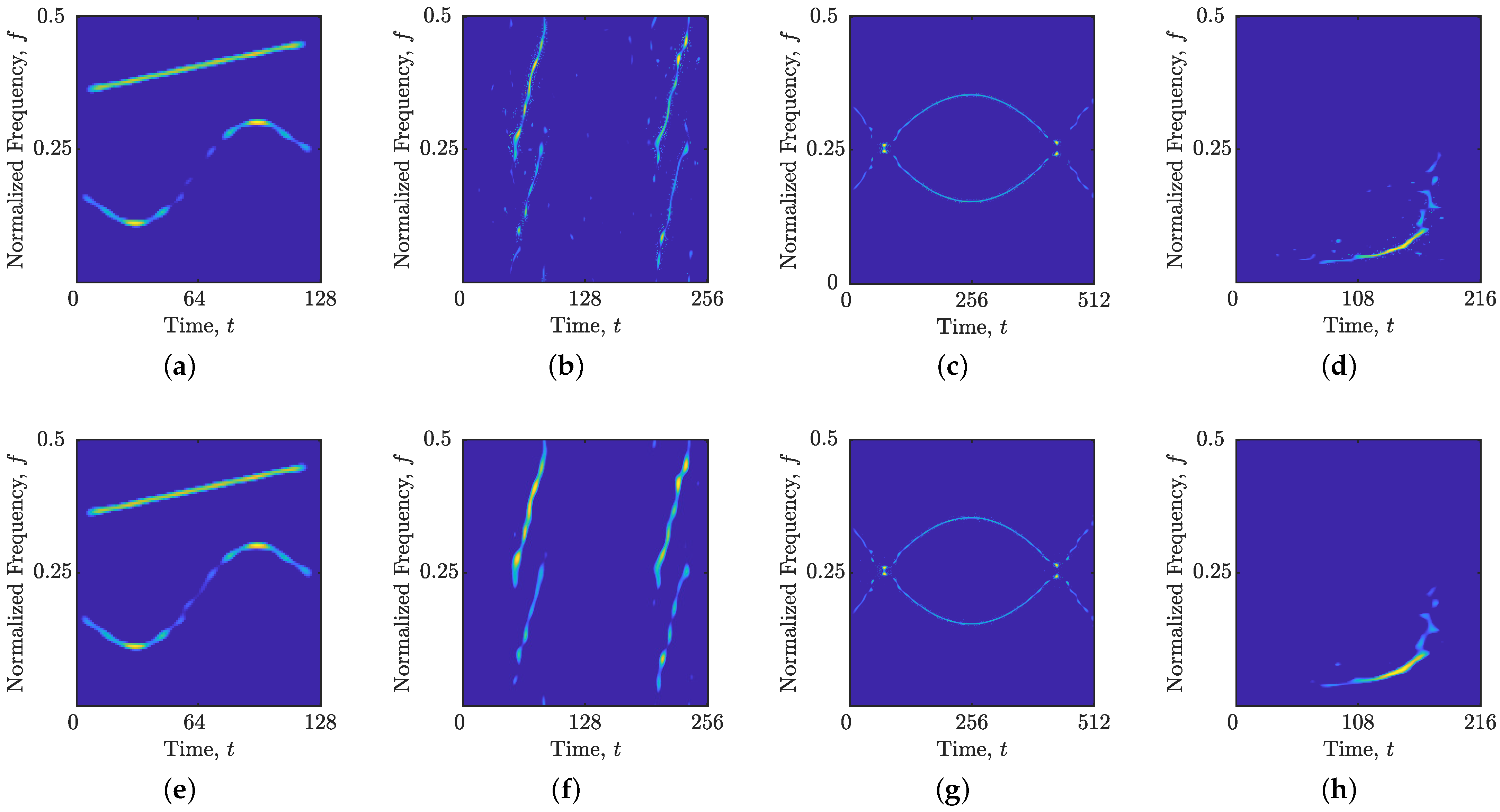
Figure 9 presents a visual comparison of optimized reconstructed TFDs obtained using MOPSO with two distinct sets of objective functions: the proposed measures and the existing measures. Table 4 and Table 5 provide a corresponding numerical comparison.
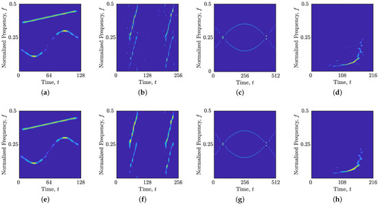
Figure 9.
Optimized reconstructed TFDs of the considered synthetic and real-world gravitational signals obtained using the TwIST algorithm and MOPSO with the following objective functions: (a) , , ; (b) , , ; (c) , , ; (d) , , ; (e) , , ; (f) , , ; (g) , , ; (h) , , .
Table 4.
Performance comparison of reconstructed TFDs obtained using the TwIST algorithm and MOPSO for the synthetic signals , and . Values in bold indicate superior reconstructed TFD for each measure.
Table 5.
Performance comparison of reconstructed TFDs obtained using the TwIST algorithm and MOPSO for the real-world gravitational signal . Values in bold indicate superior reconstructed TFD for each measure.
The results indicate that optimization with the proposed measures consistently yields reconstructed TFDs with well-preserved auto-terms, high resolution, and suppressed interference. Furthermore, the proposed measures led to a consistent improvement in optimized reconstructed TFDs for all considered signals compared to the results obtained using . Specifically, the -norm, a measure of the deviation from an ideal TFD, was improved by 3.68% to 65.10%, demonstrating the superior ability of to generate reconstructed TFDs that closely approximate the ideal.
It is important to note that for all considered signals, the proposed measures resulted in better preservation of auto-terms, as evidenced by consistently lower values. While the objectives sometimes yielded slightly higher auto-term resolution (higher ), this improvement often came at the cost of losing essential parts of the auto-terms (see Figure 9a,c). For the noisy signals and , the objectives resulted in lower values, indicative of less effective interference suppression (see Figure 9b,d), as confirmed by generally worse values, except in the case of .
Finally, the time required to achieve optimized reconstructed TFDs using the proposed objectives was significantly reduced, ranging from 44.17% to 60.63%, compared to the time required for the existing objectives. This reduction in computational cost highlights the efficiency of the proposed measure for meta-heuristic optimization.
3.6. Noise Sensitivity Analysis
To further evaluate the robustness of meta-heuristic optimization using the proposed objective functions, synthetic signal examples were embedded in AWGN at SNR levels ranging from 0 dB to 9 dB. The results, summarized in Table 6, demonstrate a consistent improvement when using the proposed measures over the existing measures across all tested SNR levels.
Table 6.
Performance comparison of reconstructed TFDs obtained using the TwIST algorithm and MOPSO for synthetic signals , and embedded in AWGN in SNR dB. Values in bold indicate superior reconstructed TFD based on the metric.
Specifically, the -norm, a measure of the deviation from the ideal TFD, was improved by 16.26% at 0 dB SNR, 61.06% at 3 dB SNR, 57.67% at 6 dB SNR, and 51.79% at 9 dB SNR. This indicates that the proposed objective functions lead to more accurate TFD reconstructions, even in the presence of significant noise.
Furthermore, the results suggest that the performance degradation due to decreasing AWGN SNR levels is less pronounced when optimizing with the proposed objectives compared to the objectives. This highlights the superior noise resilience of the proposed approach.
3.7. Interpretation of the Results
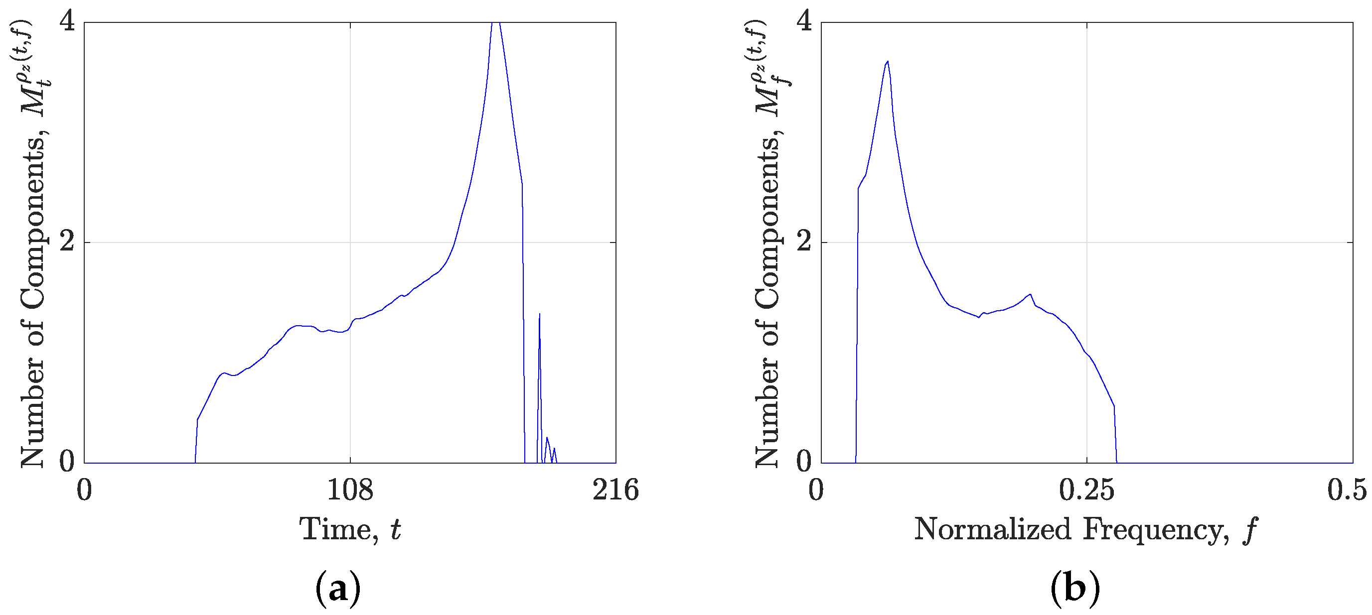
As shown in [27], global measures and R tend to favor overly sparse TFDs (Case 1) for all signal examples, limiting their applicability when auto-term preservation is a priority. While the LRE-based metric successfully penalizes the reconstructed TFDs in Cases 1 and 2 with higher error values for signals and , its performance is inconsistent for signals and . This stems from the LRE limitation when analyzing intersecting components, as in signal , where a drop in the estimated local number of components leads to favoring overly sparse TFDs. In the case of signal , Figure 10 illustrates that the hyperbolic behavior of the signal’s auto-term makes it unsuitable for LRE localization. Specifically, both LRE estimations exhibit an artificial increase when the component changes its slope with respect to the time or frequency axis, causing to favor the corrupted reconstructed TFD in Case 2.
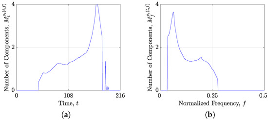
Figure 10.
Local number of components estimated from the starting TFDs for the signal : (a) ; (b) .
Such misclassifications can confuse end-users when selecting the best-performing reconstructed TFD. Furthermore, even when the LRE-based measure provides a correct assessment, it lacks the interpretability needed to guide the adjustment of the parameter. Instead, users must analyze the relationship between the and curves to infer the presence of over-sparsity or interference. However, this analysis can be ambiguous, especially when the number of local components increases post-reconstruction, resulting in a higher curve compared to . This discrepancy can stem from low-resolution auto-terms or the reconstruction of cross-terms and noise, yet the precise cause remains elusive.
Conversely, the proposed measure components provide clearer insights than the LRE metric. For instance, a low combined with a high suggests well-preserved auto-terms with reduced resolution. A significantly high , indicates interference in the reconstructed TFDs, suggesting that is set too low (as in Case 2 with ). Conversely, a high with very low and points to an overly sparse reconstructed TFD with inconsistent auto-terms, implying that is set too high (as in Case 1). In both scenarios, the proposed measures offer guidance on whether should be increased or decreased, providing a distinct advantage over the existing LRE-based metric used in [27]. The capacity to decouple , , and is a particular advantage since that enables an unambiguous interpretation of the result.
Quantitatively, a of 0.0056 for Case 3’s reconstructed TFD for signal signifies a very high resolution of auto-terms, averaging just two samples per estimated IF. Also, a of 0.4149 for Case 2’s reconstructed TFD for signal signifies that 41.49% of the TFD (of size ) is corrupted by interference. These quantitative indicators directly enhance the interpretability of the proposed measure.
In addition to the increased interpretability, the findings demonstrate that the proposed measure components, when averaged equally, successfully highlight the best-performing reconstructed TFD. These findings and conclusions drawn from the synthetic signals also extend to the real-world gravitational signal. The various presented signal examples with multiple LFM and QFM components, with varying amplitudes and intersecting cases, demonstrate the robustness and suitability of the proposed measure for a wide range of signals.
When implementing the proposed measure components in meta-heuristic optimization, the results shown in Table 4 and Table 5 illustrate that reconstructed TFDs optimized using the proposed measure’s components exhibit well-preserved auto-terms and suppressed interference. Even though optimizing with the LRE-based measure can lead to reconstructed TFDs with preserved auto-terms and less interference, the usage of the proposed measures further improves optimization performance. To complement these results, Table 6 indicates a meta-heuristic optimization improvement in noisy environments, where reconstructed TFDs optimized using the proposed measure’s components proved to be better than those obtained using the LRE-based measure across all considered SNR levels. This highlights the proposed measure over the existing LRE-based measure in noisy environments, where the limitations of the LRE are pronounced.
Even though the CS-based TFD reconstruction method is typically considered for offline analysis, the results illustrate that the proposed measure is beneficial for optimizing TFD, as the optimization time is significantly reduced by using the proposed measures as objective functions. The reasons for this are twofold. Firstly, the proposed measures are not as conflicted as and . Secondly, can yield the same increased value for both overly sparse TFDs (high ) and TFDs with interference (low ), which confuses and slows the convergence of meta-heuristics. While memory efficiency for storing information is not always a primary concern in this field, it is important to consider the memory requirement associated with different approaches. Storing values alongside the corresponding measures provides a comprehensive understanding of the impact of on TFD performance. Analyzing the existing measures in a similar way would necessitate substantially greater memory resources, as it would involve storing not only but also the vectors from both the original and reconstructed TFDs, and in many cases, the full reconstructed TFDs. The memory would increase significantly, potentially reaching hundreds of megabytes.
The inclusion of CAM in the proposed measure enables the automatic selection of IF and GD estimates, circumventing the need for manual selection of time and frequency localization. Therefore, users are not required to manually identify and separate the components best suited for localization via time or frequency slices, which increases the overall convenience of the method. However, it should be noted that, by its very construction, the inclusion of CAM and a mandatory matrix with IF and/or GD estimates indicates that the proposed measure requires more inputs than the LRE.
The selection of the LRE method should be discussed. This study uses the original LRE approach, which was established in LRE-based measures in [27,28]. This original approach was robust and applicable to a different set of signals. An iterative LRE approach proposed in [44] may be used in special cases of signals comprising multiple components with significant differences in amplitudes. However, the iterative LRE implies several other limitations, such as incorrect component removal for intersecting components and significantly higher sensitivity to noise, making this approach applicable only for special cases. A study in [45] circumvented some limitations of the original and iterative LRE approach by using convolutional neural networks. This involves neural networks trained using a diverse dataset of signals to predict the local number of components from an input QTFD. This study did not utilize that approach for two reasons. Firstly, the network is trained on QTFDs, meaning that it can predict local numbers of components for a starting TFD, but not for a reconstructed TFD. This would require retraining the network on this specific task. Secondly, estimates provided by the network are very volatile, and research on applying some smoothing filters is still required before usage.
The optimization of and parameters relies on numerical simulations in sparse TFD reconstructions. Furthermore, for overall evaluation, the measured components have been averaged for overall interpretation, meaning that all three components have equal importance. Users are encouraged to retest parameters and and pronounce the importance of some measured components if they find them beneficial in specific TFD or advanced methods.
The enhanced assessment of reconstructed TFDs using the proposed measure has significant potential in this field. The improvement is demonstrated through the interpretability of the proposed measure when compared to the existing methods. This opens up many research directions in machine-related applications.
4. Conclusions
CS-based methods have emerged as powerful tools for generating high-performing TFDs. However, a critical challenge remains: the potential loss of auto-terms during reconstruction, which hinders accurate TFD assessment and the selection of optimal reconstruction parameters. The existing measure, which is based on the LRE, addresses some of these limitations, but it also exhibits shortcomings.
This study addresses these challenges by presenting a novel performance measure for evaluating TFD reconstruction quality, with a specific focus on robust auto-term preservation. By incorporating IF and GD estimates directly within the 2D TF plane, the proposed measure offers a comprehensive and nuanced assessment of reconstructed TFDs. This assessment is based on three key, decoupled components: auto-term preservation (), which quantifies the retention of signal components; auto-term resolution (), which measures the sharpness and clarity of the reconstructed components; and cross-term suppression (), which evaluates the effectiveness in reducing interference and noise artifacts.
Experimental results, obtained from a diverse set of synthetic signals (encompassing linear and non-linear FM components, intersecting components, and components with varying amplitudes in noise) and real-world gravitational wave data, demonstrate the effectiveness of the proposed metric in detecting common reconstruction issues. Notably, unlike previous LRE-based metrics, the proposed measure reliably distinguishes between overly sparse TFDs and those contaminated by interference, enabling users to gain valuable insights for fine-tuning reconstruction parameters and improving TFD quality.
This study further demonstrates that, when integrated into an automated meta-heuristic optimization framework, the proposed metric significantly enhances the quality of TFDs, leading to improved auto-term preservation and reduced interference, even under challenging noisy conditions. Moreover, the optimized reconstructed TFDs were obtained significantly faster using the proposed measure as objective functions, highlighting its computational efficiency. Also, the regularization parameter can be stored more efficiently by relying only on the proposed measure’s values, rather than the memory-inefficient TFDs, highlighting its practical application.
These findings underscore the significant value of the proposed metric not only for individual users seeking to improve TFD reconstruction but also for machine-driven applications that require an interpretable, reliable, and computationally efficient measure of TFD quality. Given its effectiveness and efficiency, the proposed measure can serve as a valuable feature extraction function for future research directions in deep learning applications.
Funding
This research was funded by University of Rijeka, Croatia; grant number: uniri-mladi-tehnic-23-2 (Analysis of non-stationary signals using time-frequency algorithms and deep learning).
Data Availability Statement
The data presented in this study are available on request from the corresponding author.
Conflicts of Interest
The author declares no conflicts of interest.
Abbreviations
The following abbreviations are used in this manuscript:
| AF | Ambiguity function |
| AWGN | Additive white Gaussian noise |
| CS | Compressive sensing |
| CAM | Component alignment map |
| ECM | Energy concentration measure |
| FM | Frequency modulation |
| FSM | Fuzzy satisfying method |
| FT | Fourier transform |
| GD | Group delay |
| IF | Instantaneous frequency |
| LFM | Linear frequency modulation |
| LIGO | Laser interferometer gravitational-wave observatory |
| LRE | Localized Renyi entropy |
| MOPSO | Multi-objective particle swarm optimization |
| MSE | Mean squared error |
| QFM | Quadratic frequency-modulation |
| QTFD | Quadratic time–frequency distribution |
| SFM | Sinusoidal frequency modulation |
| SNR | Signal-to-noise ratio |
| TF | Time–frequency |
| TFD | Time–frequency distribution |
| TwIST | Two-step iterative shrinkage/thresholding |
| WVD | Wigner–Ville distribution |
References
- Liu, N.; Gao, J.; Zhang, B.; Li, F.; Wang, Q. Time–Frequency Analysis of Seismic Data Using a Three Parameters S Transform. IEEE Geosci. Remote Sens. Lett. 2018, 15, 142–146. [Google Scholar] [CrossRef]
- Yi, X.; Yang, S.; Dong, R.; Ren, Q.; Shuai, T.; Li, G.; Gong, W. A composite clock for robust time-frequency signal generation system onboard a navigation satellite. GPS Solut. 2023, 28, 6. [Google Scholar] [CrossRef]
- Wu, D.; Yang, Z.; Ruan, Y.; Chen, X. Blind single-channel lamb wave mode separation using independent component analysis on time-frequency signal representation. Appl. Acoust. 2024, 216, 109810. [Google Scholar] [CrossRef]
- Song, Y.; Hu, Y.; Chen, X.; Chen, H.; Zhang, P. Time-Reassigning Transform for the Time–Frequency Analysis of Seismic Data. IEEE Trans. Geosci. Remote Sens. 2024, 62, 4505811. [Google Scholar] [CrossRef]
- Song, K.; Nie, J.; Li, Y.; Li, J.; Song, P.; Ercisli, S. Regional soil water content monitoring based on time-frequency spectrogram of low-frequency swept acoustic signal. Geoderma 2024, 441, 116765. [Google Scholar] [CrossRef]
- Lekkas, G.; Vrochidou, E.; Papakostas, G.A. Time–Frequency Transformations for Enhanced Biomedical Signal Classification with Convolutional Neural Networks. BioMedInformatics 2025, 5, 7. [Google Scholar] [CrossRef]
- Adamczyk, K.; Polak, A.G. Online Algorithm for Deriving Heart Rate Variability Components and Their Time–Frequency Analysis. Appl. Sci. 2025, 15, 1210. [Google Scholar] [CrossRef]
- Zhang, H.; Wu, Q.; Tang, W.; Yang, J. Acoustic Signal-Based Defect Identification for Directed Energy Deposition-Arc Using Wavelet Time–Frequency Diagrams. Sensors 2024, 24, 4397. [Google Scholar] [CrossRef]
- Łuczak, D. Data-Driven Machine Fault Diagnosis of Multisensor Vibration Data Using Synchrosqueezed Transform and Time-Frequency Image Recognition with Convolutional Neural Network. Electronics 2024, 13, 2411. [Google Scholar] [CrossRef]
- Wei, M.; Sun, X.; Zong, J. Time–Frequency Domain Seismic Signal Denoising Based on Generative Adversarial Networks. Appl. Sci. 2024, 14, 4496. [Google Scholar] [CrossRef]
- Liu, N.; Gao, J.; Jiang, X.; Zhang, Z.; Wang, Q. Seismic Time–Frequency Analysis via STFT-Based Concentration of Frequency and Time. IEEE Geosci. Remote Sens. Lett. 2017, 14, 127–131. [Google Scholar] [CrossRef]
- Daubechies, I.; Lu, J.; Wu, H.T. Synchrosqueezed wavelet transforms: An empirical mode decomposition-like tool. Appl. Comput. Harmon. Anal. 2011, 30, 243–261. [Google Scholar] [CrossRef]
- Boashash, B. Time-Frequency Signal Analysis and Processing, A Comprehensive Reference, 2nd ed.; EURASIP and Academic Press Series in Signal and Image Processing; Elsevier: London, UK, 2016. [Google Scholar]
- Stankovic, L.; Dakovic, M.; Thayaparan, T. Time-Frequency Signal Analysis with Applications; Artech House Publishers: Boston, MA, USA, 2013. [Google Scholar]
- Yu, G.; Yu, M.; Xu, C. Synchroextracting Transform. IEEE Trans. Ind. Electron. 2017, 64, 8042–8054. [Google Scholar] [CrossRef]
- Gholami, A. Sparse time–frequency decomposition and some applications. IEEE Trans. Geosci. Remote Sens. 2013, 51, 3598–3604. [Google Scholar] [CrossRef]
- Flandrin, P.; Borgnat, P. Time-frequency energy distributions meet compressed sensing. IEEE Trans. Signal Process. 2010, 58, 2974–2982. [Google Scholar] [CrossRef]
- Stanković, L.; Orović, I.; Stanković, S.; Amin, M. Compressive sensing based separation of nonstationary and stationary signals overlapping in time-frequency. IEEE Trans. Signal Process. 2013, 61, 4562–4572. [Google Scholar] [CrossRef]
- Volarić, I. Signal Concentration Enhancement in the Time-Frequency Domain Using Adaptive Compressive Sensing. Ph.D. Thesis, Faculty of Engineering, University of Rijeka, Rijeka, Croatia, 2017. [Google Scholar]
- Shareef, S.M.; Rao, M.V.G. Separation of overlapping non-stationary signals and compressive sensing-based reconstruction using instantaneous frequency estimation. Digit. Signal Process. 2024, 155, 104737. [Google Scholar] [CrossRef]
- Sejdić, E.; Orović, I.; Stanković, S. Compressive sensing meets time-frequency: An overview of recent advances in time-frequency processing of sparse signals. Digit. Signal Process. 2018, 77, 22–35. [Google Scholar] [CrossRef]
- Wang, S.; Cheng, C.; Zhou, J.; Qin, F.; Feng, Y.; Ding, B.; Zhao, Z.; Chen, X. Reassignment-enable reweighted sparse time-frequency analysis for sparsity-assisted aeroengine rub-impact fault diagnosis. Mech. Syst. Signal Process. 2023, 183, 109602. [Google Scholar] [CrossRef]
- Tu, Q.; Wu, K.; Cheng, E.; Yuan, F. A noise robust sparse time-frequency representation method for measuring underwater gas leakage rate. J. Acoust. Soc. Am. 2024, 155, 2503–2516. [Google Scholar] [CrossRef]
- Yang, Y.; Gao, J.; Wang, Z.; Li, Z. Seismic Absorption Qualitative Indicator via Sparse Group-Lasso-Based Time–Frequency Representation. IEEE Geosci. Remote Sens. Lett. 2021, 18, 1680–1684. [Google Scholar] [CrossRef]
- Xing, L.; Wen, Y.; Xiao, S.; Zhang, J.; Zhang, D. Compressed-sensing-based time–frequency representation for disturbance characterization of Maglev on-board distribution systems. Electronics 2020, 9, 1909. [Google Scholar] [CrossRef]
- Volaric, I.; Sucic, V.; Stankovic, S. A Data Driven Compressive Sensing Approach for Time-Frequency Signal Enhancement. Signal Process. 2017, 141, 229–239. [Google Scholar] [CrossRef]
- Jurdana, V.; Volaric, I.; Sucic, V. Sparse time-frequency distribution reconstruction based on the 2D Rényi entropy shrinkage algorithm. Digit. Signal Process. 2021, 118, 103225. [Google Scholar] [CrossRef]
- Jurdana, V.; Lopac, N.; Vrankic, M. Sparse Time-Frequency Distribution Reconstruction Using the Adaptive Compressed Sensed Area Optimized with the Multi-Objective Approach. Sensors 2023, 23, 4148. [Google Scholar] [CrossRef]
- Jurdana, V.; Vrankic, M.; Lopac, N.; Jadav, G.M. Method for automatic estimation of instantaneous frequency and group delay in time-frequency distributions with application in EEG seizure signals analysis. Sensors 2023, 23, 4680. [Google Scholar] [CrossRef]
- Sucic, V.; Saulig, N.; Boashash, B. Estimating the number of components of a multicomponent nonstationary signal using the short-term time-frequency Rényi entropy. EURASIP J. Adv. Signal Process. 2011, 2011, 125. [Google Scholar] [CrossRef]
- Sucic, V.; Saulig, N.; Boashash, B. Analysis of local time-frequency entropy features for nonstationary signal components time supports detection. Digit. Signal Process. 2014, 34, 56–66. [Google Scholar] [CrossRef]
- Bioucas-Dias, J.M.; Figueiredo, M.A.T. A new TwIST: Two-step iterative shrinkage/thresholding algorithms for image restoration. IEEE Trans. Image Process. 2007, 16, 2992–3004. [Google Scholar] [CrossRef]
- Zhang, Z.; Xu, Y.; Yang, J.; Li, X.; Zhang, D. A survey of sparse representation: Algorithms and applications. IEEE Access 2015, 3, 490–530. [Google Scholar] [CrossRef]
- Baraniuk, R.G.; Flandrin, P.; Janssen, A.J.E.M.; Michel, O.J.J. Measuring time-frequency information content using the Rényi entropies. IEEE Trans. Inf. Theory 2001, 47, 1391–1409. [Google Scholar] [CrossRef]
- Aviyente, S.; Williams, W.J. Minimum entropy time-frequency distributions. IEEE Signal Process. Lett. 2005, 12, 37–40. [Google Scholar] [CrossRef]
- Stanković, L. A measure of some time–frequency distributions concentration. Signal Process. 2001, 81, 621–631. [Google Scholar] [CrossRef]
- Durillo, J.J.; García-Nieto, J.; Nebro, A.J.; Coello, C.A.C.; Luna, F.; Alba, E. Multi-objective particle swarm optimizers: An experimental comparison. In Proceedings of the Evolutionary Multi-Criterion Optimization, Berlin, Heidelberg, 7–10 April 2009; pp. 495–509. [Google Scholar] [CrossRef]
- Garg, H. A Hybrid PSO-GA Algorithm for Constrained Optimization Problems. Appl. Math. Comput. 2016, 274, 292–305. [Google Scholar] [CrossRef]
- Soroudi, A.; Ehsan, M.; Zareipour, H. A practical eco-environmental distribution network planning model including fuel cells and non-renewable distributed energy resources. Renew. Energy 2011, 36, 179–188. [Google Scholar] [CrossRef]
- Boashash, B.; Sucic, V. Resolution measure criteria for the objective assessment of the performance of quadratic time-frequency distributions. IEEE Trans. Signal Process. 2003, 51, 1253–1263. [Google Scholar] [CrossRef]
- Lopac, N.; Hržić, F.; Vuksanović, I.P.; Lerga, J. Detection of non-stationary GW signals in high noise from Cohen’s class of time-frequency representations using deep learning. IEEE Access 2021, 10, 2408–2428. [Google Scholar] [CrossRef]
- Lopac, N. Detection of Gravitational-Wave Signals from Time-Frequency Distributions Using Deep Learning. Ph.D. Thesis, University of Rijeka, Faculty of Engineering, Rijeka, Croatia, 2022. [Google Scholar]
- Saulig, N.; Lerga, J.; Miličić, S.; Tomasović, Z. Block-adaptive Rényi entropy-based denoising for non-stationary signals. Sensors 2022, 22, 8251. [Google Scholar] [CrossRef]
- Saulig, N.; Pustelnik, N.; Borgnat, P.; Flandrin, P.; Sucic, V. Instantaneous counting of components in nonstationary signals. In Proceedings of the 21st European Signal Processing Conference (EUSIPCO 2013), Marrakech, Morocco, 9–13 September 2013; pp. 1–5. [Google Scholar]
- Jurdana, V.; Baressi Šegota, S. Convolutional Neural Networks for Local Component Number Estimation from Time–Frequency Distributions of Multicomponent Nonstationary Signals. Mathematics 2024, 12, 1661. [Google Scholar] [CrossRef]
Disclaimer/Publisher’s Note: The statements, opinions and data contained in all publications are solely those of the individual author(s) and contributor(s) and not of MDPI and/or the editor(s). MDPI and/or the editor(s) disclaim responsibility for any injury to people or property resulting from any ideas, methods, instructions or products referred to in the content. |
© 2025 by the author. Licensee MDPI, Basel, Switzerland. This article is an open access article distributed under the terms and conditions of the Creative Commons Attribution (CC BY) license (https://creativecommons.org/licenses/by/4.0/).