Formalization of Side-Aware DNA Origami Words and Their Rewriting System, and Equivalent Classes

Abstract

DNA origami is a powerful technique for constructing nanoscale structures by folding a single-stranded DNA scaffold with short staple strands. While traditional models assume staples bind to a fixed side of the scaffold, we introduce a side-aware DNA origami framework that incorporates the directional binding of staples to either the left or right side. The graphical representation of DNA origami is described using rectangular basic modules of scaffolds and staples, which we refer to as symbols in side-aware DNA origami words. We further define the concatenation of these symbols to represent side-aware DNA origami words. A set of rewriting rules is introduced to define equivalent words that correspond to the same graphical structure. Finally, we compute the number of possible structures by determining the equivalence classes of these words.

1. Introduction

DNA is an ideal material for building nanostructures due to its unique features, such as molecular recognition, self-assembly, programmability, predictable nanoscale structure, and ease of synthesis. Self-assembly is a process where components, typically molecules, autonomously organize into a larger structure [1]. Two primary methods have been developed for constructing DNA nanostructures: tile-based self-assembly [2,3] and the DNA origami method, introduced by Rothemund [4,5]. The tile-based approach is effective for building small, simple structures with repeated domains, whereas the DNA origami method excels at creating larger, more complex, and precisely defined structures [6]. The term “origami” originates from the Japanese word for folding paper into a special shape. Similarly, DNA origami builds complex two- and three-dimensional nanostructures by folding a single-stranded DNA plasmid, called the scaffold, which outlines a shape. Short DNA strands, called staples, connect different parts of the scaffold. The specificity of interactions between complementary base pairs makes DNA a highly programmable material, allowing precise control over the resulting structure through sequence design. Following Rothemund’s pioneering work on DNA origami, significant advancements have been made in designing DNA nanostructures through scaffold and staple sequence optimization. Researchers have focused on improving the scalability, stability, and accuracy of DNA origami, addressing challenges like minimizing defects and optimizing folding efficiency [7]. The development of functional DNA origami has expanded the design space by tailoring nanostructures for specific uses, such as drug delivery, molecular sensors, and biosensing [8]. Modular DNA origami, which combines smaller units into larger and more complex structures, has created new opportunities for dynamic and multifunctional designs [9].

Theoretical research in DNA origami primarily focuses on understanding the mechanisms of self-assembly and optimizing computational aspects of sequence design. Major areas of research include developing sequence design algorithms for scaffolds and staples [10], thermodynamic modeling to predict folding stability and efficiency [11,12], and combinatorial optimization to minimize errors in assembly [13]. Additionally, studies on folding kinetics and assembly pathways aim to improve the speed and accuracy of self-assembly [14]. These theoretical approaches not only enhance the efficiency of DNA origami design but also offer insights into the underlying principles governing molecular self-assembly. Recently, Garrett et al. [5] introduced a graphical framework for DNA origami structures by defining a graphical alphabet to represent DNA origami and a corresponding word rewriting system. They analyzed the equivalence classes of DNA origami words.

Our research builds upon the work of Garrett et al. [5], but we extend it by considering the fact that staples can bind to either the left or right side of the scaffold, rather than being fixed to one side. Traditional designs often assume fixed-side binding, but recent studies have demonstrated that the orientation of staple strands can significantly influence the positioning and orientation of attached molecules, such as fluorophores, within the DNA origami structure [15,16]. To address this, we propose a formal framework for describing side-aware DNA origami words, which explicitly captures the directional binding of staples to either side of the scaffold. This framework provides a more comprehensive understanding of how directional binding impacts the resulting DNA origami structures.

The main contributions of this work are as follows:

• We introduce the concept of side-aware DNA origami words, explicitly modeling the directional binding of staples (left or right) to the scaffold. This new concept accommodates the representation of more flexible and biologically realistic DNA origami structures, and is described in Section 3.
• We define the side-aware DNA origami word rewriting system and analyze the properties of its graphical structures, focusing on equivalence classes. Since staples can bind to either side of the scaffold or fail to form stable structures if blocked by staples from the opposite side, the diversity of rewriting patterns increases. We categorize all patterns arising from concatenation and define them as rewriting rules for side-aware DNA origami words. This is described in Section 4.

2. Preliminaries

An alphabet $\Sigma$ is a non-empty finite set of symbols. A word  $w=w_1{w}_2\cdots w_n\in {\Sigma }^n$ is a finite sequence of n symbols over $\Sigma$, and $\left|w\right|=n$ denotes the size of the word. We use $ϵ$ to denote the empty word. A subword, or a factor, of a word $w=w_1{w}_2\cdots w_n$ is $w^{\prime }=w_i\cdots w_j$ where $1\le i\le j\le n$. We use ${\Sigma }^{*}$ to denote the set of all words over $\Sigma$. The concatenation of two words x and y is denoted by $x·y$, or simply $xy$.

A word rewriting system $(\Sigma ,R)$ consists of an alphabet $\Sigma$ and a set $R\subseteq {\Sigma }^{*}\times {\Sigma }^{*}$ of rewriting rules. In this paper, $\Sigma$ is finite. R generates an equivalence relation $\widehat{R}$ on ${\Sigma }^{*}$. An element $(x,y)$ of R is called a rewriting rule, and is written as $x\leftrightarrow y$. In general, we rewrite $uxv$ as $uyv$ for $u,v\in {\Sigma }^{*}$ if $(x,y)\in R$, and denote such rewriting by $uxv\leftrightarrow uyv$. For a sequence of words $u=x_1\leftrightarrow x_2\leftrightarrow \cdots \leftrightarrow x_n=v$ in a rewriting system $(\Sigma ,R)$, we write $u\sim v$. We consider $\widehat{R}$ and denote an equivalence class of a word w as $\left[w\right]$. A word $w_0\in \left[w\right]$ is irreducible if $|w_0|\le |w^{\prime }|$ for all $w^{\prime }\in \left[w\right]$. We consider the set of equivalence classes $\mathcal{O}$. The reader may refer to Book and Otto [17] for more information about word rewriting systems.

The Jones monoid ${\mathcal{J}}_n$ is defined as a monoid with generators $h_1,\dots ,h_{n-1}$ that satisfy three types of relations:

• $h_i{h}_j{h}_i=h_i$ for $|i-j|=1$
• $h_i{h}_i=h_i$
• $h_i{h}_j=h_j{h}_i$ for $|i-j|\ge 2$

It is a monoid counterpart of the Temperley–Lieb algebra, which has been extensively studied in physics and knot theory [18,19,20].

Figure 1 shows the graphical representation of the generators and relations in the Jones monoid. Each element in ${\mathcal{J}}_n$ is depicted with n endpoints at both the top and bottom. The generator $h_i$ connects the ith and $(i+1)$st endpoints at both the top and bottom, with the remaining endpoints connected by vertical lines. For instance, Figure 1a illustrates the generators $h_1$, $h_2$, and $h_3$ in ${\mathcal{J}}_5$. The generator $h_1$ connects the 1st and 2nd points at both the top and bottom, $h_2$ connects the 2nd and 3rd points at both the top and bottom, and $h_3$ connects the 3rd and 4th points at both the top and bottom, respectively. The multiplication of two elements corresponds to the concatenation of diagrams, where the diagram of the first element is placed above the second, and closed loops are removed. Relations 1, 2, and 3 are also depicted graphically in Figure 1 (b)–(d), respectively. Two elements in the Jones monoid are equal if their graphical representations are equivalent, that is, they have the same set of top–bottom connecting segments after deleting internal loops. For any two words that have equivalent diagrams, one word can be rewritten to the other using the sequence of relations 1 to 3. In the simplification of DNA origami structures, Garrett et al. [5] introduced a base unit for DNA origami words using the Jones monoid framework. Their approach considers the endpoints of scaffolds and staples that are visible along the top and bottom borders of the overall structure. We adopt the same approach as Garrett et al. [5], but we further include the left or right bonding side of staples to the scaffold in our model.

3. Formalization of Side-Aware DNA Origami Words

The schematics of the DNA origami structure presented in this paper build upon previous research on DNA origami words and rewriting systems [5]. A key distinction in our model is the absence of staple endpoint sides, which eliminates block staples; any pair of staple endpoints is connected as long as they occupy the same position. In this chapter, we introduce a formal framework to describe side-aware DNA origami words, incorporating the directional binding of staples to either the left or right side of the scaffold, and the concatenation of graphical structures of side-aware DNA origami words. A brief introduction to side-aware DNA origami words and their concatenation is provided as follows:

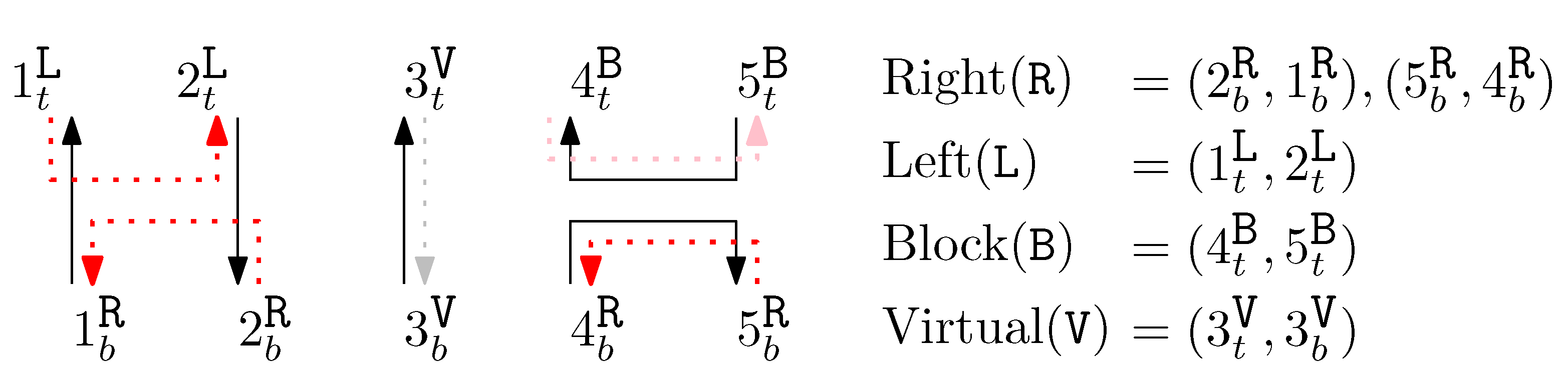
• Side-aware DNA origami words, consisting of scaffolds and staples, are represented by graphical structures of width n. These graphical structures contain n columns, and each column has two endpoints: top and bottom. Scaffolds and staples are represented by directed pairs of endpoints. By combining the set of pairs of scaffolds and the set of pairs of staples, we define a graphical structure. Details are described in Section 3.1.
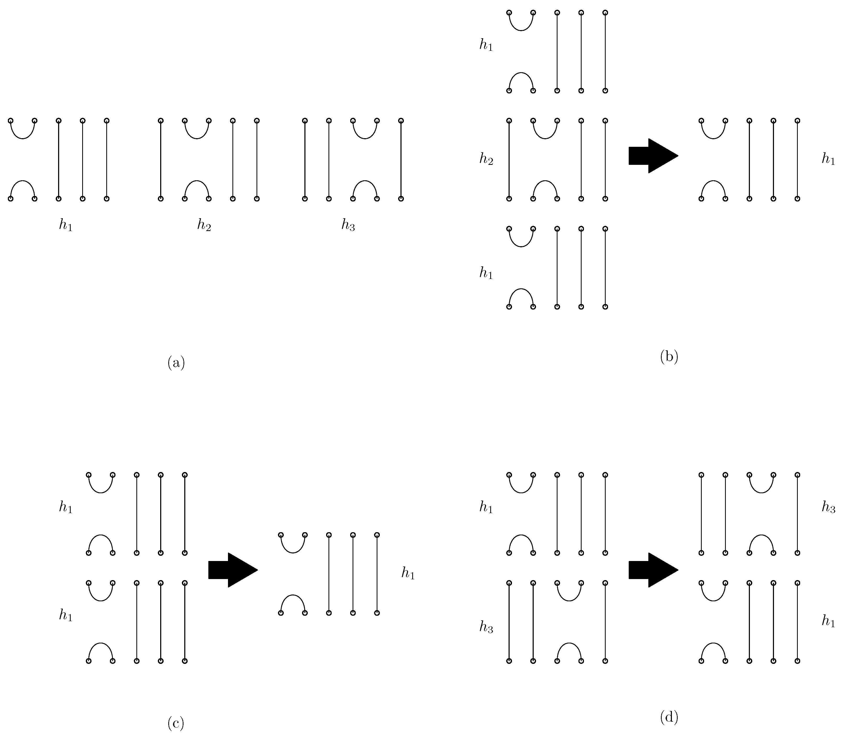
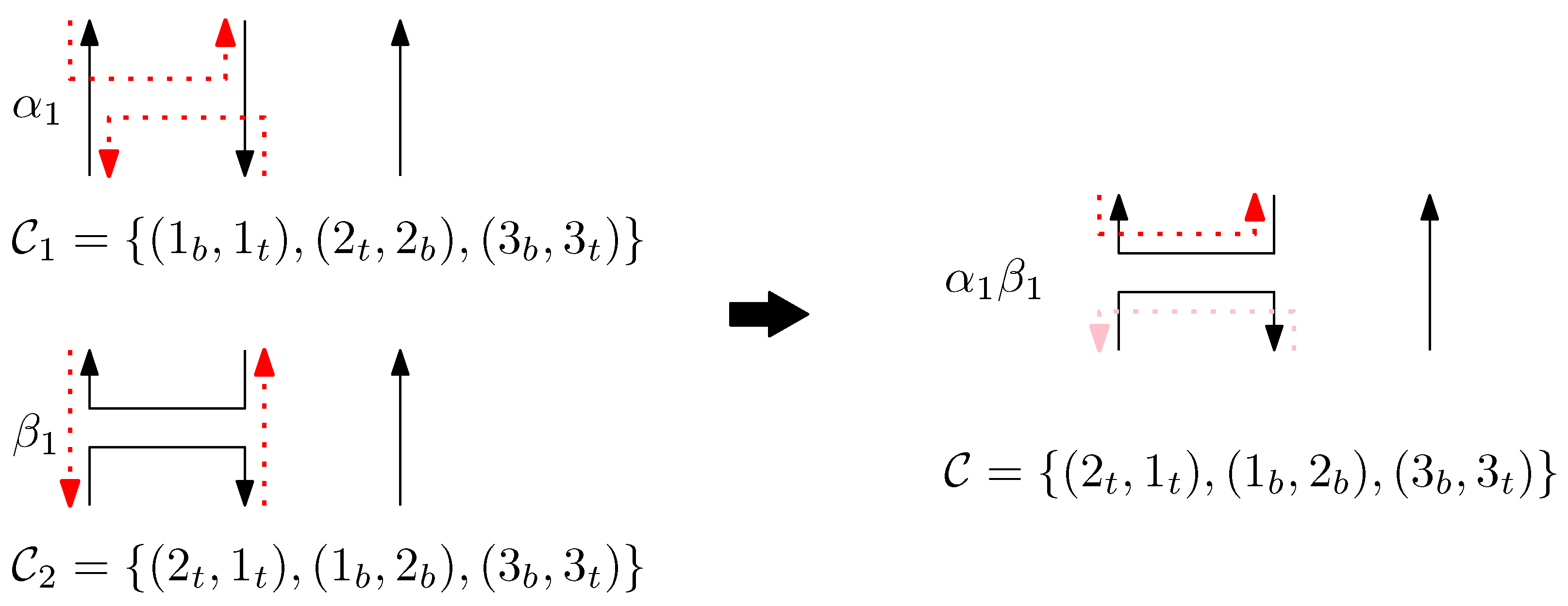
• We define the concatenation of two graphical structures of side-aware DNA origami words. This concatenation is based on the relations of the Jones monoid and its graphical representation, as described in Figure 1. Unlike the classical concatenation of words, the concatenation of graphical structures is performed vertically, aligning their columns. Details are described in Section 3.2.

3.1. Side-Aware DNA Origami Words

We define columns consisting of scaffolds and staples, where the staples align along the scaffolds with the following properties:

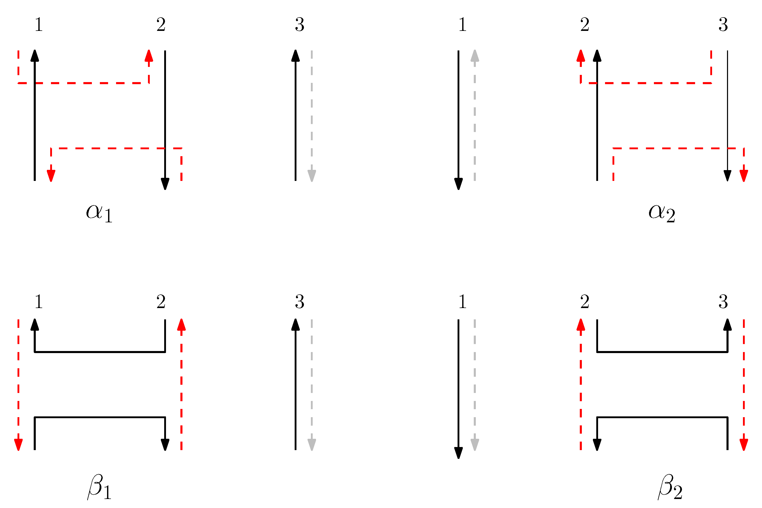
• We observe that there are two different types of motifs in the DNA origami structure: there are places where two adjacent scaffolds connect the two columns, and also places where two adjacent staples connect the two columns.
• The scaffolds and staples have directions: adjacent scaffolds are anti-parallel, and a staple is anti-parallel to the connected scaffold.
• Each staple end can reside on two different sides of the connected scaffold—left and right.

To represent such scaffolds and staples by directed pairs of endpoints, we first define the set of geometric positions to represent locations of points. Given n as the width of the graphical structure, we first define $x=i_t$ (respectively, $i_b$) to represent a position at the top (respectively, bottom) of the ith column for $1\le i\le n$. We assume that scaffolds at the ith column go upward if i is odd, and downward if i is even, and the direction of the staples is opposite from the direction of the scaffolds. The set of geometric positions for given n is defined as $E_n=\{i_t,i_b\mid 1\le i\le n\}$.

A scaffold segment is defined by an ordered pair $(x,y)$ of endpoints where $x,y\in E_n$. For a staple segment, each segment is categorized into four different types:

• Virtual (V): A staple is not present on the given column (we formally regard this “absence” of a staple as one type of staple for the concise definition of concatenation of structures). Other staples can be extended on a virtual staple through concatenation.
• Left (L): Two endpoints of the staple are on the left side of the scaffolds.
• Right (R): Two endpoints of the staple are on the right side of the scaffolds.
• Block (B): A staple is disconnected in-between. Other staples cannot be extended on a block staple through concatenation.

Thus, a staple segment is defined by an ordered pair $(x^{\mathtt{d}},y^{\mathtt{d}})$ of endpoints where $x,y\in E_n$ and $\mathtt{d}\in \{\mathtt{V},\mathtt{B},\mathtt{L},\mathtt{R}\}$. Figure 2 shows an example of staple segments over $E_5$. Then, a graphical structure is defined as a pair $(\mathcal{C},\mathcal{P})$ of a set of scaffold segments and a set of staple segments that satisfies the following condition: each position in $E_n$ is occupied exactly once by endpoints in $\mathcal{C}$ ($\mathcal{P}$). For any segment $s=(x,y)$ of endpoints, we define the reverse of the segment as $\overleftarrow{s}=(y,x)$, which is defined similarly to a set of segments.

For a given width n, we define basic modules and corresponding generators ${\Sigma }_n=\{{\alpha }_i,{\beta }_i\mid 1\le i\le n-1\}$ as an alphabet for DNA origami words with the order ${\alpha }_1<\cdots <{\alpha }_{n-1}<{\beta }_1<\cdots <{\beta }_{n-1}$. We say that ${\alpha }_i$ is complementary to ${\beta }_i$, and vice versa. For each generator ${\alpha }_i$ and ${\beta }_i$ we have four maps as described below:

• ${\alpha }_i=\{(i_b,i_t),({\left(i+1\right)}_t,{\left(i+1\right)}_b),(i_t^{\mathtt{L}},{(i+1)}_t^{\mathtt{L}}),({(i+1)}_b^{\mathtt{R}},i_b^{\mathtt{R}})\}$
• ${\beta }_i=\{({(i+1)}_t,i_t),(i_b,{(i+1)}_b),(i_t^{\mathtt{L}},i_b^{\mathtt{L}}),({(i+1)}_b^{\mathtt{R}},{(i+1)}_b^{\mathtt{R}})\}$

We call four maps that describe ${\alpha }_i$ (respectively, ${\beta }_i$) units for ${\alpha }_i$ (respectively, ${\beta }_i$). Note that units are reversed for even is. The units for each generator describe their structures between the ith and the $(i+1)$st columns.

Table 1. Units for generators of odd is (pairs are reversed for even is).

	${\mathcal{R}}_{\mathit{c}}$	${\mathcal{R}}_{\mathit{p}}$
${\alpha }_i$	$(i_b,i_t),({i+1}_t,{i+1}_b)$	$(i_t^{\mathtt{L}},{i+1}_t^{\mathtt{L}}),({i+1}_b^{\mathtt{R}},i_b^{\mathtt{R}})$
${\beta }_i$	$({i+1}_t,i_t),(i_b,{i+1}_b)$	$(i_t^{\mathtt{L}},i_b^{\mathtt{L}}),({i+1}_b^{\mathtt{R}},{i+1}_t^{\mathtt{R}})$

shows the units for generators of odd is.

The full graphical structure $G\left({\gamma }_i\right)$ for ${\gamma }_i$ must include not only the units for the ith and $(i+1)$st columns but also the remaining columns to fully represent a complete structure of size n. The structure of each generator ${\gamma }_i\in {\Sigma }_n$ has a context $\mathcal{T}\left({\gamma }_i\right)$ which consists of a scaffold $(k_b,k_t)$ and a staple $(k_t^{\mathtt{V}},k_b^{\mathtt{V}})$ for odd ks and their reverses for even ks where $k\notin \{i,i+1\}$. Figure 3 illustrates the graphical structure of ${\alpha }_i,{\alpha }_{i+1},{\beta }_i$, and ${\beta }_{i+1}$ of size 3, including the context corresponding to the 3rd column, with $i=1$. We notice that context $\mathcal{T}\left({\gamma }_i\right)$ can have real or virtual pairs of scaffolds and staples. Based on the choice of r, we observe that the context $\mathcal{T}\left({\gamma }_i\right)$ can include either real or virtual pairs of scaffolds and staples. Depending on the choice of real or virtual context, different structural descriptions of graphical structures are possible [5]:

• ${\mathcal{G}}_{max\left(n\right)}$: The entire context is real, with both ${\mathcal{V}}_c$ and ${\mathcal{V}}_p$ being empty.
• ${\mathcal{G}}_{mid\left(n\right)}$: The context for the scaffold is real, while the context for the staple is virtual.
• ${\mathcal{G}}_{min\left(n\right)}$: The entire context is virtual.

In this study, we focus on ${\mathcal{G}}_{max\left(n\right)}$, as the four types of staples enhance the structural diversity.

Figure 3. Graphical structure of ${\alpha }_i$s and ${\alpha }_{i+1}$, where $i=1$. Real scaffolds are represented by black lines and real staples are represented by red dashed lines. Virtual staples are grey dashed lines. Virtual staples can be assigned to either the left or right side of a scaffold, but in this figure, we assign the virtual staples to the right side of a scaffold. In the graphical structure of ${\alpha }_1$, the context ${\mathcal{T}}_1$ contains $(3_b,3_t)\in {\mathcal{R}}_c$ and $(3_b^{ϵ},3_t^{ϵ})\in {\mathcal{V}}_p$. The pair $(3_b^{ϵ},3_t^{ϵ})$ shows that the virtual staple has possible strands to either the left or right of the scaffold $(3_t,3_t)$.

Figure 3. Graphical structure of ${\alpha }_i$s and ${\alpha }_{i+1}$, where $i=1$. Real scaffolds are represented by black lines and real staples are represented by red dashed lines. Virtual staples are grey dashed lines. Virtual staples can be assigned to either the left or right side of a scaffold, but in this figure, we assign the virtual staples to the right side of a scaffold. In the graphical structure of ${\alpha }_1$, the context ${\mathcal{T}}_1$ contains $(3_b,3_t)\in {\mathcal{R}}_c$ and $(3_b^{ϵ},3_t^{ϵ})\in {\mathcal{V}}_p$. The pair $(3_b^{ϵ},3_t^{ϵ})$ shows that the virtual staple has possible strands to either the left or right of the scaffold $(3_t,3_t)$.

3.2. Concatenation of Side-Aware DNA Origami Words

We now introduce how side-aware DNA origami structures are concatenated based on the relations of Jones monoid and its graphical representation. The graphical structure corresponding to the concatenation of two words is formed by placing the graphical structure of the first word on top of that of the second word. When a virtual staple meets a left (or right) staple, the virtual staple becomes the left (or right) staple. This process demonstrates that the empty space represented by a virtual staple can be extended through concatenation, depending on whether it encounters a left or right staple. In contrast, if a left (or right) staple meets a right (or left) staple, both staples become blocked, meaning the staples are disconnected.

For two graphical structures of words $w_1$ and $w_2$, the concatenation $w_1·w_2=w$ is defined as follows: suppose $G\left(w_1\right)=({\mathcal{C}}_1,{\mathcal{P}}_1)$ and $G\left(w_2\right)=({\mathcal{C}}_2,{\mathcal{P}}_2)$ are graphical structures of $w_1$ and $w_2$, respectively. We now describe the procedure to define the graphical structure $G\left(w\right)$, the concatenation of the two words $w_1$ and $w_2$, with the set $\mathcal{C}$ of scaffolds and the set $\mathcal{P}$ of staples. Note that $G\left(w\right)=G\left(w_1{w}_2\right)=(\mathcal{C},\mathcal{P})$.

First, the set $\mathcal{C}$ of scaffolds is obtained as follows:

(i)

For all scaffolds in ${\mathcal{C}}_1$, replace the subscript b by m.

(ii)

For all scaffolds in ${\mathcal{C}}_2$, replace the subscript t by m.

(iii)

Given set ${\mathcal{C}}_1\cup {\mathcal{C}}_2$, for each sequence

$$\left(q\right(0),q(1\left)\right),\left(q\right(1),q(2\left)\right),\dots ,\left(q\right(v-1),q(v\left)\right)$$

of scaffolds where points $q\left(0\right)$ and $q\left(v\right)$ have subscripts t or b, add $\left(q\right(0),q(v\left)\right)$ to $\mathcal{C}$. Figure 4 shows an example of the set $\mathcal{C}$ of scaffolds of a graphical structure $G\left(w\right)=(\mathcal{C},\mathcal{P})$ of a word $w={\alpha }_1{\beta }_1$.

Set $\mathcal{P}$ of staples is obtained as follows:

(i)

For all staples in ${\mathcal{P}}_1$, replace the subscript b by m.

(ii)

For all staples in ${\mathcal{P}}_2$, replace the subscript t by m.

(iii)

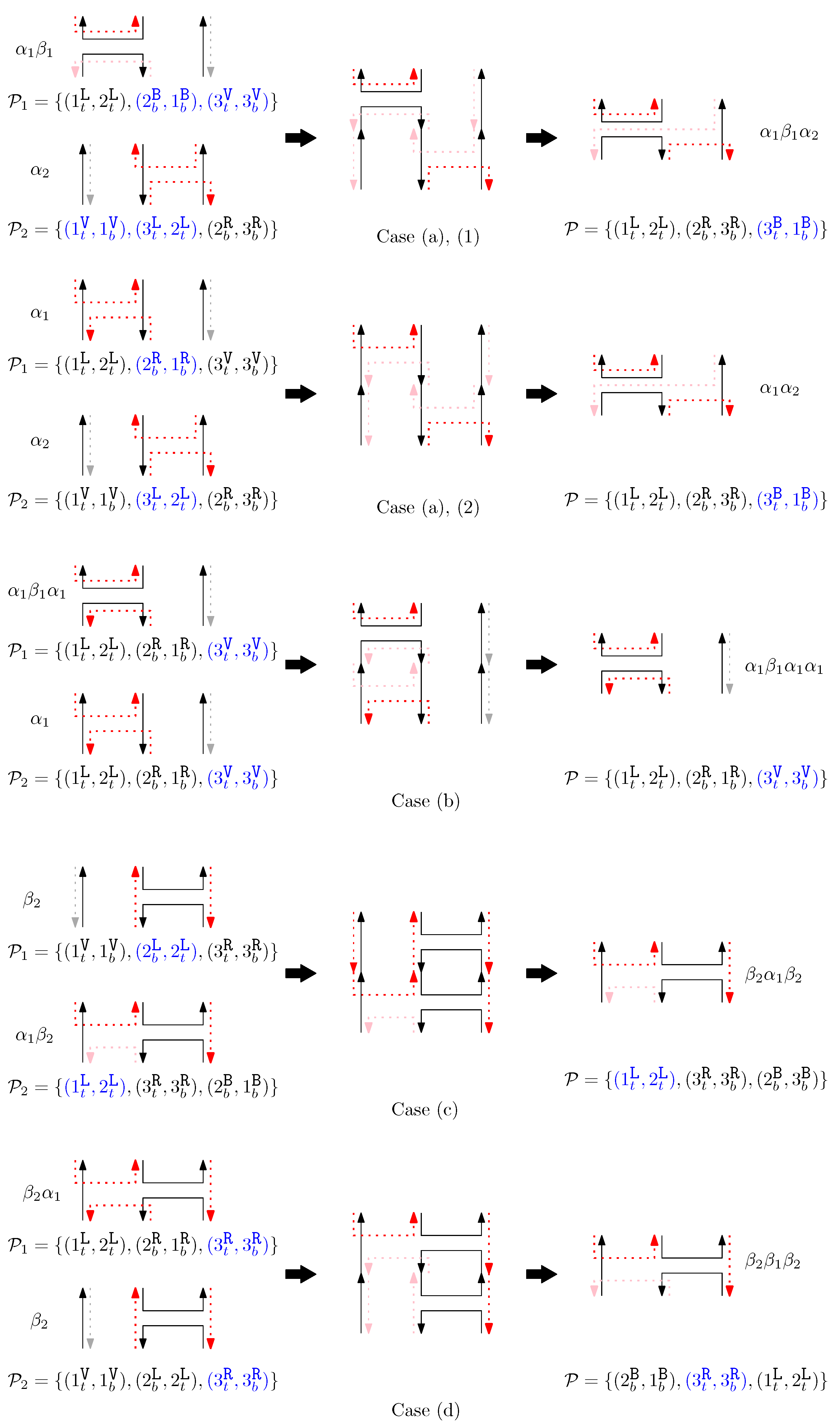
Given set ${\mathcal{P}}_1\cup {\mathcal{P}}_2$, for each sequence

$$(q{\left(0\right)}^{d\left(0\right)},q{\left(1\right)}^{d\left(0\right)}),(q{\left(1\right)}^{d\left(1\right)},q{\left(2\right)}^{d\left(1\right)}),\dots ,(q{(v-1)}^{d(v-1)},q{\left(v\right)}^{d(v-1)})$$

of staples where $q\left(i\right)$s denote positions, $d\left(i\right)$s denote staple types and points $q{\left(0\right)}^{d\left(0\right)}$, and $q{\left(v\right)}^{d(v-1)}$ have subscripts t or b, we perform the following:

(a)

If (1) $d\left(i\right)=\mathtt{B}$ or (2) $d\left(i\right)=\mathtt{L}$ and $d(i+1)=\mathtt{R}$ or (3) $d\left(i\right)=\mathtt{R}$ and $d(i+1)=\mathtt{L}$ for any $0\le i\le v-1$, add $(q{\left(0\right)}^{\mathtt{B}},q{\left(v\right)}^{\mathtt{B}})$ to $\mathcal{P}$.

(b)

Otherwise, if $d\left(i\right)=\mathtt{V}$ for all $0\le i\le v-1$, add $(q{\left(0\right)}^{\mathtt{V}},q{\left(v\right)}^{\mathtt{V}})$ to $\mathcal{P}$.

(c)

Otherwise, if $d\left(i\right)=\mathtt{L}$ for any $0\le i\le v-1$, add $(q{\left(0\right)}^{\mathtt{L}},q{\left(v\right)}^{\mathtt{L}})$ to $\mathcal{P}$.

(d)

Otherwise, add $(q{\left(0\right)}^{\mathtt{R}},q{\left(v\right)}^{\mathtt{R}})$ to $\mathcal{P}$.

Figure 5 shows an example of each case (a)–(d).

We observe that the composition of graphical structures is associative, that is, $G\left(w_1{w}_2{w}_3\right)=G\left(\left(w_1{w}_2\right)w_3\right)=G\left(w_1\left(w_2{w}_3\right)\right)$. We use ${\mathcal{G}}_e\left(n\right)$ to refer to the set of all graphical structures that can be constructed from ${\Sigma }_n$.

4. Side-Aware DNA Origami Rewriting Systems

In this section, we introduce rewriting rules for two graphical structures corresponding to $w_1$ and $w_2$. Specifically, if two words $w_1$ and $w_2$ produce the same graphical structure, i.e., $G\left(w_1\right)=G\left(w_2\right)$, then $w_1$ can be rewritten as $w_2$, and vice versa. Since the concatenation of two graphical structures occurs in a horizontal manner, the types of endpoints at the bonding sites influence the resulting structure. For instance, the bottom endpoints of the graphical structure of $G\left(w_1\right)$ and the top endpoints of the graphical structure of $G\left(w_2\right)$ determine the outcome of the concatenated structure $G(w_1·w_2)$. If the bottom endpoints of $G\left(w_1\right)$ have a “cap” shape, with two endpoints connected from the bottom of one column to the bottom of the adjacent column, how does this affect the resulting structures when considering all possible generators that could bond below $G\left(w_1\right)$? Note that it is worth noting that a “cup” shape at the bottom endpoints of $G\left(w_1\right)$ does not constrain or affect other generators bonding below $G\left(w_1\right)$, as it does not interfere with the bonding process. Conversely, if the top endpoints of $G\left(w_2\right)$ have a “cup” shape, with two endpoints connected from the top of one column to the top of the adjacent column, how does this influence the resulting structures when considering all possible generators that could bond above $G\left(w_2\right)$?

We define the rewriting rules as patterns of structural types and describe how each structural type affects the resulting structures. The concept of side-aware DNA origami words, which allows for the directional binding of staples to the scaffold, increases the complexity of the rewriting rules, even with only six possible generators to concatenate. We note that if the gap between columns is greater than two, the resulting structures are unaffected by the relations in the Jones monoid. Therefore, we only need to consider six generators: ${\alpha }_{i-2},{\alpha }_{i-1},{\alpha }_i,{\beta }_{i-2},{\beta }_{i-1},{\beta }_i$.

4.1. Rewriting Rules

We define a rewriting rule $w_1\leftrightarrow w_2$ under ${\mathcal{G}}_e\left(n\right)$ if $G\left(w_1\right)=G\left(w_2\right)$ under ${\mathcal{G}}_e\left(n\right)$. Here, we establish the finite set of rewriting rules $R_e\left(n\right)$ under ${\mathcal{G}}_e\left(n\right)$. For convenience, we use $\gamma$ and $\delta$ to represent an arbitrary generator type ($\alpha$ or $\beta$), and $\overline{\gamma }$ to represent a complementary generator of $\gamma$. We observe the following statements:

• If $w_1\leftrightarrow w_2$ under ${\mathcal{G}}_e\left(n\right)$, then $w_1\leftrightarrow w_2$ under ${\mathcal{G}}_{max}\left(n\right)$. Namely, if two graphical structures $G\left(w_1\right)$ and $G\left(w_2\right)$ are the same under ${\mathcal{G}}_e\left(n\right)$, then they should be the same when we ignore sides of staples and connect all staple endpoints at the same position. This implies that for any rule $w_1\leftrightarrow w_2\in R_e\left(n\right)$, there exist $w_1^{\prime }\leftrightarrow w_2^{\prime }\in R_{max}\left(n\right)$, and words $w_{⊏}^{\prime }$ and $w_{⊐}^{\prime }$ such that $w_1=w_{⊏}^{\prime }{w}_1^{\prime }{w}_{⊐}^{\prime }$ and $w_2=w_{⊏}^{\prime }{w}_2^{\prime }{w}_{⊐}^{\prime }$.
• If $w_1\leftrightarrow w_2$ under ${\mathcal{G}}_{max}\left(n\right)$, then the scaffolds of $G\left(w_1\right)$ and $G\left(w_2\right)$ are the same under ${\mathcal{G}}_e\left(n\right)$.
• Staple segments in the generators are categorized into three geometric types: a cap (i.e., $(1_b^{\mathtt{R}},2_b^{\mathtt{R}})$), a cup (i.e., $(2_t^{\mathtt{R}},1_t^{\mathtt{R}})$), and a straight segment (i.e., ($(3_b^{\mathtt{B}},3_t^{\mathtt{B}})$)). For convenience, we refer to a cap (cup) between the ith and the $i-1$st columns as the ith cap (cup), and a straight staple at the ith column as the ith straight staple.

Under these observations, for each pair $\left(s\right(i),r(i\left)\right)$ of staple segments with the same start and end positions dependent on i, we establish a set $\left\{(w_{⊏},w_{⊐})\right\}$ of pairs of a prefix $w_{⊏}\in {\Sigma }^{*}$ and a suffix $w_{⊐}\in {\Sigma }^{*}$ that satisfies the following condition: for any pair $(w_1,w_2)$ of words where $G\left(w_1\right)$ and $G\left(w_2\right)$ are the same under ${\mathcal{G}}_e\left(n\right)$ except $s\left(i\right)$ in $G\left(w_1\right)$ and $r\left(i\right)$ in $G\left(w_2\right)$, the equality $G\left(w_{⊏}{w}_1{w}_{⊐}\right)=G\left(w_{⊏}{w}_2{w}_{⊐}\right)$ holds under ${\mathcal{G}}_e\left(n\right)$. We call such set an override set, denoted by $O_C\left(i\right)$, where $C\in \{cap,cup,\mathtt{R}\mathtt{B},\mathtt{L}\mathtt{B},\mathtt{V}\mathtt{R},\mathtt{V}\mathtt{L},\mathtt{V}\mathtt{B}\}$ represents the type of the pairs. Then, for each rule $w_1^{\prime }\leftrightarrow w_2^{\prime }\in R_{max}\left(n\right)$, we observe the staple difference between $G\left(w_1^{\prime }\right)$ and $G\left(w_2^{\prime }\right)$ under ${\mathcal{G}}_e\left(n\right)$, concatenate a prefix and a suffix from the corresponding override set to make the graphical structures equivalent, and retrieve the rewriting rules under ${\mathcal{G}}_e\left(n\right)$.

An override set is a collection of “prefix–suffix pairs” that can adjust two words to make their graphical structures equivalent, even if there is a specific difference between them in terms of staple segments. For any given type of difference—like a “cap” or “cup” at a certain position—this set provides the necessary adjustments to “override” that difference. If two DNA origami words would result in the same structure except for a small discrepancy in their staples at position i, the override set tells us how to add the same prefix and suffix around both words so that their final structures become identical.

Below is the list of each pair of staple segments and the corresponding override sets.

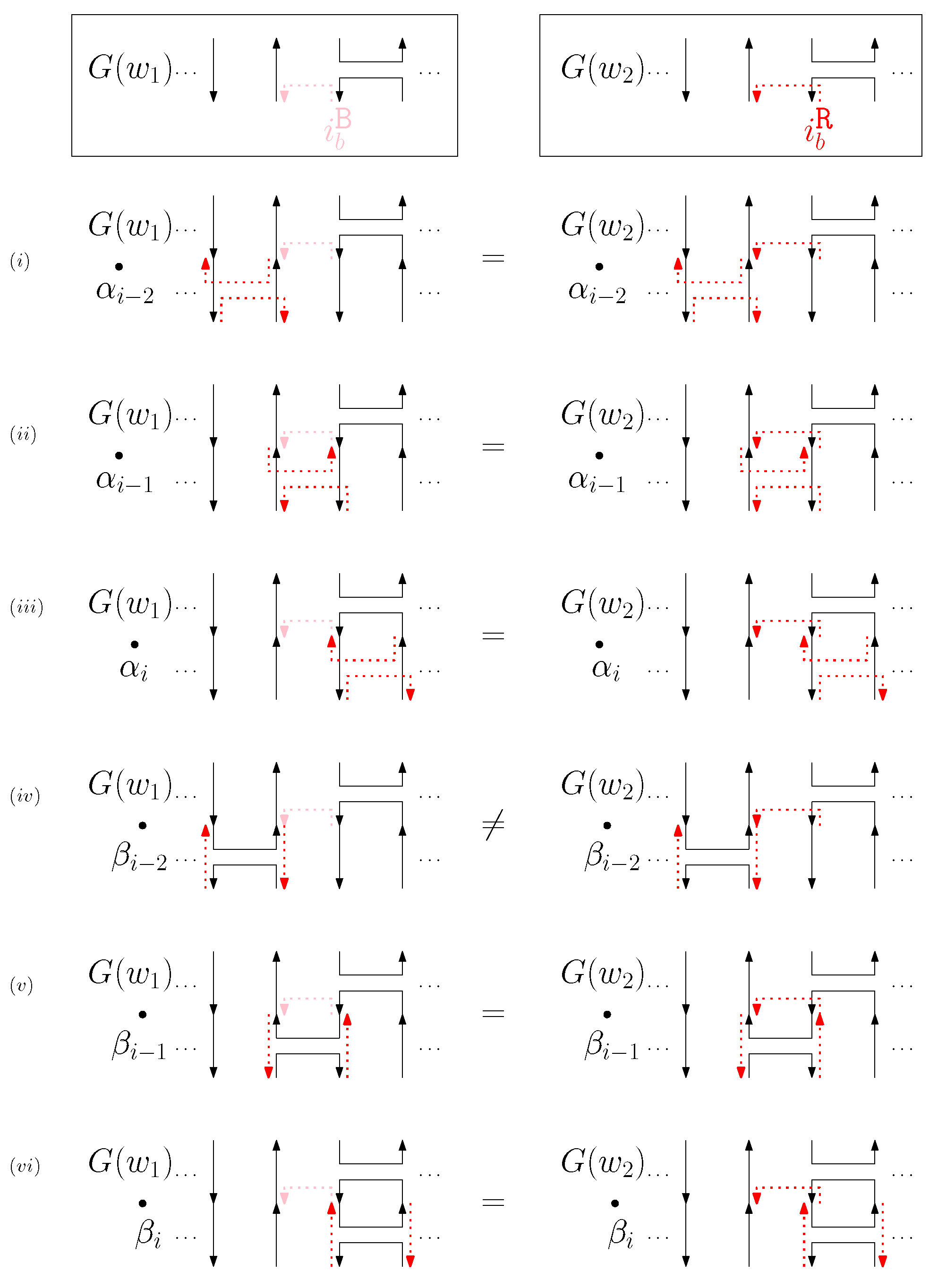
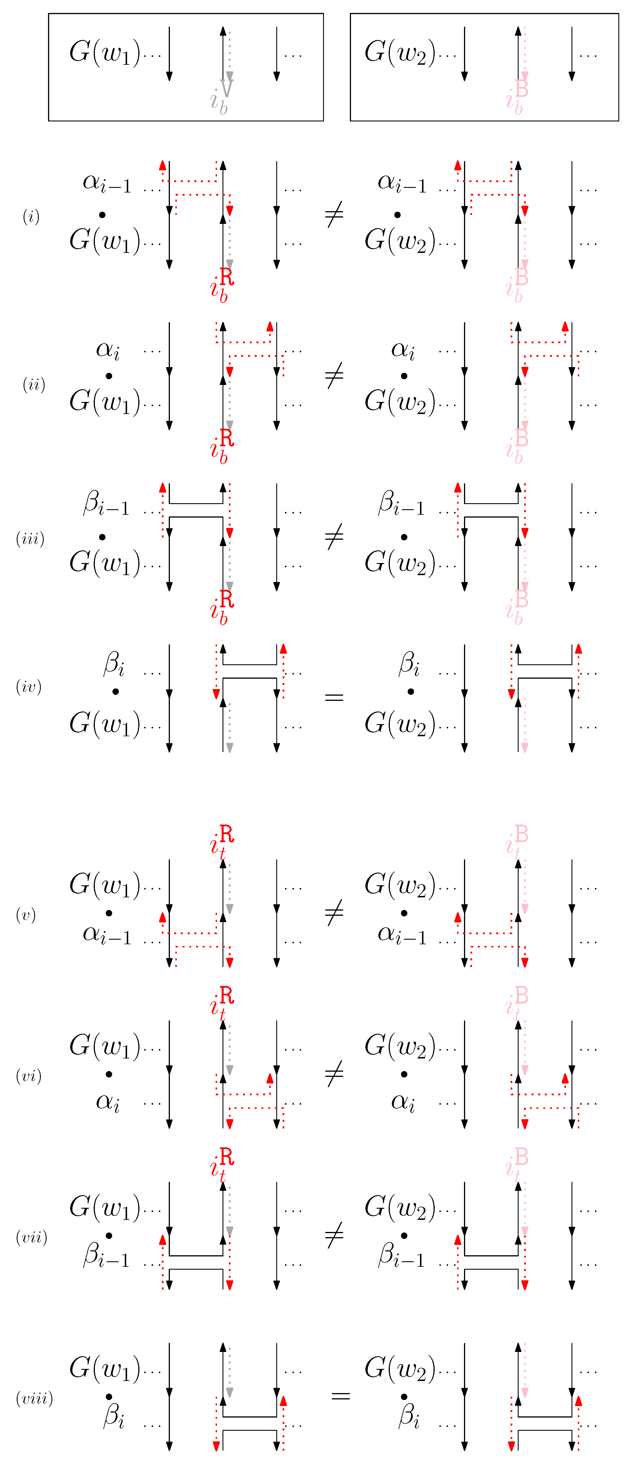
• Cap: We first consider a pair $\left(s\left(i\right)=(i_b^{\mathtt{B}},{(i-1)}_b^{\mathtt{B}}),r\left(i\right)=(i_b^{\mathtt{R}},{(i-1)}_b^{\mathtt{R}})\right)$ of ith caps for even is. Since the cap segments are at the bottom of the structure, concatenating any prefix does not affect the equivalence of graphical structures. We have six different generators that affect the ith cap segments: ${\gamma }_{i-2}$ through ${\gamma }_i$. Figure 6 illustrates an example of $G\left(w_1\right)$ and $G\left(w_2\right)$ where the only difference is $\left(s\right(i),r(i\left)\right)$, and changes in the graphical structures from concatenation of these six generators after $w_1$ and $w_2$. We observe that all generators except ${\beta }_{i-2}$ make two graphical structures equivalent. For the ${\beta }_{i-2}$ case, the difference in graphical structures remains the same. Therefore, we establish the override set as $O_{cap}\left(i\right)=\left\{(ϵ,vz)\mid v\in {({\Sigma }_n\setminus Z)}^{*},z\in Z\right\}$ for $Z=\{{\alpha }_{i-2},{\alpha }_{i-1},{\alpha }_i,{\beta }_{i-1},{\beta }_i\}$. When i is odd, for $\left(\overleftarrow{s\left(i\right)},\overleftarrow{r\left(i\right)}\right)$, the override set is the same as the even case, which holds for all of the following cases.
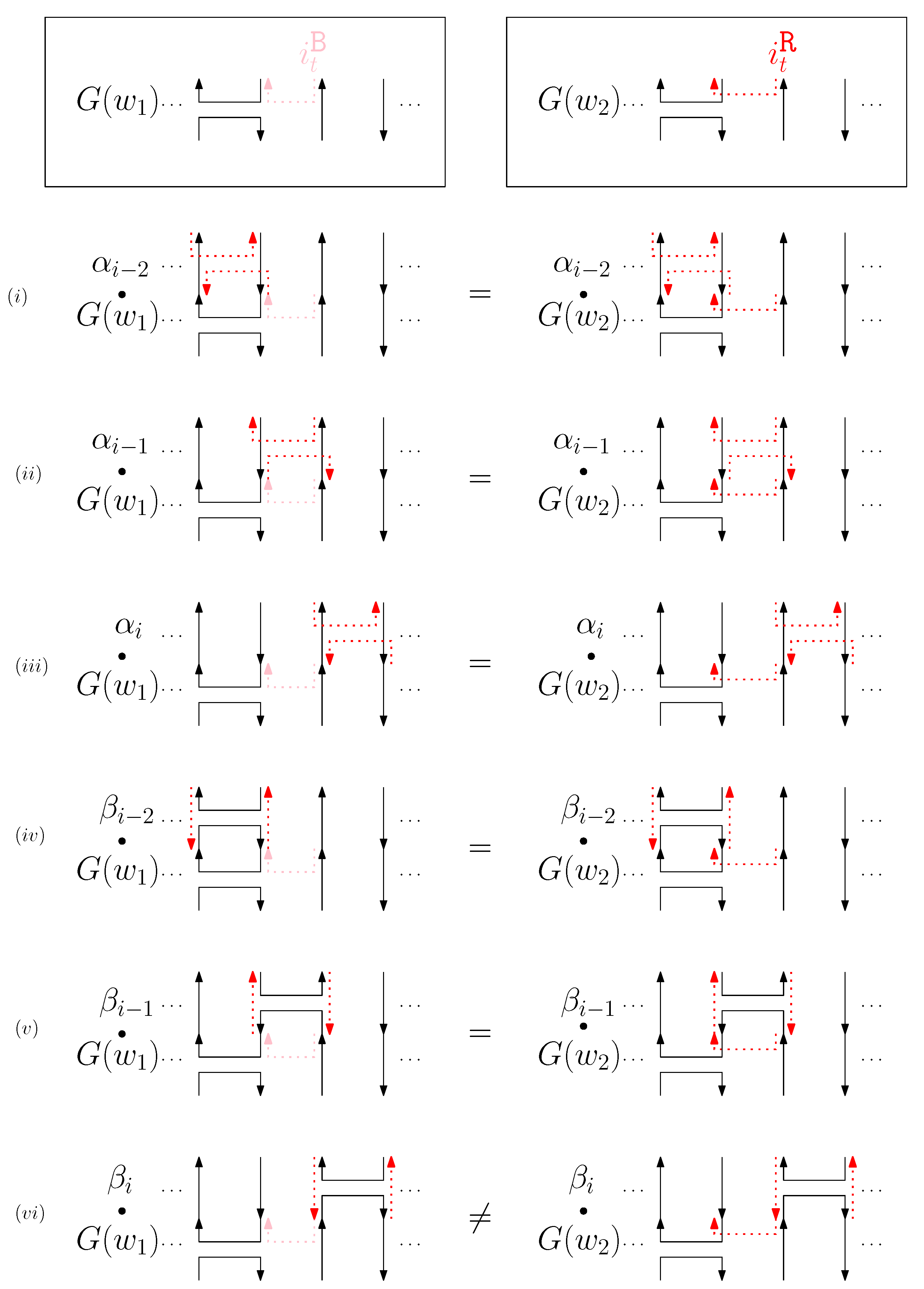
• Cup: We consider a pair $\left(s\left(i\right)=(i_t^{\mathtt{B}},{(i-1)}_t^{\mathtt{B}}),r\left(i\right)=(i_t^{\mathtt{L}},{(i-1)}_t^{\mathtt{L}})\right)$ of ith cups for odd is. Since the cup segments are at the top of the structure, concatenating any suffix does not affect the equivalence of graphical structures. We have six different generators that affect the ith cap segments: ${\gamma }_{i-2}$ through ${\gamma }_i$. Figure 7 illustrates an example of $G\left(w_1\right)$ and $G\left(w_2\right)$ where the only difference is $\left(s\right(i),r(i\left)\right)$, and changes in the graphical structures from concatenation of these six generators before $w_1$ and $w_2$. We observe that all generators except ${\beta }_i$ make two graphical structures equivalent. For the ${\beta }_i$ case, the difference in graphical structures remains the same. Therefore, we establish the override set as $O_{cup}\left(i\right)=\left\{(zv,ϵ)\mid v\in {({\Sigma }_n\setminus Z)}^{*},z\in Z\right\}$ for $Z=\{{\alpha }_{i-2},{\alpha }_{i-1},{\alpha }_i,{\beta }_{i-2},{\beta }_{i-1}\}$.
• Straight segment: We have the following cases.

  (a)

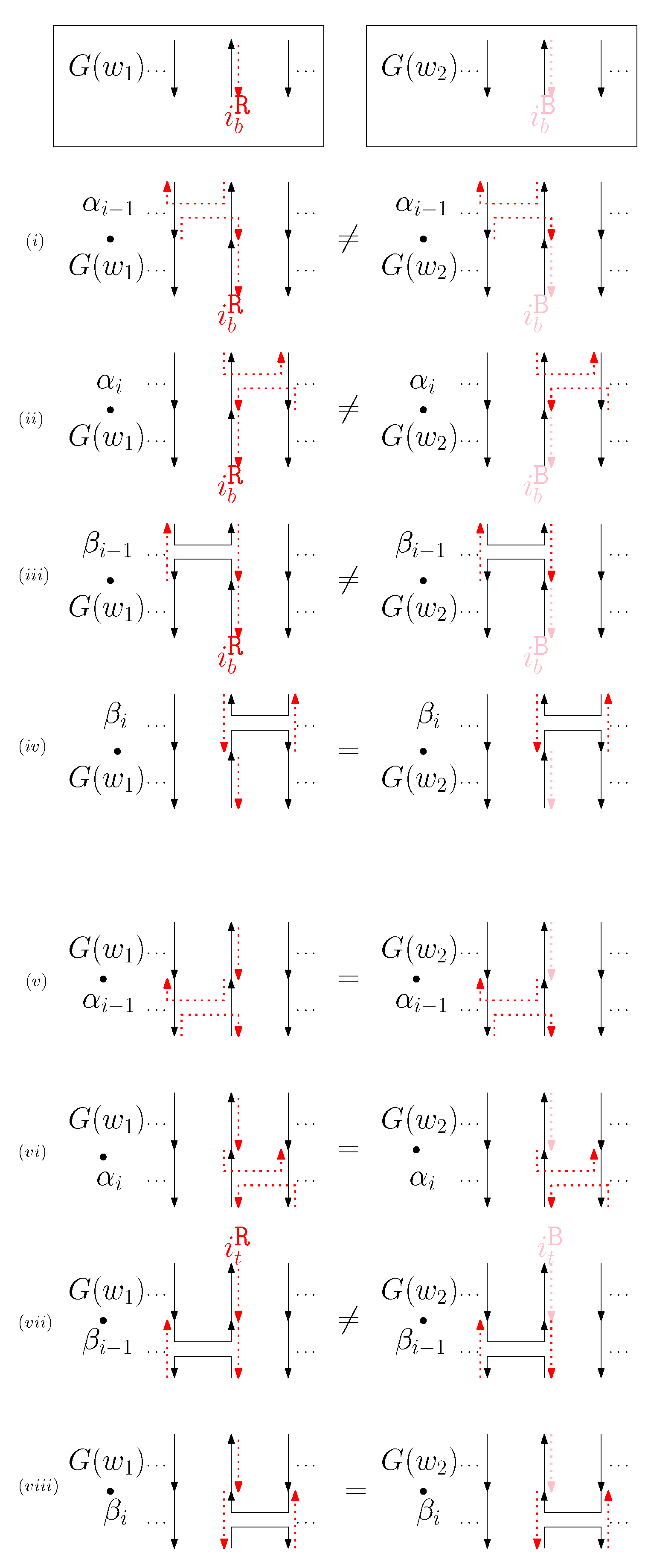
  When $s\left(i\right)$ is right and $r\left(i\right)$ is block: we consider $\left(s\left(i\right)=(i_t^{\mathtt{R}},i_b^{\mathtt{R}}),r\left(i\right)=(i_t^{\mathtt{B}},i_b^{\mathtt{B}})\right)$ for odd is. We have four different generators that affect the straight segments: ${\gamma }_{i-1}$ through ${\gamma }_i$. Figure 8 illustrates an example of $G\left(w_1\right)$ and $G\left(w_2\right)$ where the only difference is $\left(s\right(i),r(i\left)\right)$, and changes in the graphical structures from concatenation of these four generators before and after $w_1$ and $w_2$. If concatenation of a generator does not make two graphical structures equivalent, it may change the geometric type of the staple segment difference. For example, concatenating ${\alpha }_i$ before $w_1$ and $w_2$ changes the geometric type of the staple segment difference to the $i+1$st cap. Thus, for any $(ϵ,w_{⊐}^{\prime })\in O_{cap}(i+1)$, $G\left({\alpha }_i{w}_1{w}_{⊐}^{\prime }\right)=G\left({\alpha }_i{w}_2{w}_{⊐}^{\prime }\right)$ holds. We summarize all of the cases as the following override set: $O_{\mathtt{R}\mathtt{B}}\left(i\right)=\left\{({\beta }_{i}v,ϵ)\right\}\cup \left\{(ϵ,vz)\mid z\in Z\right\}\cup \left\{({\alpha }_{i-1}v,w_{⊐}^{\prime })\mid (ϵ,w_{⊐}^{\prime })\in O_{cap}\left(i\right)\right\}$ $\cup \left\{({\alpha }_{i}v,w_{⊐}^{\prime })\mid (ϵ,w_{⊐}^{\prime })\in O_{cap}(i+1)\right\}$ for $Z=\{{\alpha }_{i-1},{\alpha }_i,{\beta }_i\}$ and $v\in {({\Sigma }_n\setminus Z)}^{*}$.

  (b)

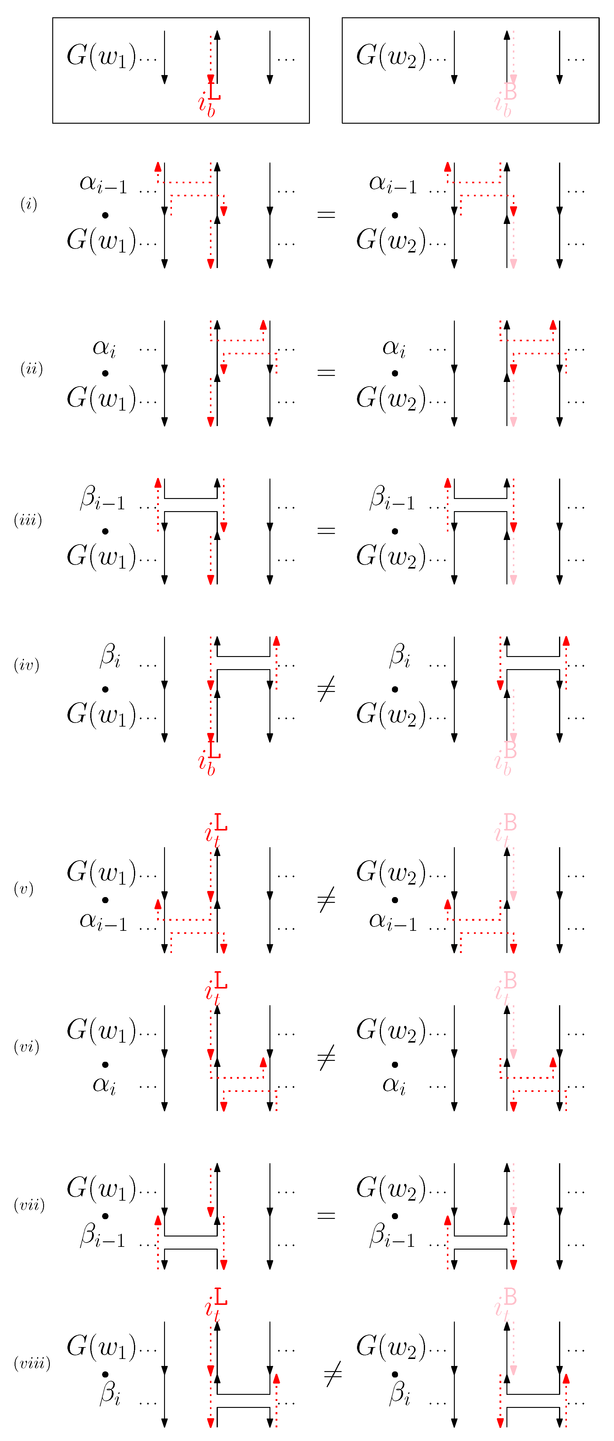
  When $s\left(i\right)$ is left and $r\left(i\right)$ is block: we consider $\left(s\left(i\right)=(i_t^{\mathtt{L}},i_b^{\mathtt{L}}),r\left(i\right)=(i_t^{\mathtt{B}},i_b^{\mathtt{B}})\right)$ for odd is in Figure 9. We establish the following override set: $O_{\mathtt{L}\mathtt{B}}\left(i\right)=\left\{(zv,ϵ)\mid z\in Z\right\}\cup \left\{(ϵ,v{\beta }_{i-1})\right\}\cup \left\{(w_{⊏}^{\prime },v{\alpha }_{i-1})\mid (w_{⊏}^{\prime },ϵ)\in O_{cup}\left(i\right)\right\}$ $\cup \left\{(w_{⊏}^{\prime },v{\alpha }_i)\mid (w_{⊏}^{\prime },ϵ)\in O_{cup}(i+1)\right\}$ for $Z=\{{\alpha }_{i-1},{\alpha }_i,{\beta }_{i-1}\}$ and $v\in {({\Sigma }_n\setminus Z)}^{*}$.

  (c)

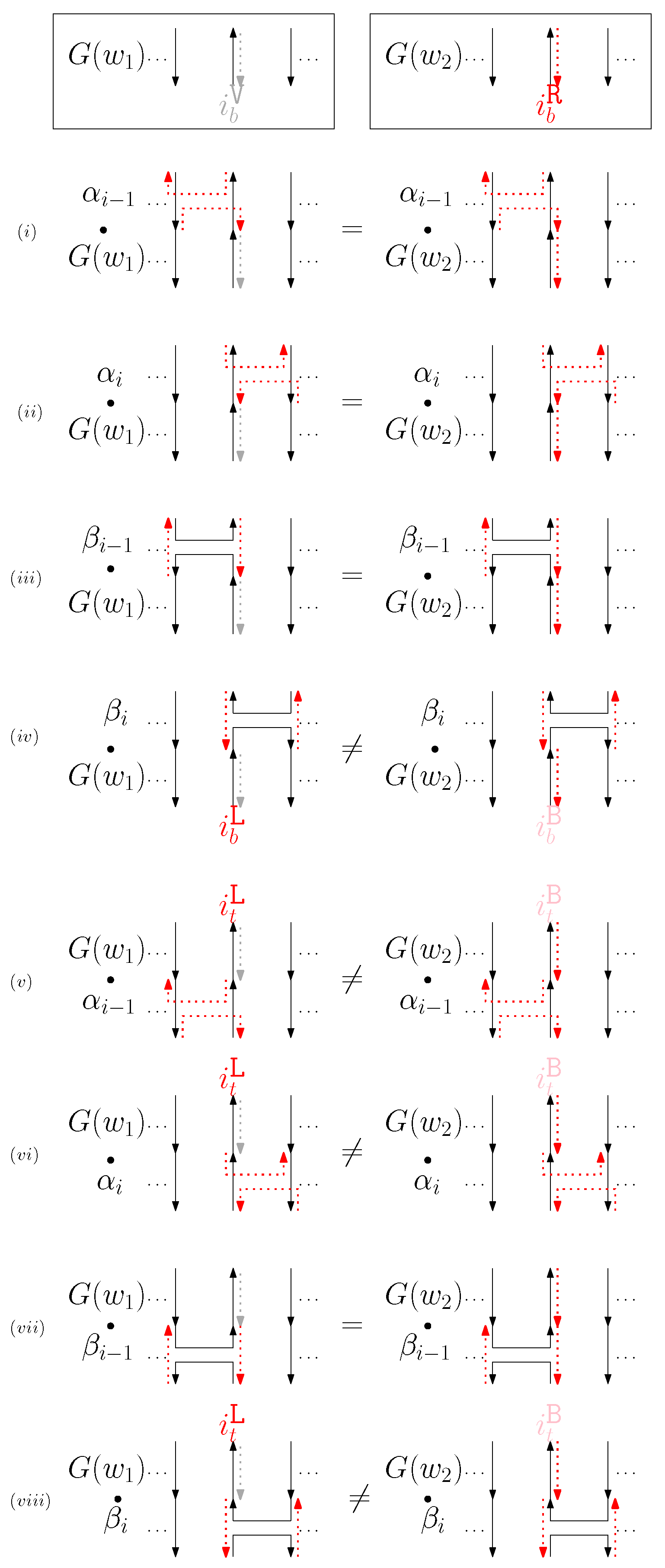
  When $S\left(i\right)$ is virtual and $r\left(i\right)$ is right: We first consider $\left(s\left(i\right)=(i_t^{\mathtt{V}},i_b^{\mathtt{V}}),r\left(i\right)=(i_t^{\mathtt{R}},i_b^{\mathtt{R}})\right)$ for odd is in Figure 10. We summarize all of the cases as the following override set: $O_{\mathtt{V}\mathtt{R}}\left(i\right)=\left\{(zv,ϵ)\mid z\in \{{\alpha }_{i-1},{\alpha }_i,{\beta }_{i-1}\}\right\}\cup \left\{(ϵ,v{\beta }_{i-1})\right\}\cup$ $\left\{(w_{⊏}^{\prime },v{\alpha }_{i-1})\mid (w_{⊏}^{\prime },ϵ)\in O_{cup}\left(i\right)\right\}\cup \left\{(w_{⊏}^{\prime },v{\alpha }_i)\mid (w_{⊏}^{\prime },ϵ)\in O_{cup}(i+1)\right\}$ $\cup \left\{(w_{⊏}^{\prime }{\beta }_i,w_{⊐}^{\prime }),(w_{⊏}^{\prime },{\beta }_i{w}_{⊐}^{\prime })\mid (w_{⊏}^{\prime },w_{⊐}^{\prime })\in O_{\mathtt{L}\mathtt{B}}\left(i\right)\right\}$ for $Z=\{{\alpha }_{i-1},{\alpha }_i,{\beta }_{i-1},{\beta }_i\}$ and $v\in {({\Sigma }_n\setminus Z)}^{*}$.

  (d)

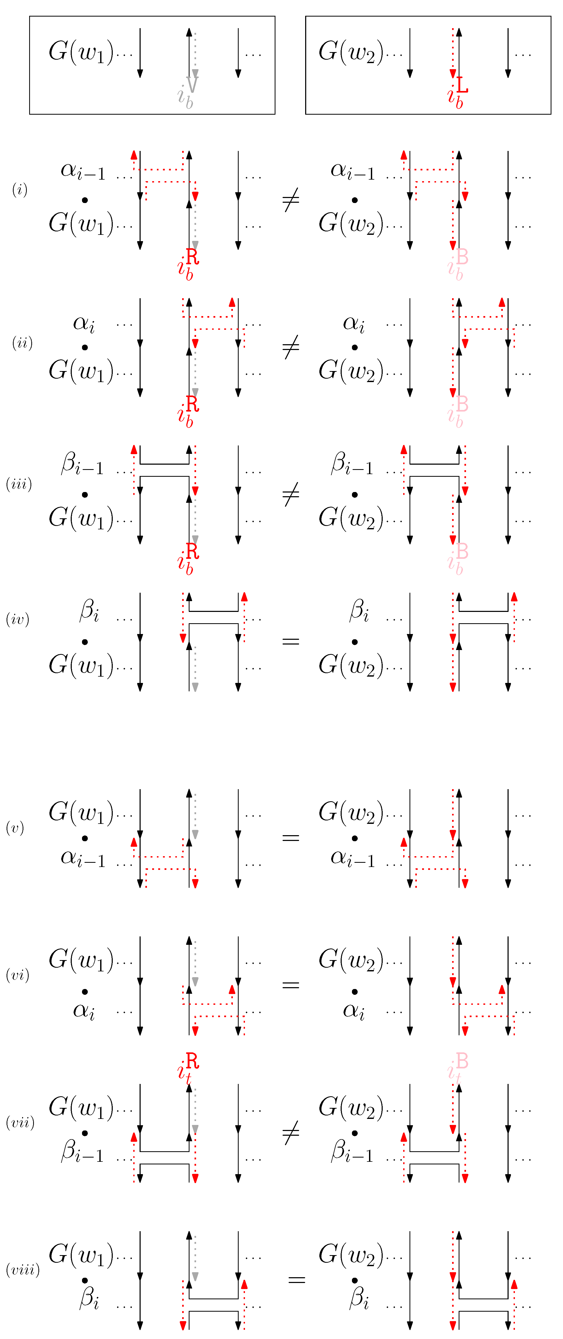
  When $s\left(i\right)$ is virtual and $r\left(i\right)$ is left: We consider $\left(s\left(i\right)=(i_t^{\mathtt{V}},i_b^{\mathtt{V}}),(s\left(i\right)=i_t^{\mathtt{L}},i_b^{\mathtt{L}})\right)$ for odd is in Figure 11. We establish the following override set: $O_{\mathtt{V}\mathtt{L}}\left(i\right)=\left\{({\beta }_{i}v,ϵ)\right\}\cup$ $\left\{(ϵ,vz)\mid z\in \{{\alpha }_{i-1},{\alpha }_i,{\beta }_i\}\right\}\cup \left\{({\alpha }_{i-1}v,w_{⊐}^{\prime })\mid (ϵ,w_{⊐}^{\prime })\in O_{cap}\left(i\right)\right\}\cup$ $\left\{({\alpha }_{i}v,w_{⊐}^{\prime })\mid (ϵ,w_{⊐}^{\prime })\in O_{cap}(i+1)\right\}\cup \left\{(w_{⊏}^{\prime }{\beta }_{i-1},w_{⊐}^{\prime }),(w_{⊏}^{\prime },{\beta }_{i-1}{w}_{⊐}^{\prime })\mid (w_{⊏}^{\prime },w_{⊐}^{\prime })\in O_{\mathtt{R}\mathtt{B}}\left(i\right)\right\}$ for $Z=\{{\alpha }_{i-1},{\alpha }_i,{\beta }_{i-1},{\beta }_i\}$ and $v\in {({\Sigma }_n\setminus Z)}^{*}$.

  (e)

  When $s\left(i\right)$ is virtual and $r\left(i\right)$ is block: We consider $\left(s\left(i\right)=(i_t^{\mathtt{V}},i_b^{\mathtt{V}}),r\left(i\right)=(i_t^{\mathtt{B}},i_b^{\mathtt{B}})\right)$ for odd is in Figure 12. We establish the following override set: $O_{\mathtt{V}\mathtt{B}}\left(i\right)=\left\{({\beta }_{i}v,ϵ),(ϵ,v{\beta }_i)\right\}\cup \left\{({\alpha }_{i-1}v,w_{⊐}^{\prime })\mid (ϵ,w_{⊐}^{\prime })\in O_{cap}\left(i\right)\right\}$ $\cup \left\{({\alpha }_{i}v,w_{⊐}^{\prime })\mid (ϵ,w_{⊐}^{\prime })\in O_{cap}(i+1)\right\}\cup \left\{(w_{⊏}^{\prime },v{\alpha }_{i-1})\mid (w_{⊏}^{\prime },ϵ)\in O_{cup}\left(i\right)\right\}\cup \left\{(w_{⊏}^{\prime },v{\alpha }_i)\mid (w_{⊏}^{\prime },ϵ)\in O_{cup}(i+1)\right\}$ $\cup \left\{(w_{⊏}^{\prime }{\beta }_{i-1},w_{⊐}^{\prime }),(w_{⊏}^{\prime },{\beta }_{i-1}{w}_{⊐}^{\prime })\mid (w_{⊏}^{\prime },w_{⊐}^{\prime })\in O_{\mathtt{R}\mathtt{B}}\left(i\right)\right\}$ for $Z=\{{\alpha }_{i-1},{\alpha }_i,{\beta }_{i-1},{\beta }_i\}$ and $v\in {({\Sigma }_n\setminus Z)}^{*}$.

Note that the definition of each override set only refers to the previously defined override sets. We reorganize the override sets by substitution:

• $O_{cap}\left(i\right)=\left\{(ϵ,vz)\mid v\in {({\Sigma }_n\setminus Z)}^{*},z\in Z\right\}$ for $Z=\{{\alpha }_{i-2},{\alpha }_{i-1},{\alpha }_i,{\beta }_{i-1},{\beta }_i\}$.
• $O_{cup}\left(i\right)=\left\{(zv,ϵ)\mid v\in {({\Sigma }_n\setminus Z)}^{*},z\in Z\right\}$ for $Z=\{{\alpha }_{i-2},{\alpha }_{i-1},{\alpha }_i,{\beta }_{i-2},{\beta }_{i-1}\}$.
• $O_{\mathtt{R}\mathtt{B}}\left(i\right)=\left\{({\beta }_{i}v\left[1\right],ϵ),(ϵ,v\left[1\right]z\left[1\right]),({\alpha }_{i-1}v\left[1\right],v\left[2\right]z\left[2\right]),({\alpha }_{i}v\left[1\right],v\left[3\right]z\left[3\right])\right\}$ for $Z\left[1\right]=\{{\alpha }_{i-1},{\alpha }_i,{\beta }_i\}$, $Z\left[2\right]=\{{\alpha }_{i-2},{\alpha }_{i-1},{\alpha }_i,{\beta }_{i-1},{\beta }_i\}$, $Z\left[3\right]=\{{\alpha }_{i-1},{\alpha }_i,{\alpha }_{i+1},{\beta }_i,{\beta }_{i+1}\}$, $z\left[j\right]\in Z\left[j\right]$ and $v\left[j\right]\in {({\Sigma }_n\setminus Z\left[j\right])}^{*}$ for $1\le j\le 3$.
• $O_{\mathtt{L}\mathtt{B}}\left(i\right)=\left\{(z\left[1\right]v\left[1\right],ϵ),(ϵ,v\left[1\right]{\beta }_{i-1}),(z\left[2\right]v\left[2\right],v\left[1\right]{\alpha }_{i-1}),(z\left[3\right]v\left[3\right],v\left[1\right]{\alpha }_i)\right\}$ for $Z\left[1\right]=\{{\alpha }_{i-1},{\alpha }_i,{\beta }_{i-1}\}$, $Z\left[2\right]=\{{\alpha }_{i-2},{\alpha }_{i-1},{\alpha }_i,{\beta }_{i-2},{\beta }_{i-1}\}$, $Z\left[3\right]=\{{\alpha }_{i-1},{\alpha }_i,{\alpha }_{i+1},{\beta }_{i-1},{\beta }_i\}$, $z\left[j\right]\in Z\left[j\right]$ and $v\left[j\right]\in {({\Sigma }_n\setminus Z\left[j\right])}^{*}$ for $1\le j\le 3$.
• $O_{\mathtt{V}\mathtt{R}}\left(i\right)=\{(z\left[4\right]v\left[1\right],ϵ),(ϵ,v\left[1\right]{\beta }_{i-1}),(z\left[2\right]v\left[2\right],v\left[1\right]{\alpha }_{i-1}),(z\left[3\right]v\left[3\right],v\left[1\right]{\alpha }_i),$
  $(z\left[4\right]v\left[4\right]{\beta }_i,ϵ),(z\left[4\right]v\left[4\right],{\beta }_i),({\beta }_i,v\left[4\right]{\beta }_{i-1}),(ϵ,{\beta }_{i}v\left[4\right]{\beta }_{i-1}),(z\left[2\right]v\left[2\right]{\beta }_i,v\left[4\right]{\alpha }_{i-1}),$
  $(z\left[2\right]v\left[2\right],{\beta }_{i}v\left[4\right]{\alpha }_{i-1}),(z\left[3\right]v\left[3\right]{\beta }_i,v\left[4\right]{\alpha }_i),(z\left[3\right]v\left[3\right],{\beta }_{i}v\left[4\right]{\alpha }_i)\}$ for $Z\left[1\right]=\{{\alpha }_{i-1},{\alpha }_i,{\beta }_{i-1},{\beta }_i\}$, $Z\left[2\right]=\{{\alpha }_{i-2},{\alpha }_{i-1},{\alpha }_i,{\beta }_{i-2},{\beta }_{i-1}\}$, $Z\left[3\right]=\{{\alpha }_{i-1},{\alpha }_i,{\alpha }_{i+1},{\beta }_{i-1},{\beta }_i\}$, $Z\left[4\right]=\{{\alpha }_{i-1},{\alpha }_i,{\beta }_{i-1}\}$, $z\left[j\right]\in Z\left[j\right]$ and $v\left[j\right]\in {({\Sigma }_n\setminus Z\left[j\right])}^{*}$ for $1\le j\le 4$.
• $O_{\mathtt{V}\mathtt{L}}\left(i\right)=\{({\beta }_{i}v\left[1\right],ϵ),(ϵ,v\left[4\right]z\left[1\right]),({\alpha }_{i-1}v\left[1\right],v\left[2\right]z\left[2\right]),({\alpha }_{i}v\left[1\right],v\left[3\right]z\left[3\right]),$
  $({\beta }_{i}v\left[4\right]{\beta }_{i-1},ϵ),({\beta }_{i}v\left[4\right],{\beta }_{i-1}),({\beta }_{i-1},v\left[4\right]z\left[4\right]),(ϵ,{\beta }_{i-1}v\left[4\right]z\left[4\right]),({\alpha }_{i-1}v\left[4\right]{\beta }_{i-1},v\left[2\right]z\left[2\right]),({\alpha }_{i-1}v\left[4\right],{\beta }_{i-1}v\left[2\right]z\left[2\right]),$
  $({\alpha }_{i}v\left[4\right]{\beta }_{i-1},v\left[3\right]z\left[3\right]),({\alpha }_{i}v\left[4\right],{\beta }_{i-1}v\left[3\right]z\left[3\right])\}$
  for $Z\left[1\right]=\{{\alpha }_{i-1},{\alpha }_i,{\beta }_{i-1},{\beta }_i\}$, $Z\left[2\right]=\{{\alpha }_{i-2},{\alpha }_{i-1},{\alpha }_i,{\beta }_{i-1},{\beta }_i\}$,
  $Z\left[3\right]=\{{\alpha }_{i-1},{\alpha }_i,{\alpha }_{i+1},{\beta }_i,{\beta }_{i+1}\}$, $Z\left[4\right]=\{{\alpha }_{i-1},{\alpha }_i,{\beta }_i\}$, $z\left[j\right]\in Z\left[j\right]$ and $v\left[j\right]\in {({\Sigma }_n\setminus Z\left[j\right])}^{*}$ for $1\le j\le 4$.
• $O_{\mathtt{V}\mathtt{B}}\left(i\right)=\{({\beta }_{i}v\left[1\right],ϵ),(ϵ,v\left[1\right]{\beta }_i),({\alpha }_{i-1}v\left[1\right],v\left[2\right]z\left[2\right]),({\alpha }_{i}v\left[1\right],v\left[3\right]z\left[3\right]),(z\left[4\right]v\left[4\right],v\left[1\right]{\alpha }_{i-1}),$
  $(z\left[5\right]v\left[5\right],v\left[1\right]{\alpha }_i),({\beta }_{i}v\left[6\right]{\beta }_{i-1},ϵ),({\beta }_{i}v\left[6\right],{\beta }_{i-1}),({\beta }_{i-1},v\left[6\right]z\left[6\right]),(ϵ,{\beta }_{i-1}v\left[6\right]z\left[6\right]),({\alpha }_{i-1}v\left[6\right]{\beta }_{i-1},v\left[2\right]z\left[2\right]),$
  $({\alpha }_{i-1}v\left[6\right],{\beta }_{i-1}v\left[2\right]z\left[2\right]),({\alpha }_{i}v\left[6\right]{\beta }_{i-1},v\left[3\right]z\left[3\right]),({\alpha }_{i}v\left[6\right],{\beta }_{i-1}v\left[3\right]z\left[3\right])\}$ for $Z\left[1\right]=\{{\alpha }_{i-1},{\alpha }_i,{\beta }_{i-1},{\beta }_i\}$,
  $Z\left[2\right]=\{{\alpha }_{i-2},{\alpha }_{i-1},{\alpha }_i,{\beta }_{i-1},{\beta }_i\}$, $Z\left[3\right]=\{{\alpha }_{i-1},{\alpha }_i,{\alpha }_{i+1},{\beta }_i,{\beta }_{i+1}\}$,
  $Z\left[4\right]=\{{\alpha }_{i-2},{\alpha }_{i-1},{\alpha }_i,{\beta }_{i-2},{\beta }_{i-1}\}$, $Z\left[5\right]=\{{\alpha }_{i-1},{\alpha }_i,{\alpha }_{i+1},{\beta }_{i-1},{\beta }_i\}$, $Z\left[6\right]=\{{\alpha }_{i-1},{\alpha }_i,{\beta }_i\}$,
  $z\left[j\right]\in Z\left[j\right]$ and $v\left[j\right]\in {({\Sigma }_n\setminus Z\left[j\right])}^{*}$ for $1\le j\le 6$.

Now, we inspect the rules in $R_{max}\left(n\right)$ to construct $R_e\left(n\right)$.

• ${\gamma }_i\overline{{\gamma }_j}\leftrightarrow \overline{{\gamma }_j}{\gamma }_i$: When $|i-j|\ge 2$, the rule also holds under ${\mathcal{G}}_e\left(n\right)$.

  (a)

  When $j=i+1$ and $\gamma =\alpha$, we observe that the only difference in graphical structures is the ith cap. Thus, ${\alpha }_i{\beta }_{i+1}{w}_{⊐}\leftrightarrow {\beta }_{i+1}{\alpha }_i{w}_{⊐}$ holds for $(ϵ,w_{⊐})\in O_{cap}\left(i\right)$.

  (b)

  When $j=i+1$ and $\gamma =\beta$, we observe that the only difference in graphical structures is the $i+1$st cup. Thus, $w_{⊏}{\beta }_i{\alpha }_{i+1}\leftrightarrow w_{⊏}{\alpha }_{i+1}{\beta }_i$ holds for $(w_{⊏},ϵ)\in O_{cup}(i+1)$.

  (c)

  When $i=j$, we observe that there are $i+1$st cup and cap differences. Thus, $w_{⊏}{\alpha }_i{\beta }_i{w}_{⊐}\leftrightarrow w_{⊏}{\beta }_i{\alpha }_i{w}_{⊐}$ holds for $(w_{⊏},ϵ)\in O_{cup}(i+1)$ and $(ϵ,w_{⊐})\in O_{cap}(i+1)$.

• ${\gamma }_i{\gamma }_i\leftrightarrow {\gamma }_i$: This rule also holds under ${\mathcal{G}}_e\left(n\right)$.
• ${\gamma }_i{\gamma }_j\leftrightarrow {\gamma }_j{\gamma }_i$ for $|i-j|\ge 2$: This rule also holds under ${\mathcal{G}}_e\left(n\right)$.
• ${\gamma }_i{\gamma }_j{\gamma }_i\leftrightarrow {\gamma }_i$ for $|i-j|=1$

  (a)

  When $\gamma =\alpha$ and $j=i-1$, we observe that the only difference in graphical structures is the ith straight virtual/block staples. Thus, $w_{⊏}{\alpha }_i{w}_{⊐}\leftrightarrow w_{⊏}{\alpha }_i{\alpha }_{i-1}{\alpha }_i{w}_{⊐}$ holds for $(w_{⊏},w_{⊐})\in O_{\mathtt{V}\mathtt{B}}(i-1)$.

  (b)

  When $\gamma =\alpha$ and $j=i+1$, we observe that the only difference in graphical structures is the $i+2$nd straight virtual/block staples. Thus, $w_{⊏}{\alpha }_i{w}_{⊐}\leftrightarrow w_{⊏}{\alpha }_i{\alpha }_{i+1}{\alpha }_i{w}_{⊐}$ holds for $(w_{⊏},w_{⊐})\in O_{\mathtt{V}\mathtt{B}}(i+2)$.

  (c)

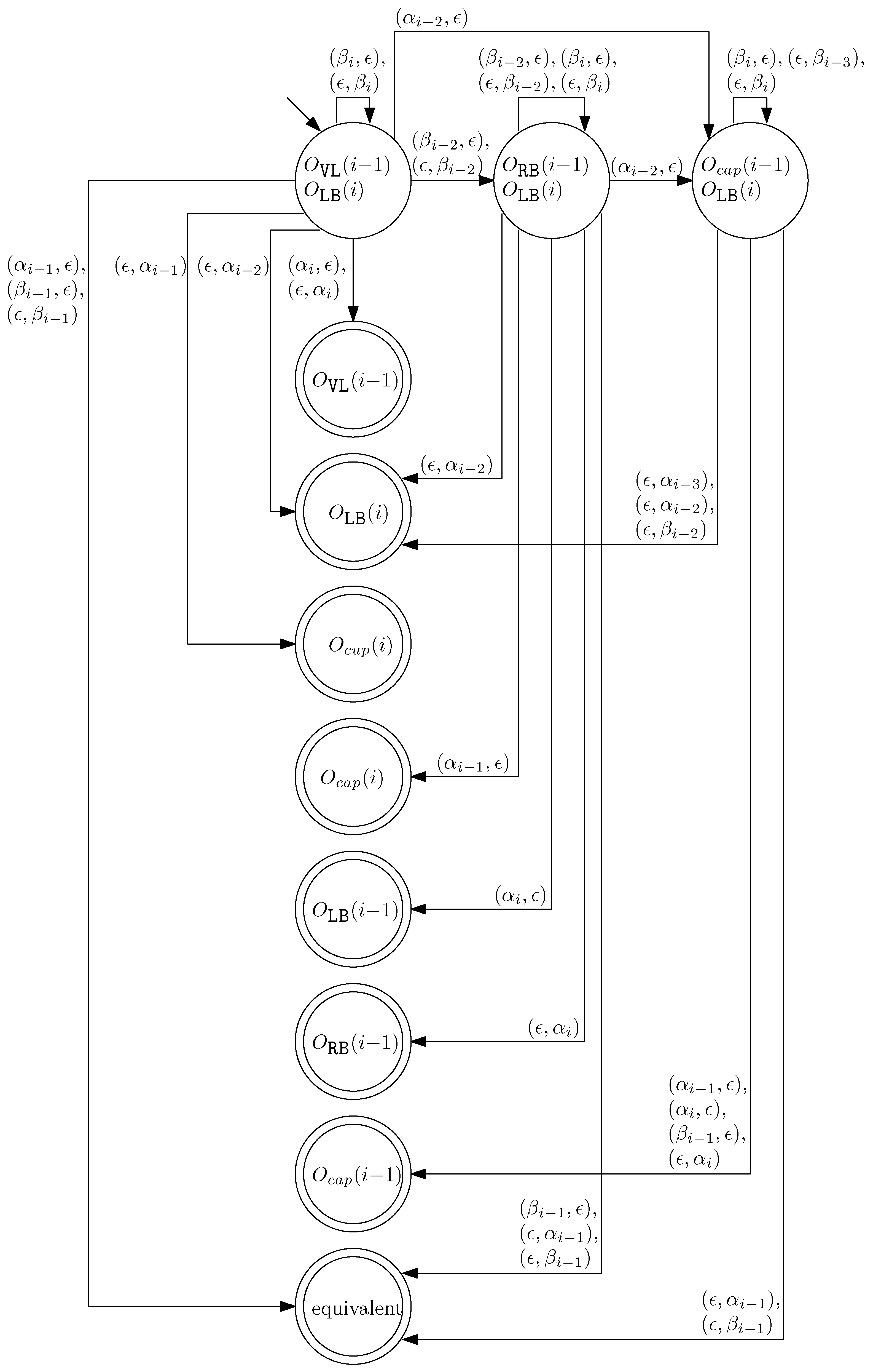
  When $\gamma =\beta$ and $j=i-1$, we observe that the differences in graphical structures are the $i-1$st straight virtual/block staple and the ith straight left/block staple. Since straight differences on two adjacent columns can become the same by simply applying $O_{\mathtt{V}\mathtt{B}}(i-1)$ and $O_{\mathtt{L}\mathtt{B}}$, we attach generators that affect the different staple types and observe the changes on the differences. Figure 13 illustrates the transition graph of the changes in the different staple types. Each node denotes the different staple types by override sets for the differences, and each transition has a set of pairs of a prefix and a suffix that changes the different staple types. Nodes with less than or equal to one type difference are double-circled to denote the “final” nodes, since we can directly apply the override set on the node to make two graphical structures equivalent. For $G\left({\beta }_i\right)$ and $G\left({\beta }_i{\beta }_{i-1}{\beta }_i\right)$, we start from the node with two override sets $O_{\mathtt{V}\mathtt{B}}(i-1)$ and $O_{\mathtt{L}\mathtt{B}}\left(i\right)$. Then, for example, if we follow transitions $({\alpha }_{i-2},ϵ)$ and $(ϵ,{\alpha }_{i-3})$, the resulting node has one override set $O_{\mathtt{L}\mathtt{B}}\left(i\right)$. From this sequence of transitions, we establish the rewriting rule $w_{⊏}{\alpha }_{i-2}v\left[1\right]{\beta }_{i}v\left[2\right]{\alpha }_{i-3}{w}_{⊐}\leftrightarrow w_{⊏}{\alpha }_{i-2}v\left[1\right]{\beta }_i{\beta }_{i-1}{\beta }_{i}v\left[2\right]{\alpha }_{i-3}{w}_{⊐}$ for $v\left[1\right]\in {({\Sigma }_n\setminus \{{\alpha }_{i-1},{\alpha }_i,{\beta }_{i-2},{\beta }_{i-1},{\beta }_i\})}^{*}$, $v\left[2\right]\in {({\Sigma }_n\setminus \{{\alpha }_{i-2},{\alpha }_{i-1},{\alpha }_i,{\beta }_{i-3},{\beta }_{i-2},{\beta }_{i-1},{\beta }_i\})}^{*}$ and $(w_{⊏},w_{⊐})\in O_{\mathtt{L}\mathtt{B}}\left(i\right)$. In general, we can recursively construct a rewriting rule based on a sequence of transitions that leads to a final node as follows:

  • We start with $w_1={\beta }_i$ and $w_2={\beta }_i{\beta }_{i-1}{\beta }_i$ and the current node with two override sets $O_{\mathtt{V}\mathtt{B}}(i-1)$ and $O_{\mathtt{L}\mathtt{B}}\left(i\right)$.
  • For a transition $(\zeta ,ϵ)$ from the current node, append a prefix $\zeta v$ to $w_1$ and $w_2$ where v does not have any ${\zeta }^{\prime }$ such that the transition $({\zeta }^{\prime },ϵ)$ exists from the current node.
  • For a transition $(ϵ,\zeta )$ from the current node, append a suffix $v\zeta$ to $w_1$ and $w_2$ where v does not have any ${\zeta }^{\prime }$ such that the transition $(ϵ,{\zeta }^{\prime })$ exists from the current node.
  • Update the current node by following the transition. If the current node is final with the override set O, we establish the rewriting rule $w_{⊏}{w}_1{w}_{⊐}\leftrightarrow w_{⊏}{w}_2{w}_{⊐}$ for $(w_{⊏},w_{⊐})\in O$. Otherwise, repeat the process from the current node.

  (d)

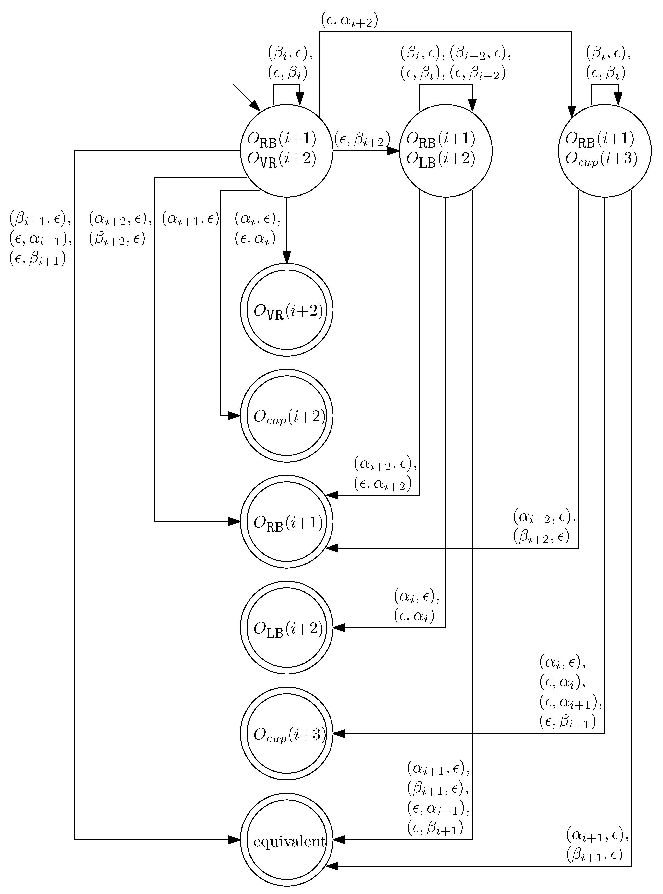
  When $\gamma =\beta$ and $j=i+1$, we can similarly construct the transition graph as Figure 14. Based on this transition graph, we can recursively construct a set of rewriting rules.

Note that the transition graphs in Figure 13 and Figure 14 are not symmetric with respect to the indices (i.e., changing index j to $2i+1-j$ from Figure 13 does not construct Figure 14).

We union the sets of previously analyzed rewriting rules to construct $R_e\left(n\right)$. It is straightforward that if $w_1\sim w_2$ under $R_e\left(n\right)$, then $G\left(w_1\right)=G\left(w_2\right)$ under ${\mathcal{G}}_e\left(n\right)$. Moreover, since $R_e\left(n\right)$ is constructed from recursively tracing every possible difference in the graphical structures of $G\left(w_1\right)$ and $G\left(w_2\right)$ where $G\left(w_1\right)=G\left(w_2\right)$ under ${\mathcal{G}}_{max}\left(n\right)$, the converse of the statement also holds: if $G\left(w_1\right)=G\left(w_2\right)$ under ${\mathcal{G}}_e\left(n\right)$, then $w_1\sim w_2$ under $R_e\left(n\right)$. Based on $R_e\left(n\right)$, we can also define ${\mathcal{O}}_e\left(n\right)$, the set of equivalent classes under ${\widehat{R}}_e\left(n\right)$.

4.2. Properties of Graphical Structures and Equivalent Classes

Here, we inspect the properties of graphical structures under ${\mathcal{G}}_e\left(n\right)$, which we will use to count the number of distinct equivalent classes. For two graphical structures $G\left(w\right)=(\mathcal{C},\mathcal{P})$ and $G\left(w^{\prime }\right)=({\mathcal{C}}^{\prime },{\mathcal{P}}^{\prime })$, we say that $G\left(w\right)$ is isomorphic to $G\left(w^{\prime }\right)$ (and vice versa) if there exists one-to-one correspondence between scaffolds in $\mathcal{C}$ and ${\mathcal{C}}^{\prime }$ (staples in $\mathcal{P}$ and ${\mathcal{P}}^{\prime }$) with the same pair of endpoints. For instance, if we compare the graphical structures from the same word under ${\mathcal{G}}_e\left(n\right)$ and ${\mathcal{G}}_{max}\left(n\right)$, one is isomorphic to the other—the only difference is the four different types of staples (virtual, left, right, block) under ${\mathcal{G}}_e\left(n\right)$. However, not all combinations of these types of staples are realizable under ${\mathcal{G}}_e\left(n\right)$. We first analyze the possible combinations of different types of staples. Then, for each given graphical structure $G\left(w\right)$ under ${\mathcal{G}}_{max}\left(n\right)$, we count the number of distinct graphical structures under ${\mathcal{G}}_e\left(n\right)$ that are isomorphic to $G\left(w\right)$.

For further analysis of staples, we first define four different types of a column according to the scaffold structure. For a given graphical structure, the ith column can be categorized into four different types:

• Straight if there exists a straight scaffold on the ith column.
• Crossing if there exists a scaffold from the jth column to the kth column such that $j<i<k$ or $k<i<j$ holds.
• Left-sided if the ith column is not crossing and all scaffolds with endpoints on the ith column have the other endpoints on the jth column such that $j<i$.
• Right-sided if the ith column is not crossing and all scaffolds with endpoints on the ith column have the other endpoints on the jth column such that $i<j$.

Since each position is assigned to distinct endpoints of scaffolds and there is no crossing of scaffolds, these four different types partition the set of all columns.

Lemma 1. 

For given graphical structure $G\left(w\right)$ under ${\mathcal{G}}_e\left(n\right)$, staples in $G\left(w\right)$ have the following properties:

• If a staple is virtual straight, then the staple is on a straight column.
• If a staple is a cup, then the staple is left or block.
• If a staple is a cap, then the staple is right or block.
• If a staple is left straight, then the staple is on a straight or right-sided column.
• If a staple is right straight, then the staple is on a straight or left-sided column.
• If a staple is not a cap/a cup/a straight segment, then the staple is block.

Lemma 2. 

For given graphical structure $G\left(w\right)$ under ${\mathcal{G}}_e\left(n\right)$, there always exists a graphical structure $G\left(w^{\prime }\right)$ under ${\mathcal{G}}_e\left(n\right)$ that satisfies the following properties:

• $G\left(w^{\prime }\right)$ is isomorphic to $G\left(w\right)$.
• A staple is virtual if and only if the staple is straight and on a straight column.
• If a staple is a cup, then the staple is left.
• If a staple is a cap, then the staple is right.
• A staple is left straight if and only if the staple is on a right-sided column.
• A staple is right straight if and only if the staple is on a left-sided column.

Proof of Lemma 2. 

Figure 15 gives an example of $G\left(w\right)$ and $G\left(w^{\prime }\right)$. □

We also observe that if ${\alpha }_i$ is in w, then the ith and the $i+1$st columns cannot have left or right straight staples.

We now classify graphical structures using a binary b of length n, where the ith digit has 1 if the ith column has a straight scaffold and 0 otherwise. The set of binaries of length n has bijection with the set ${\displaystyle T_{\left(\beta \right)n}=\{p=(a_1,b_1,\dots ,a_k,b_k)\mid k\ge 1,0\le a_1,b_k\le n,1\le a_i\le n,0\le b_i\le n\mathrm{for} \mathrm{all} i,\mathrm{and}\sum _{i=1}^k(a_i+b_i)=n\}}$. Thus, let $D\left(p\right)$ be the number of graphical structures which correspond to $p\in T_{\left(\beta \right)n}$.

Theorem 1. 

Given $n\in {\mathbb{N}}^0$, for each tuple ${\displaystyle p\in \bigcup _{1\le i\le n}{T}_{\left(\beta \right)i}}$, let $D\left(p\right)\in {\mathbb{N}}^0$ be recursively defined as follows:

• for $p\in T_{\left(\beta \right)0}$, $D(0,0)=1$.
• for $p\in T_{\left(\beta \right)1}$, $D\left(p\right)=1$ if $p=(0,1)$ and $D\left(p\right)=0$ if $p=(1,0)$.
• for $p=(a_1,b_1,\dots ,a_k,b_k)\in T_{\left(\beta \right)n}$, $(n>0)$ we have ${\displaystyle D\left(p\right)=\prod _{i=1}^{k}D(a_i,0)}$.
• for $n>1$, we have $D(0,n)=1$ and

  $$D(n,0)={\displaystyle \frac{1}{n+1}}\left({\displaystyle \genfrac{}{}{0pt}{}{2n}{n}}\right)-\sum _{p\in T_{\left(\beta \right)n}\setminus \left\{(n,0)\right\}}D\left(p\right).$$

Then, the size of the set of equivalent classes of words from ${\Sigma }_{\left(\beta \right)n}$ is given as

$${\displaystyle |{\mathcal{O}}_{\left(\beta \right)e}\left(n\right)|=\sum _{p\in T_{\left(\beta \right)n}}\left(D\left(p\right)\times x\left(p\right)\right)-n,}$$

where $x(a_1,b_1,\dots ,a_k,b_k)$ is given as

$${\displaystyle \sum _{p^{\prime }=(a_1^{\prime },b_1^{\prime },\dots ,a_l^{\prime },b_l^{\prime })\in T_{\left(\beta \right)k}}\left(\left(\prod _{i=1}^{l-1}{c}_i^{\prime }\right)·(b_{(s_l^{\prime }-b_l^{\prime })}+1)-1\right)}$$

for ${\displaystyle s_i^{\prime }=\sum _{j=1}^i(a_j^{\prime }+b_j^{\prime })}$ and $c_i^{\prime }=(b_{(s_i^{\prime }-b_i^{\prime })}+1)(b_{s_i^{\prime }}+1)$ if $b_i^{\prime }\ge 1$ and ${\displaystyle \frac{(b_{s_i^{\prime }}+1)(b_{s_i^{\prime }}+2)}{2}}$ if $b_i^{\prime }=0$.

Proof of Theorem 1. 

We observe that all staples in a graphical structure of a word from ${\Sigma }_{\left(\beta \right)n}$ are straight. Moreover, all straight staples are either left or right in the generators, and if the ith straight staple was block in $G\left(w\right)$, then the ith straight staple is block in all $G\left(uwv\right)$ where $u,w,v\in {\Sigma }_{\left(\beta \right)n}^{*}$. Thus, for each graphical structure, we first find a structure with the minimal block staples, and count the number of graphical structures with the same connectivity. It is straightforward to verify that $D(0,1)=1$ because there is only one case for $p=(0,1)$, while $D(1,0)=0$ since $p=(1,0)$ corresponds to an invalid case. For tuples $p=(a_1,b_1,\dots ,a_k,b_k)\in T_{\left(\beta \right)n}$, the columns with 1s in the binary representation always have only one possible case (straight scaffold and staple). Therefore, $D\left(p\right)$ is computed as the product of $D(a_i,0)$ for all i, that is:

$$D\left(p\right)=\prod _{i=1}^{k}D(a_i,0).$$

To calculate $D(a_1,0)$, we observe that the total number of graphical structures for $a_1$ is given by the Catalan number:

$$|{\mathcal{J}}_{a_1}|={\displaystyle \frac{1}{a_1+1}}\left({\displaystyle \genfrac{}{}{0pt}{}{2a_1}{a_1}}\right).$$

Using the recursive definition, $D(a_1,0)$ can be computed by summing over all valid tuples $p\in T_{\left(\beta \right)a_1}$:

$$|{\mathcal{J}}_{a_1}|=\sum _{p\in T_{\left(\beta \right)a_1}}D\left(p\right).$$

For $D(n,0)$, the value is determined by subtracting the contributions of all tuples $p\in T_{\left(\beta \right)n}\setminus \left\{(n,0)\right\}$ from the total number of structures:

$$D(n,0)={\displaystyle \frac{1}{n+1}}\left({\displaystyle \genfrac{}{}{0pt}{}{2n}{n}}\right)-\sum _{p\in T_{\left(\beta \right)n}\setminus \left\{(n,0)\right\}}D\left(p\right).$$

Finally, the size of the equivalence classes of words from ${\Sigma }_{\left(\beta \right)n}$ is given by:

$$|{\mathcal{O}}_{\left(\beta \right)e}\left(n\right)|=\sum _{p\in T_{\left(\beta \right)n}}\left(D\left(p\right)\times x\left(p\right)\right)-n,$$

where $x\left(p\right)$ is calculated recursively based on the tuples $p\in T_{\left(\beta \right)n}$. □

Given a graphical structure with n straight scaffolds, there exist the following different types of staple segment:

• a $cup$ if a staple segment $s=(i_t,j_t)$, where $0<|j-i|=1$,
• an $extendedcup$ if a staple segment $s=(i_t,j_t)$, where $0<|j-i|=2k+1$ for $1\le k$,
• a $cap$ if a staple segment $s=(i_t,j_t)$, where $0<|j-i|=1$
• an $extendedcap$ if a staple segment $s=(i_b,j_b)$, where $0<|j-i|=2k+1$ for $1\le k$,
• a $junction$ if a staple segment $s=(i_t,j_b)$, where $0<|j-i|=2k$ for $1\le k$.

Without loss of generality, we omit superscripts $\mathtt{B},\mathtt{L},\mathtt{R}$ that represent where two endpoints of the staple are placed on the scaffolds. Figure 16 shows the five different types of staple segment with n columns.

Given a graphical structure with n straight scaffolds, we define ${\parallel }_n$ to represent a set of staple segments over extended_cup, extended_cap, and junction that satisfy the following properties:

(i)

A bridge of width n is a subset of staple set $\mathcal{P}$ of the given graphical structure,

(ii)

For any staple segments $s=(i_p^d,j_q^d)$ in a bridge of width n, $|j-i|=2k$ for $k\ge 1$,

(iii)

For any staple segments $s=(i_p^d,j_p^d)$ in a bridge of width n, $|j-i|=2k+1$, for $k\ge 0$,

(iv)

A bridge of width n consequently spans n columns,

(v)

There is no proper subset of a bridge of width n which is a bridge of width n.

Given a graphical structure of width n, a staple segment $s=(i_p^d,j_q^d)$ of endpoints, where $p,q\in \{t,b\},d\in \{\mathtt{B},\mathtt{L},\mathtt{R}\}$, and $1\le i,j\le n$, spans columns from i to j if $i<j$ (or from the j to i if $j<i$).

We call a set of staple segments a bridge of width n if it satisfies the following properties (see Figure 17 for an example of a bridge of width n):

(i)

A bridge of width n is a subset of staple set $\mathcal{P}$ of the given graphical structure,

(ii)

For any staple segments $s=(i_p^d,j_q^d)$ in a bridge of width n, $|j-i|=2k$ for $k\ge 1$,

(iii)

For any staple segments $s=(i_p^d,j_p^d)$ in a bridge of width n, $|j-i|=2k+1$, for $k\ge 0$,

(iv)

A bridge of width n consequently spans n columns,

(v)

There is no proper subset of a bridge of width n which is a bridge of width n.

Figure 17. An example of a bridge of width n. (a) A set $\{(1_t^L,3_b^L),(5_t^L,2_t^L),(4_b^L,6_t^R)\}$ of staple segments is a bridge of width 6. (b) There exists a set $\{(1_t^L,5_b^R),(6_b^R,4_t^L),(4_b^R,1_b^L)\}$ that violates the property (v) since a proper subset $\{(6_b^R,4_t^L),(4_b^R,1_b^L)\}$ is a bridge of width 6. Therefore, the set $\{(1_t^L,5_b^R),(6_b^R,4_t^L),(4_b^R,1_b^L)\}$ is not bride of width 6 whereas the set $\{(1_t^L,5_b^L),(6_b^R,4_t^L)\}$ is a bridge. (c) A set $\{(1_t^L,3_b^R),(6_b^R,2_t^L)\}$ is a bridge of width 6. (d) A staple segment $(5_t^L,2_t^L)$ violates the property (ii) for a bridge of width 7. A set $\left\{(1_t^L,7_b^R)\right\}$ is a bridge of width 7.

Figure 17. An example of a bridge of width n. (a) A set $\{(1_t^L,3_b^L),(5_t^L,2_t^L),(4_b^L,6_t^R)\}$ of staple segments is a bridge of width 6. (b) There exists a set $\{(1_t^L,5_b^R),(6_b^R,4_t^L),(4_b^R,1_b^L)\}$ that violates the property (v) since a proper subset $\{(6_b^R,4_t^L),(4_b^R,1_b^L)\}$ is a bridge of width 6. Therefore, the set $\{(1_t^L,5_b^R),(6_b^R,4_t^L),(4_b^R,1_b^L)\}$ is not bride of width 6 whereas the set $\{(1_t^L,5_b^L),(6_b^R,4_t^L)\}$ is a bridge. (c) A set $\{(1_t^L,3_b^R),(6_b^R,2_t^L)\}$ is a bridge of width 6. (d) A staple segment $(5_t^L,2_t^L)$ violates the property (ii) for a bridge of width 7. A set $\left\{(1_t^L,7_b^R)\right\}$ is a bridge of width 7.

We define ${\parallel }_n$ to represent a set of all bridges of width n.

For a bridge of width n there are consecutive endpoints at the top and at the bottom which are not spanned by the bridge. For instance, there are consecutive endpoints $(2_t,\dots ,5_t)$ and $(1_b,\dots ,4_b)$ for a bridge $\left\{(1_t^L,5_b^R)\right\}$ of width 5.

We recall that a binary string of length n represents the graphical structures, and ${\displaystyle T_{\left(\alpha \right)n}=\{p\mid p=(a_1,b_1,\dots ,a_k,b_k),k\ge 1,0\le a_1,b_k\le n,1\le a_i,b_i\le n\mathrm{for} \mathrm{all} i,\mathrm{and}\sum _{i=1}^k(a_i+b_i)=n\}}$ denotes the set of tuples corresponding to the binary string.

Given a set of $2n$ positions, we calculate the number of partial graphical structures with t caps (or cups) as follows:

$$D(2n,t)=\sum _{n_1+\cdots +n_i=n,t_1+\cdots +t_i=t,n_j\ge t_j\ge 1\mathrm{for} \mathrm{all} j\le i}\prod _{j=1}^{i}D(2n_j-2,t_j)$$

with initial conditions $D(2,1)=D(0,1)=1$ and $D(2n,t)=0$ for all $n<t$.

5. Conclusions

This study presents a theoretical framework for side-aware DNA origami words, accounting for the directional attachment of staples to either the left or right side of the scaffold. This expansion of the traditional real and virtual staple classification to include left, right, virtual, and block types offers a more realistic representation of DNA origami structures, enabling the design of more intricate configurations.

We establish a rewriting system for side-aware DNA origami words and explore the properties of the corresponding graphical structures, with a focus on equivalence classes and rewriting patterns. Our model highlights the role of staple binding directionality in shaping the final structure, enhancing control over positioning and folding, which is crucial for applications in molecular devices and nanoscale assembly.

Although the complexity of rewriting rules in the ${\mathcal{G}}_{max\left(n\right)}$ case poses challenges for computational efficiency, future work will consider the ${\mathcal{G}}_{mid\left(n\right)}$ and ${\mathcal{G}}_{min\left(n\right)}$ contexts. These will help examine their impact on rewriting patterns and structural diversity, offering deeper insights into the role of virtual elements in DNA origami design. Additionally, identifying equivalence classes streamlines the design process by grouping structurally similar configurations, improving both the efficiency and flexibility of DNA origami structures. This classification is especially useful for optimizing stable designs and their applications in molecular devices and nanoscale assembly.

As a next step, we plan to validate the model through molecular simulations, specifically focusing on how structural width and staple types influence the overall shape. This will confirm the model’s accuracy and demonstrate its potential for real-world applications.

Finally, while this study focuses on 2D side-aware DNA origami, the framework can be extended to 3D structures. Addressing challenges related to staple orientation and computational efficiency will be key, and future work will explore these extensions to enable the design of more complex 3D DNA origami structures for advanced applications in molecular devices and nanoscale assembly.

References

- Whitesides, G.M.; Boncheva, M. Beyond Molecules: Self-assembly of mesoscopic and macroscopic components. Proc. Natl. Acad. Sci. USA 2002, 99, 4769–4774. [Google Scholar] [CrossRef] [PubMed]
- Evans, C.G.; Winfree, E. Physical principles for DNA tile self-assembly. Chem. Soc. Rev. 2017, 46, 3808–3829. [Google Scholar] [CrossRef] [PubMed]
- Winfree, E.; Eng, T.; Rozenberg, G. String Tile Models for DNA Computing by Self-Assembly. In Proceedings of the 6th International Workshop on DNA-Based Computers, Leiden, The Netherlands, 13–17 June 2000; pp. 63–88. [Google Scholar]
- Rothemund, P.W.K. Folding DNA to create nanoscale shapes and patterns. Nature 2006, 440, 297–302. [Google Scholar] [CrossRef] [PubMed]
- Garrett, J.; Jonoska, N.; Kim, H.; Saito, M. DNA origami words, graphical structures and their rewriting systems. Nat. Comput. 2021, 20, 217–231. [Google Scholar] [CrossRef]
- Zadegan, R.M.; Norton, M.L. Structural DNA nanotechnology: From design to applications. Int. J. Mol. Sci. 2012, 13, 7149–7162. [Google Scholar] [CrossRef] [PubMed]
- Kim, H.; Surwade, S.P.; Powell, A.; O’Donnell, C.; Liu, H. Stability of DNA Origami Nanostructure under Diverse Chemical Environments. Chem. Mater. 2014, 26, 5265–5273. [Google Scholar] [CrossRef]
- Voigt, N.V.; Tørring, T.; Rotaru, A.; Jacobsen, M.F.; Ravnsbæk, J.B.; Subramani, R.; Mamdouh, W.; Kjems, J.; Mokhir, A.; Besenbacher, F.; et al. Single-molecule chemical reactions on DNA origami. Nat. Nanotechnol. 2010, 5, 200–203. [Google Scholar] [CrossRef] [PubMed]
- Lin, C.; Liu, Y.; Rinker, S.; Yan, H. DNA tile based self-assembly: Building complex nanoarchitectures. ChemPhysChem 2006, 7, 1641–1647. [Google Scholar] [CrossRef] [PubMed]
- Douglas, S.M.; Dietz, H.; Liedl, T.; Högberg, B.; Graf, F.; Shih, W.M. Self-assembly of DNA into nanoscale three-dimensional shapes. Nature 2009, 459, 414–418. [Google Scholar] [CrossRef] [PubMed]
- Yin, P.; Hariadi, R.F.; Sahu, S.; Choi, H.M.T.; Park, S.H.; LaBean, T.H.; Reif, J.H. Programming DNA tube circumferences. Science 2008, 321, 824–826. [Google Scholar] [CrossRef]
- SantaLucia, J.; Allawi, H.T.; Seneviratne, P.A. Improved nearest-neighbor parameters for predicting DNA duplex stability. Biochemistry 1996, 35, 3555–3562. [Google Scholar] [CrossRef]
- Wei, B.; Dai, M.; Yin, P. Complex shapes self-assembled from single-stranded DNA tiles. Nature 2012, 485, 623–626. [Google Scholar] [CrossRef] [PubMed]
- Ke, Y.; Ong, L.L.; Shih, W.M.; Yin, P. Three-dimensional structures self-assembled from DNA bricks. Science 2012, 338, 1177–1183. [Google Scholar] [CrossRef] [PubMed]
- Adamczyk, A.K.; Huijben, T.A.P.M.; Sison, M.; Di Luca, A.; Chiarelli, G.; Vanni, S.; Brasselet, S.; Mortensen, K.I.; Stefani, F.D.; Pilo-Pais, M.; et al. DNA self-assembly of single molecules with deterministic position and orientation. ACS Nano 2022, 16, 16924–16931. [Google Scholar] [CrossRef] [PubMed]
- Lee, C.; Lee, J.Y.; Kim, D.-N. Polymorphic design of DNA origami structures through mechanical control of modular components. Nat. Commun. 2017, 8, 2067. [Google Scholar] [CrossRef] [PubMed]
- Ronald, V.B.; Friedrich, O. String-Rewriting Systems; Springer: Berlin/Heidelberg, Germany, 1993. [Google Scholar]
- Louis, H.K. Knots and Physics; World Scientific: Singapore, 2001. [Google Scholar]
- Borisavljević, M.; Došen, K.; Petric, Z. Kauffman Monoids. J. Knot Theory Its Ramif. 2002, 11, 127–143. [Google Scholar] [CrossRef]
- Lau, K.W.; FitzGerald, D.G. Ideal Structure of the Kauffman and Related Monoids. Commun. Algebra 2006, 34, 2617–2629. [Google Scholar] [CrossRef]
Disclaimer/Publisher’s Note: The statements, opinions and data contained in all publications are solely those of the individual author(s) and contributor(s) and not of MDPI and/or the editor(s). MDPI and/or the editor(s) disclaim responsibility for any injury to people or property resulting from any ideas, methods, instructions or products referred to in the content. |
© 2025 by the author. Licensee MDPI, Basel, Switzerland. This article is an open access article distributed under the terms and conditions of the Creative Commons Attribution (CC BY) license (https://creativecommons.org/licenses/by/4.0/).
Share and Cite
Cho, D.-J. Formalization of Side-Aware DNA Origami Words and Their Rewriting System, and Equivalent Classes. Mathematics 2025, 13, 895. https://doi.org/10.3390/math13060895
Cho D-J. Formalization of Side-Aware DNA Origami Words and Their Rewriting System, and Equivalent Classes. Mathematics. 2025; 13(6):895. https://doi.org/10.3390/math13060895
Chicago/Turabian StyleCho, Da-Jung. 2025. "Formalization of Side-Aware DNA Origami Words and Their Rewriting System, and Equivalent Classes" Mathematics 13, no. 6: 895. https://doi.org/10.3390/math13060895
APA StyleCho, D.-J. (2025). Formalization of Side-Aware DNA Origami Words and Their Rewriting System, and Equivalent Classes. Mathematics, 13(6), 895. https://doi.org/10.3390/math13060895