Abstract
Learning high-dimensional chaos is a complex and challenging problem because of its initial value-sensitive dependence. Based on an echo state network (ESN), we introduce homotopy transformation in topological theory to learn high-dimensional chaos. On the premise of maintaining the basic topological properties, our model can obtain the key features of chaos for learning through the continuous transformation between different activation functions, achieving an optimal balance between nonlinearity and linearity to enhance the generalization capability of the model. In the experimental part, we choose the Lorenz system, Mackey–Glass (MG) system, and Kuramoto–Sivashinsky (KS) system as examples, and we verify the superiority of our model by comparing it with other models. For some systems, the prediction error can be reduced by two orders of magnitude. The results show that the addition of homotopy transformation can improve the modeling ability of complex spatiotemporal chaotic systems, and this demonstrates the potential application of the model in dynamic time series analysis.
MSC:
68T07; 37M10
1. Introduction
In recent years, machine learning technologies have been widely applied to a variety of tasks, such as speech recognition, medical diagnosis, autonomous driving, image encryption and recommendation systems [1,2,3,4]. Chaos control has always been the focus of nonlinear research, and using machine learning technology to solve this problem has gradually become a trend [5,6,7,8]. We note that usually only finite time series data from certain dynamic processes are available. Thus, this method of learning only from the data itself is called “model-free” learning. The most commonly used method for model-free learning using dynamic time series is delayed coordinate embedding, which has been well established [9,10,11,12,13].
However, delayed coordinate embedding is too complex, and the results often fail to meet the accuracy required by the project. In 2004, the ESN proposed by Jaeger and Haas achieved impressive results in “model-free” chaotic learning tasks, which was published in Science [14]. In addition, many researchers have subsequently applied ESNs to various chaotic learning tasks. For example, Pathak et al. used reservoir computing to perform model-free estimates of the state evolution of chaotic systems and the Lyapunov exponents [15,16]. Moreover, ESN can also infer the unmeasured state variables from a limited set of continuously measured variables [17]. An ESN is very different from a traditional neural network; the difference is that an ESN only needs to train the output weight, and it overcomes the problem of gradient disappearance and explosion when the traditional neural network uses gradient descent on the weight matrix [18]. Therefore, In the following years, many results using ESNs have emerged [19]. For instance, adaptive reservoir computing can capture critical transitions in dynamical systems. This network has been successful in predicting critical transitions in various low-dimensional dynamical systems or high-dimensional systems with simple parameter structures [20]. Moreover, data-informed reservoir computing, which relies solely on data to enhance prediction accuracy, not only effectively reduces computational costs but also minimizes the cumbersome hyperparameter optimization process in reservoir computing [21].
The above results show that echo state networks can be effectively applied to chaos prediction tasks, and our goal is to achieve long-term and accurate predictions. However, chaotic systems are extremely sensitive to initial conditions, which makes long-term predictions more challenging. In the ESN structure, nonlinear activation can simulate the nonlinear relationship of the chaotic system, model data characteristics, and solve complex problems [22,23], so it is very important for the completion of the task.
The update process of the reservoir state largely depends on the activation function [24,25]. The activation function is a function of the network input, the previous state, and the feedback output. According to the reservoir update equation, the network input plays a crucial role in determining the reservoir state update. Different learning tasks involve distinct input characteristics, necessitating different reservoir update methods. However, in traditional ESN models, regardless of the characteristics of the input data, the activation function usually remains unchanged, typically using fixed nonlinear functions such as tanh or sigmoid [26]. Additionally, when noise or interference in the training set increases, the generalization ability of the ESN may decrease [27]. To overcome the shortcomings of traditional single activation functions, in recent years, the double activation function echo state network (DAF-ESN) [28], the echo state network activation function based on bistable stochastic resonance (SR-ESN) [29], and the deep echo state network with multiple activation functions (MAF-DESN) have been proposed [30]. By linearly combining activation functions, the resulting activation function varies as the coefficients change, providing greater flexibility and adaptability than single activation functions. This enhances the network’s expressive power, allowing the model to better adapt to complex learning tasks.
Recognizing this, in order to learn the key features of spatiotemporal chaotic systems, this paper introduces the homotopy transformation in topological theory and proposes a new chaotic prediction model, called the H-ESN. Under the premise of maintaining basic topological properties, our model achieves the optimal balance between nonlinearity and linearity by continuously transforming between different activation functions and adjusting the homotopy parameter, thereby capturing the key features necessary for learning chaos. In the experimental part of this paper, Our model has been successfully applied to the following classical prototype systems in chaotic dynamics: Lorenz system, MG system, and KS system, and it has obtained the following positive results compared to other models.
- With appropriately chosen parameters, the H-ESN can provide longer prediction times for various high-dimensional chaotic systems.
- Under the same parameter conditions, the H-ESN demonstrates smaller prediction errors compared to other models when predicting different dimensions of chaotic systems.
- Compared to traditional methods, the H-ESN exhibits significant advantages in chaotic prediction tasks, particularly in the estimation of the maximal Lyapunov exponent.
The remainder of this paper is organized as follows: Section 2 introduces the principles and methods of the ESN and H-ESN and provides the sufficient conditions for the H-ESN to satisfy the echo state property. Section 3 discusses the application of the H-ESN to three chaotic system examples and compares its performance with other models, achieving significant results. Section 4 summarizes our research findings and outlines future research directions.
2. Correlation Method
2.1. Echo State Network
The ESN, proposed by Jaeger and Haas, has a relatively simple structure and requires only a small number of parameter adjustments [31]. Compared to traditional neural networks, it trains just a portion of the network’s connection weights, specifically, the output weights, while the input weights and the weights of the recurrent connections within the reservoir are randomly generated and remain fixed [32,33]. This simplification makes the learning process faster and more efficient. It can significantly reduce computational costs and helps mitigate the vanishing gradient problem to some extent. Furthermore, when the number of reservoir nodes is much greater than one, we can expect a wide range of desired outputs. ESN is a machine learning framework that has been shown to reproduce the chaotic attractors of its dynamical systems and includes the fractal dimension and the Lyapunov exponential spectrum [34,35,36].
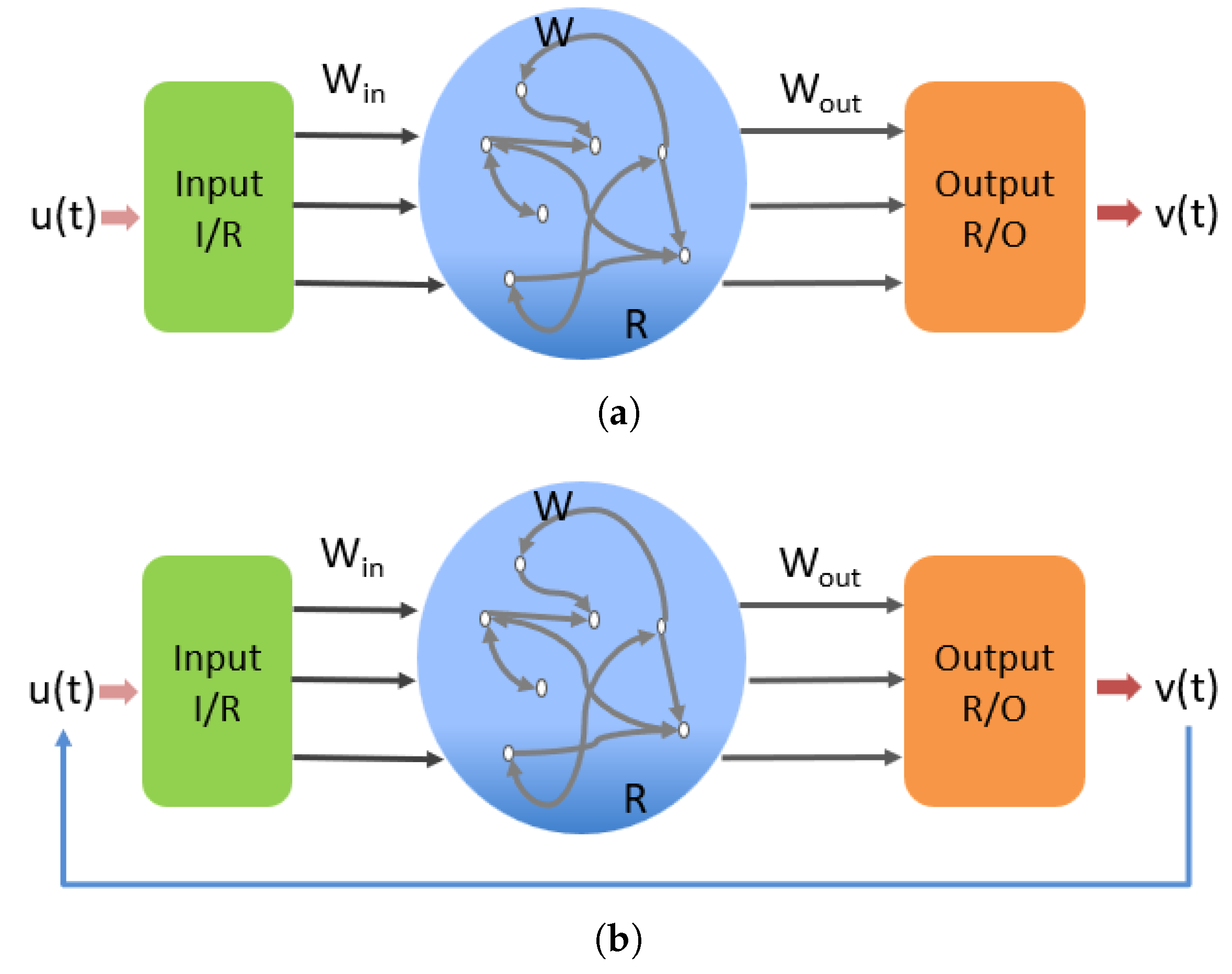
The operation of the ESN during the training phase is shown in Figure 1a; the D-dimensional input vector is mapped into the reservoir R with nodes via the input coupling and the input weight matrix . The reservoir state evolves according to Equation (1)
for the vector , the activation function tanh is expressed as (tanh(), tanh(), ⋯, tanh, which is the hyperbolic tangent function tanh(x). is the leakage rate, which adjusts the update speed of the reservoir states and affects the dynamic characteristics of the system. is the biased term, where . This introduces an additional degree of freedom to the reservoir, allowing the network to better fit complex nonlinear dynamic systems. In addition to and in Equation (1), the reservoir dynamics are also related to the spectral radius and sparsity d of the matrix . The spectral radius determines the stability and memory capacity of the reservoir, while the sparsity d influences the computational efficiency and dynamic diversity of the reservoir by controlling the proportion of non-zero elements in the matrix A. In Equation (2), is linearly combined with the -dimensional vector r(t) to obtain the output vector as follows

Figure 1.
Echo state network architecture: (a) training phase, and (b) testing phase. and denote the input-to-reservoir and reservoir-to-output couplers, respectively. denotes the reservoir.
Generally, the output v(t) obtained in Figure 1a is expected to approximate the desired output . During the training phase , the data for u(t) and are already known. The output weight matrix is determined by minimizing Equation (3) using ridge regression
where is the penalty parameter, is the sum of squares of each element, and the minimized loss function’s deduced as follows
After completing the training phase and obtaining the output weight matrix, the system enters the prediction phase . The desired method is to make the expected output equal to the input, i.e., , and after obtaining the output weight matrix, at , the system transitions from Figure 1a to Figure 1b and autonomously operates according to the following formula
2.2. Echo State Network Based on Homotopy Transformation (H-ESN)
2.2.1. Introduction to H-ESN
The activation function refers to the nonlinear function in neurons. The introduction of nonlinear characteristics into artificial neural networks improves the expression ability of the networks [37]. If a network lacks a nonlinear function, it can only perform linear combinations, making the activation function crucial in neural networks.
This section introduces an ESN model based on homotopy theory. The concept of homotopy originated from topological theory and has been applied to recovery algorithms. The core of the homotopy method lies in the use of continuous changing ideas and homotopy paths.
Theorem 1
([38]). Let be a continuous function on a topological space. A homotopy from f to g is a continuous function , such that for all and . If such a homotopy exists between f and g, then f is said to be homotopic to g for all . Denote this by . F is continuous on t, which means that the transformation from f to g is continuous, that is, the path from one function to another.
Theorem 2
([38]). Let C be a convex set. If for , then, there is , so we consider , because C is a convex set, so for any and for any , that is, a function from to C, so F is homotopy.
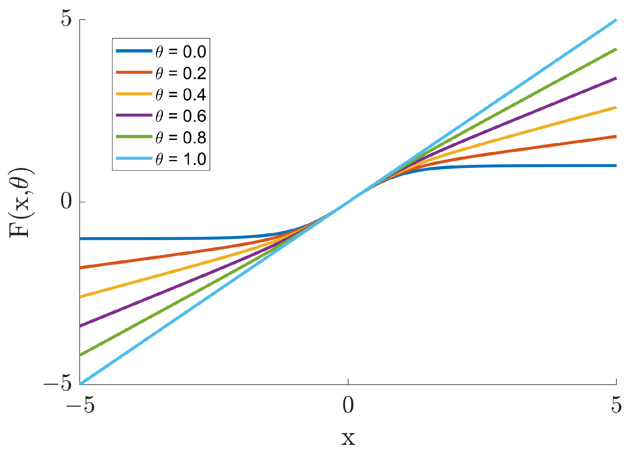
On the premise of maintaining the basic topological properties, our model can obtain the key features of chaos for learning through a continuous homotopy transformation between different activation functions. The activation function of our model is shown below
in which is the homotopy parameter. Figure 2 shows the graph of as the function transitions from to x for different values of .
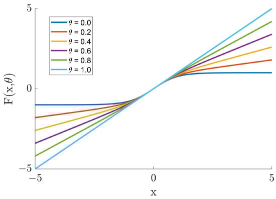
Figure 2.
Transition of from to x under different values of .
To provide a detailed explanation of the H-ESN training and prediction process, the specific flow of the algorithm, as well as its time and space complexity, are presented below (Algorithm 1).
| Algorithm 1 H-ESN standard algorithm process. |
|
2.2.2. Echo State Property of the H-ESN
The Echo State Property (ESP) is the core theoretical foundation of the ESN, ensuring that the dynamic behavior of the reservoir has good stability and predictability [39,40]. A sufficient condition for the H-ESN to exhibit the echo state property is given below (Table 1).

Table 1.
Time complexity and space complexity of the H-ESN algorithm.
Assumption 1.
The nonlinear activation function is a function from set X to set Y. There exists a constant such that for any two points in X, the Lipschitz condition is satisfied
where L is a constant, typically taken as 1.
Theorem 3.
If the following conditions are satisfied for the H-ESN model
- (1)
- (the parameter θ satisfies );
- (2)
- The spectral radius of the internal weight matrix A of the reservoir satisfies ;
The H-ESN model has the ESP.
Proof.
Consider two arbitrary initial states and , and the same input sequence . As , the state difference is . According to the state update equation
The tanh function is Lipschitz continuous, with a Lipschitz constant of 1.
3. Results
We will provide three examples, the Lorenz, Mackey–Glass, and Kuramoto–Sivashinsky systems, to illustrate the advantages of using the H-ESN in predicting chaotic systems.
3.1. Lorenz System
The Lorenz system, proposed by Edward Lorenz in 1963 [41], is a three-dimensional nonlinear dynamical system originally designed to study atmospheric convection. As a fundamental model in chaos theory, it is known for its simplicity and complex dynamics. The system’s differential equations are as follows
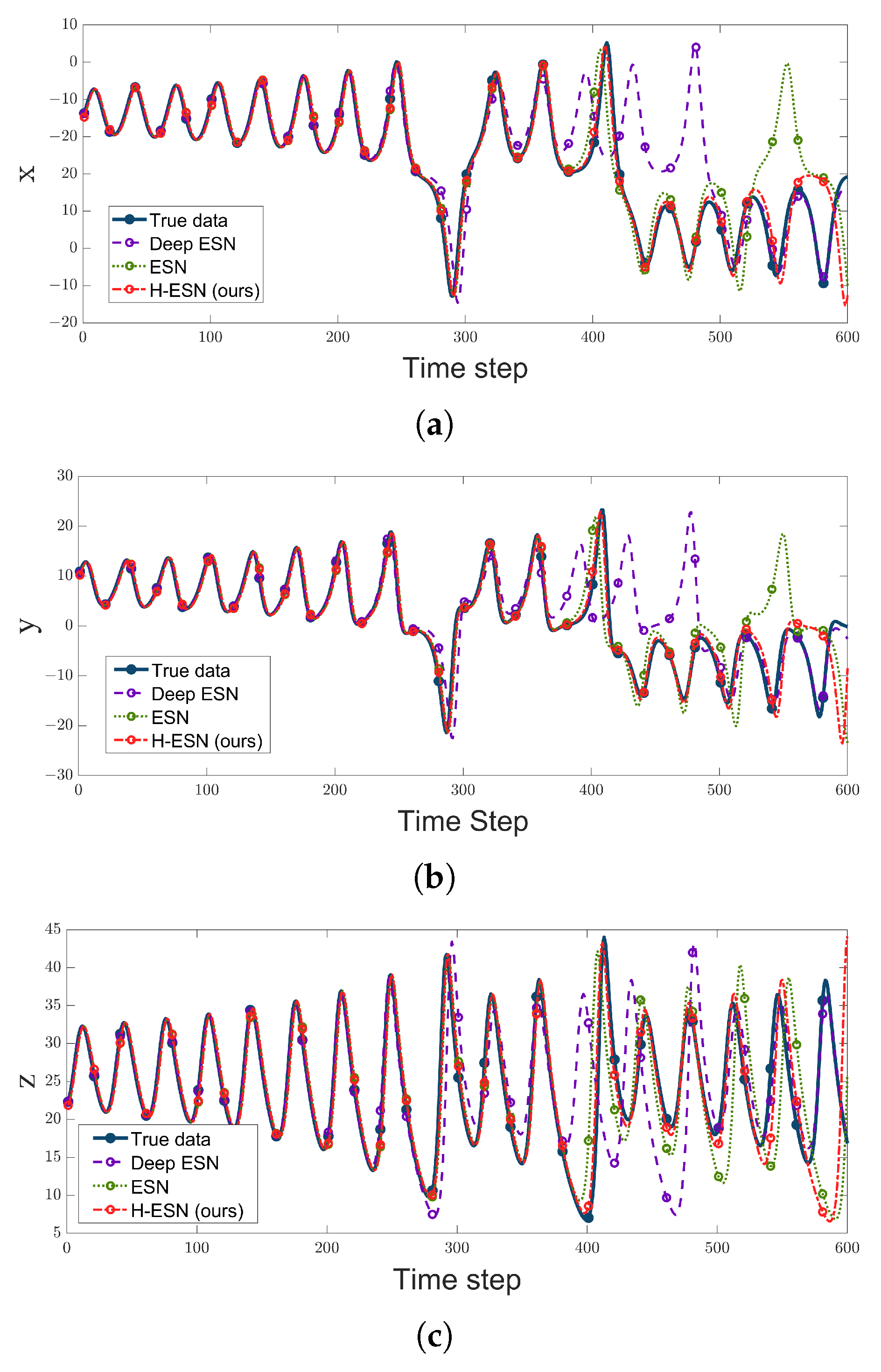
where and . The system variables are known, and the input is used to obtain the output weight matrix through training. Afterward, the system enters the prediction phase for . Taking into account the symmetry of the Lorenz equations, Equation (2) is modified to , where is a vector of dimensions in which half of the elements of are , with representing the components of . Based on this, we compare the H-ESN with other commonly used ESN models, and the results are illustrated in Figure 3, with the parameters shown in Table 2. Additionally, the accurate prediction data lengths for the three models on the three variables of the Lorenz system are presented in Table 3.
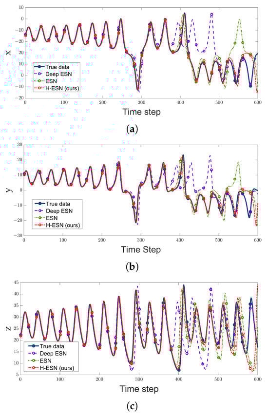
Figure 3.
Prediction results of the ESN, H-ESN, and DeepESN for each dimension of the Lorenz system. (a) Lorenz-x, (b) Lorenz-y, and (c) Lorenz-z.
Table 2.
Parameters for the Lorenz system prediction task.
Table 3.
Accurate prediction data lengths for the three variables of the Lorenz system using the ESN, Deep-ESN, and H-ESN.
According to Figure 3 and Table 3, in the initial stages, all three models—Deep ESN, ESN, and H-ESN—can achieve relatively accurate predictions for the three variables of the Lorenz system. However, as the number of data points increases, the prediction trajectory of the Deep ESN deviates first from the true values, with the purple dotted line diverging from the blue solid line. This is because we selected a Deep ESN with three layers, each containing 100 nodes, which results in weaker nonlinear modeling capability compared to an ESN with a single reservoir (300 nodes). Later, the predicted trajectory of the ESN also starts to deviate from the true state with an increase in data points, with the green dotted line moving away from the blue solid line. In contrast, H-ESN demonstrates a significant advantage in prediction duration compared to the other two models, achieving accurate predictions for approximately 500 data points for the three variables of the Lorenz system. For comparison, we computed the mean squared error (MSE) values of the three models for the three variables of the Lorenz system at different prediction lengths in Table 4.
Table 4.
Comparison table of MSE values for the three dimensions of the Lorenz system at different prediction lengths using the ESN, Deep ESN, and H-ESN.
As shown in Table 4, the MSE between the predicted values at 300, 350, 400, 450, and 500 data points and the true values of the three variables of the Lorenz system were calculated separately. Additionally, in Table 5, the average MSE percentage improvement of the H-ESN over the ESN for the three variables of the Lorenz system was calculated based on Equation (9). It can be concluded that the MSE value for the H-ESN model is minimal at different prediction stages, indicating that the model proposed in this paper achieves the best performance in this prediction task.
Table 5.
MSE percentage improvement of the H-ESN over the ESN.
In chaotic prediction tasks, the focus is on the duration and accuracy of predictions. Effective prediction time (EPT) is an important metric for evaluating the performance of time series prediction models. It refers to the limited period during which accurate predictions can be made using the model in chaotic scenarios. This period is finite because chaotic systems are extremely sensitive to initial conditions, leading to significant uncertainty in long-term predictions. In this paper, the effective prediction time is defined as . The prediction is considered invalid at time t, when the prediction error exceeds the set threshold , that is, when ( is a given error).
The parameter is a very important hyperparameter, and its selection significantly affects the system’s predictive performance. Figure 4 shows the EPT for the three variables under different values of . Overall, When is small, the EPT tends to decrease because the nonlinearity is too strong, making it difficult for the network to train or generalize effectively. When is large, the EPT also tends to decrease due to excessive linearization, causing the network to fail to capture the key dynamics of the chaotic system. However, after reaching the intermediate region at , the EPT starts to increase and reaches its maximum value, as the balance between nonlinearity and linearity is optimized. To ensure that the three variables have a longer prediction duration, it is recommended to choose a value of approximately 0.7.
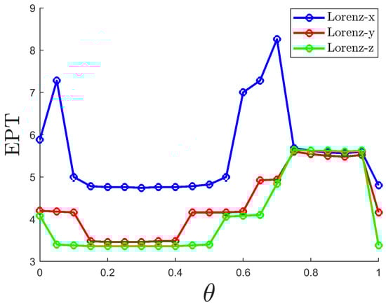
Figure 4.
EPT variation curves of the three dimensions of the Lorenz system with respect to are shown, with blue for Lorenz-x, red for Lorenz-y, and green for Lorenz-z.
The H-ESN introduces a linear component () through homotopy transformation, finding the optimal balance between nonlinearity and linearity. However, the value of generally varies for different chaotic systems. Currently, we primarily determine the value of through grid search or empirical tuning. While effective, this method can be computationally expensive when dealing with high-dimensional or complex systems. Finding the optimal value of quickly and efficiently is a major challenge faced by the H-ESN.
3.2. Mackey–Glass Equation
The Mackey–Glass (MG) equation is a commonly used delay differential equation used to model complex dynamic behaviors in biological and physical systems with time delays, especially in biology and ecology [42]. Its standard form is as follows
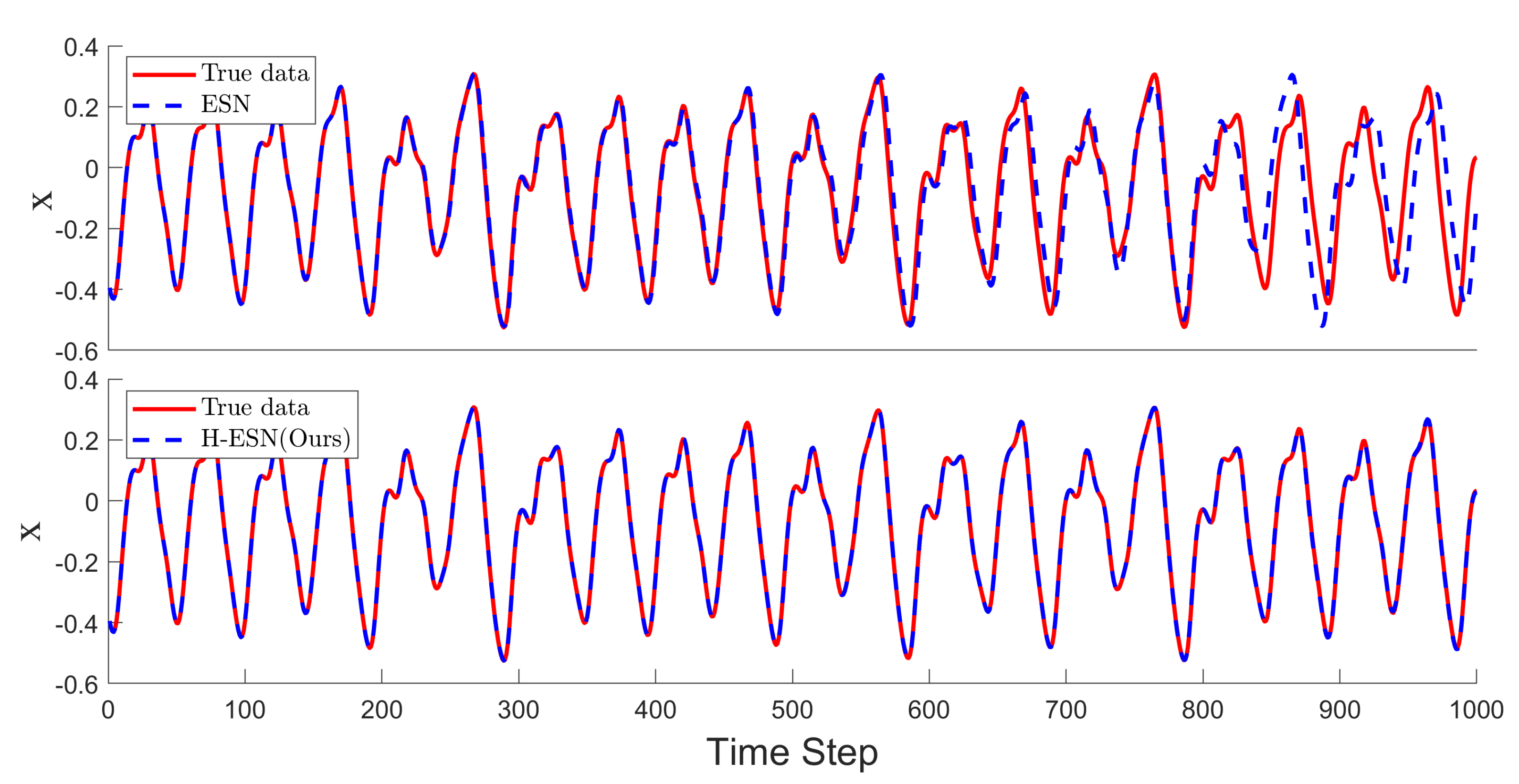
where = 0.2, = 0.1, = 17, and n = 10. The above equation is numerically solved using the Euler method to obtain the chaotic time series of the MG system. The first 2000 data points are used as the training set, and the next 1000 data points as the testing set. Figure 5 shows a comparison of the prediction performance of the ESN and H-ESN on the MG time series, with the parameters listed in Table 6.
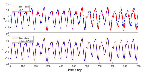
Figure 5.
Comparison of the prediction results for the MG time series between the ESN and H-ESN; the upper panel shows the ESN predictions, and the lower panel shows the H-ESN predictions.
Table 6.
Parameters for the MG time series prediction task.
As shown in Figure 5, both models can make good short-term predictions for the MG time series. The ESN can accurately predict 533 data points, but it fails to accurately predict the peak information in the time interval between 533 and 800 time steps. On the other hand, the H-ESN can predict for 1000 time steps and is capable of capturing the peak information effectively, indicating that the H-ESN has a clear advantage in predicting the MG time series.
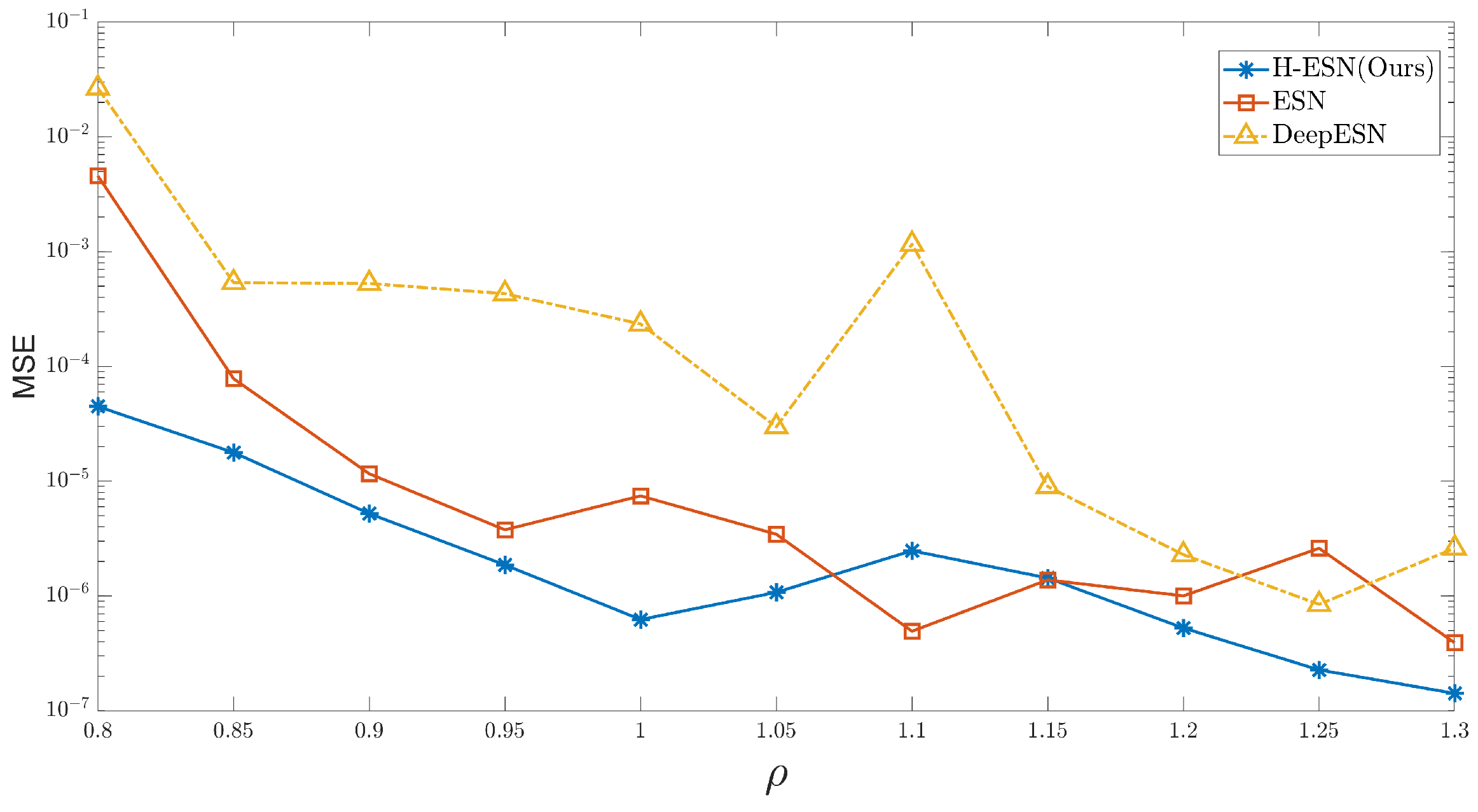
The hyperparameters in ESN have a significant impact on the prediction performance of chaotic systems. The following analysis examines how the MSE between the predicted and true values changes with the spectral radius over the first 500 time steps. Overall, as the spectral radius increases, the MSE decreases, and the H-ESN shows higher prediction accuracy compared to the other two models. For small values of , the prediction accuracy already reaches , and the MSE value reaches when = 1.3.
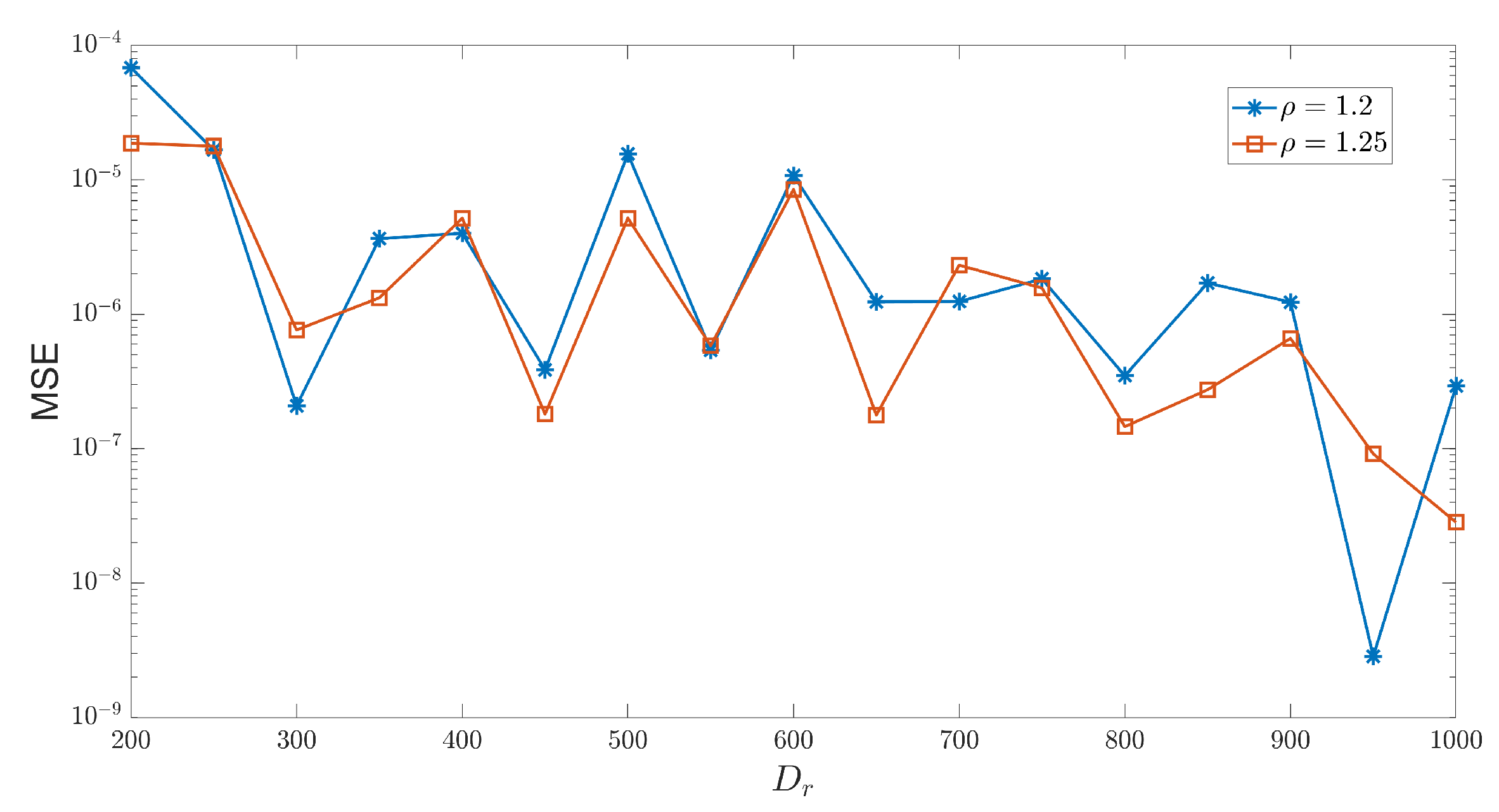
In addition to the spectral radius , which affects the prediction accuracy of the model, the number of reservoir nodes also plays a crucial role in chaotic prediction. The size of directly influences the complexity of the state space that the network can represent. Generally speaking, the larger the number of reservoir nodes, the more dynamic and complex patterns the network can capture. Figure 6 illustrates how the MSE between the predicted and true values changes with for two different spectral radii. It can be observed that when = 1.2 and = 950, the corresponding MSE is minimized, and the prediction accuracy reaches . Furthermore, Figure 6 shows that for different reservoir sizes, for = 300, the MSE corresponding to = 1.2 is smaller than that corresponding to = 1.25, which is the opposite trend compared to the one observed for H-ESN in Figure 7. This indicates that different reservoir sizes have a significant impact on the prediction ability of the H-ESN.
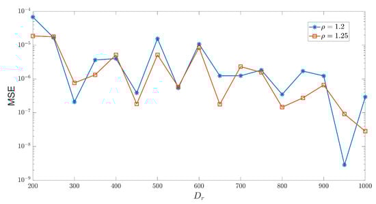
Figure 6.
Prediction error curves of the H-ESN with and as functions of varying reservoir sizes .
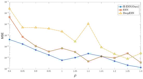
Figure 7.
Variation curves of the prediction errors of the ESN, H-ESN, and DeepESN at different spectral radius values.
3.3. Kuramoto–Sivashinsky Equations
Now consider a modified version of the Kuramoto–Sivashinsky(KS) system defined by the following partial differential Equation [43]
If , this equation is reduced to the standard KS equation, and if , the cosine term makes the equation spatially inhomogeneous. We will focus on the case where below.
We take into consideration the fact that the KS system has periodic boundary conditions at , that is, , and the KS equation is numerically integrated into a uniformly spaced grid of size Q. The simulated data consists of Q time series with time step , represented by vector , where , .
Considering that the Kuramoto–Sivashinsky equation has high dimensional spatiotemporal chaos and a certain symmetry, we modify Equation (2) by analogy with the Lorenz system. After the training stage , the system uses Tikhonov regularization regression to obtain . When the output parameters are determined, the system enters the prediction stage and independently evolves according to Figure 1b.
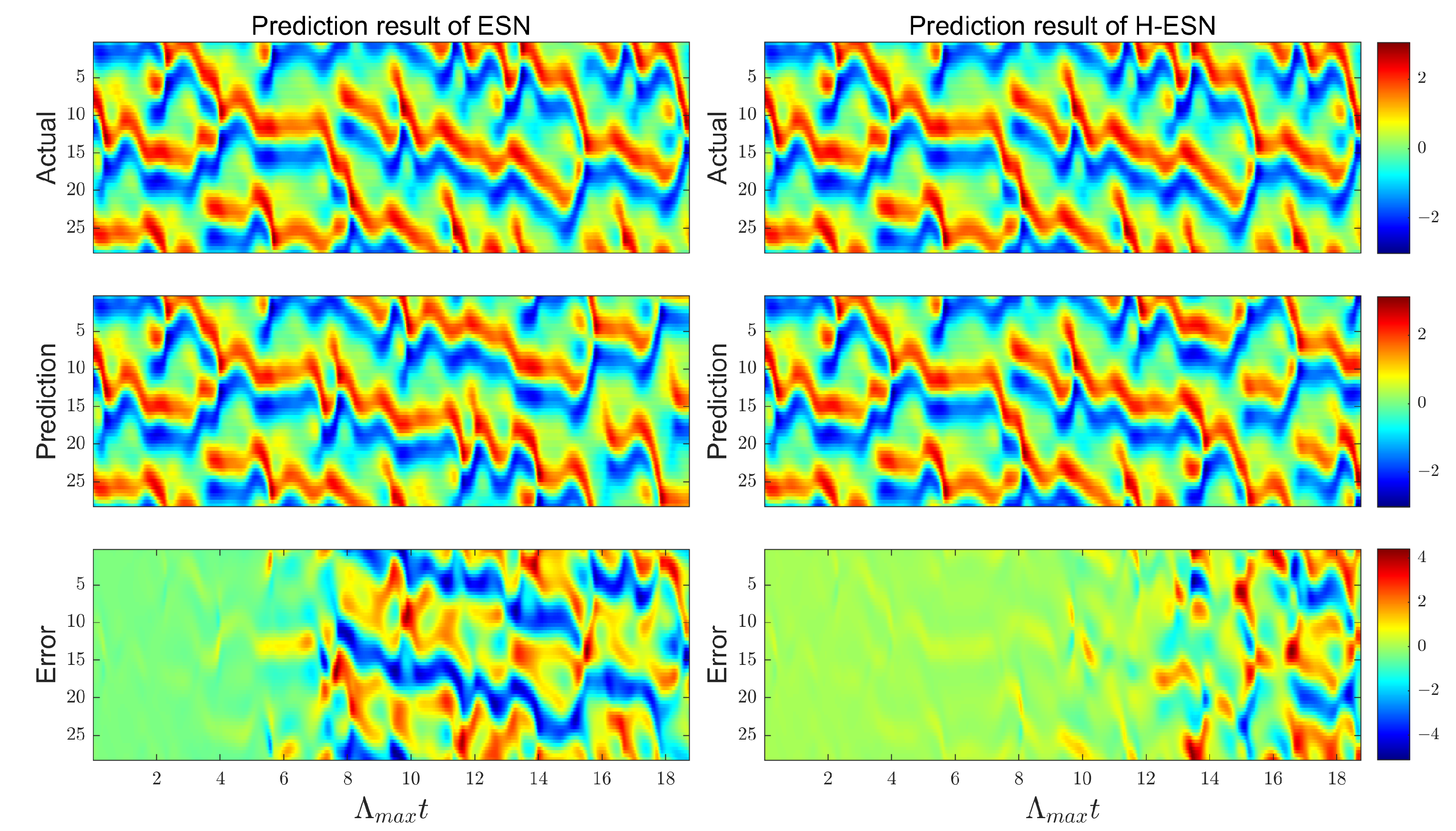
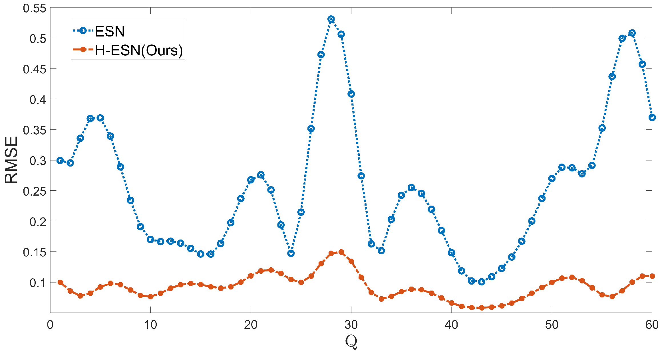
As shown in Figure 8, the ESN model achieves the prediction of 7 steps for the KS system, while the H-ESN model can predict up to 12 steps, in almost twice the duration taken by the ESN model. In terms of prediction accuracy, the error panel of the H-ESN model is close to 0 during the early prediction stages. For comparison, we have plotted the root mean square error (RMSE) of both models at different prediction dimensions Q in Figure 9. The RMSE values of the H-ESN are consistently below 0.15, with relatively small fluctuations. In contrast, the RMSE values of the ESN model are mostly above 0.15, with a significant difference between the maximum and minimum values. Therefore, the H-ESN model is more accurate in prediction and also more stable in terms of prediction performance.
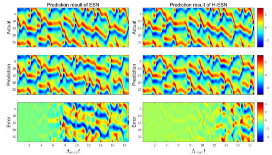
Figure 8.
Comparison of the prediction results for the KS system between the ESN and H-ESN: the left panel shows the ESN predictions, while the right panel shows the H-ESN predictions, where represents the Lyapunov time.
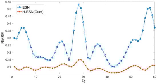
Figure 9.
MSE plot of the predicted values and true values for different dimensions of the KS system using the ESN and H-ESN.
The most important characteristic of chaotic dynamics is their extreme sensitivity to initial conditions. In chaotic systems, long-term predictions of the system’s state are impossible, as even the smallest errors will exponentially amplify, quickly eroding predictive capability. In predicting chaotic systems, not only is it necessary to optimize the hyperparameters to extend the effective prediction time of various variables, but it is also essential to evaluate the prediction accuracy in terms of the system’s inherent chaotic characteristics. The maximum Lyapunov exponent () is a key metric for measuring the chaotic nature of dynamic systems. It evaluates whether the system exhibits a chaotic behavior by quantifying the rate of divergence of nearby trajectories in the phase space. By comparing the of the KS system, as shown in Table 7, it can be observed that the estimated from the predicted data of the H-ESN model is closest to the true of the KS system, with a difference of 0.0001. In contrast, the obtained from the predicted data of the ESN model deviates from the true value by 0.0017. This difference indicates that the H-ESN model demonstrates a stronger ability to capture the chaotic characteristics and sensitivity of the system. Particularly at longer time scales, the H-ESN is able to more accurately reflect the system’s dynamical behavior, highlighting its advantages in modeling complex dynamical systems.
Table 7.
Comparison table of for the ESN and H-ESN, represents the maximum Lyapunov exponent.
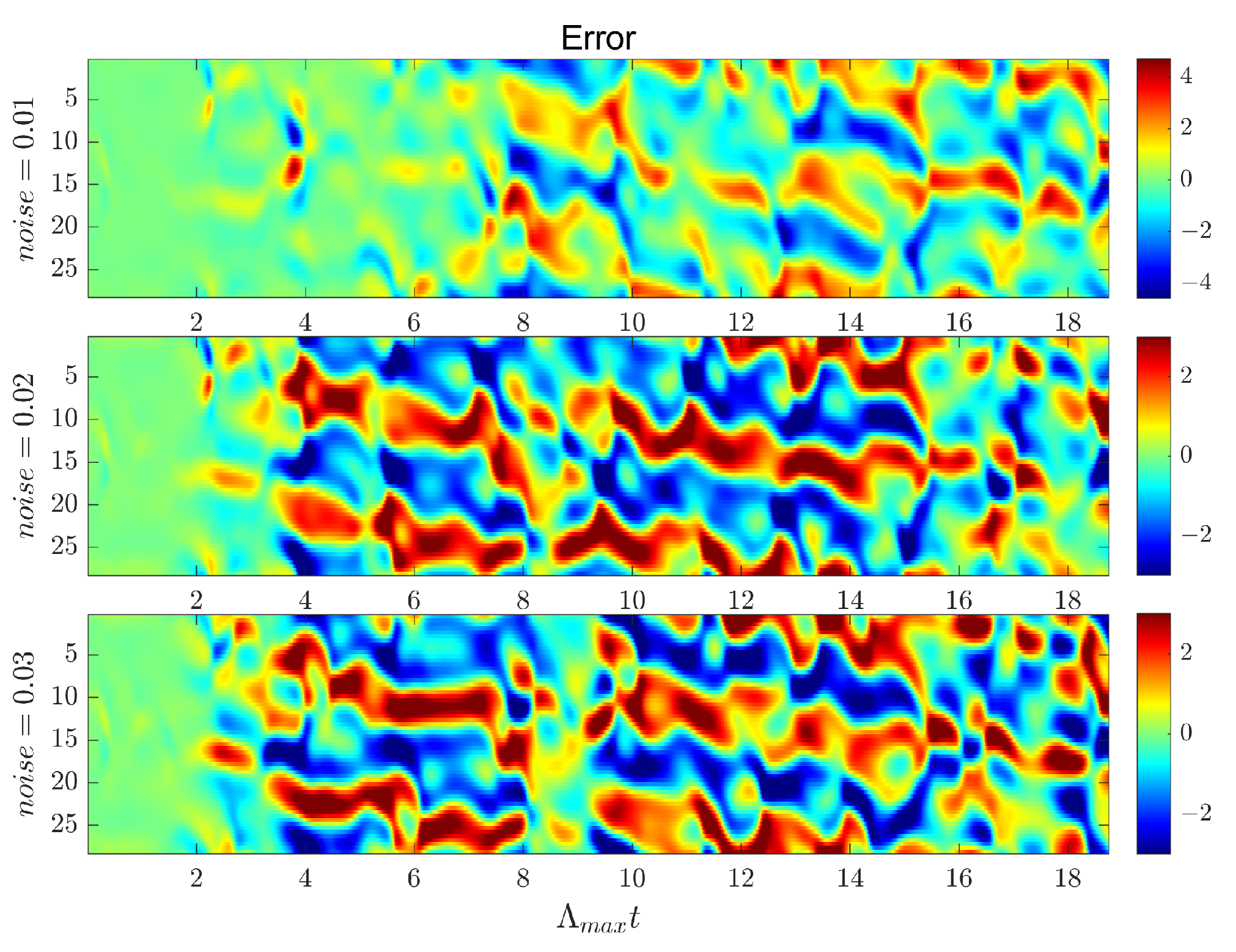
Chaotic systems are often disturbed by noise in practical applications, which can significantly reduce the performance of prediction models. To verify the robustness of the H-ESN under noisy conditions, we added Gaussian noise with varying intensities (noise levels of 0.01, 0.02, and 0.03) to the KS system, simulating real-world measurement errors. The experiment was conducted with the parameters listed in Table 8, aiming to evaluate the performance of H-ESN under noise conditions.
Table 8.
Parameters for the KS system prediction task.
As shown in Figure 10, when the Gaussian noise intensity is 0.01, the H-ESN can still maintain good predictive capability, with a prediction duration reaching 6 . However, as the noise intensity increases, the predictive capability of the H-ESN gradually declines. This indicates that in low-noise environments, the H-ESN can effectively handle noise interference and maintain high prediction accuracy; however, under high-noise conditions, the impact of noise on model performance becomes more pronounced.

Figure 10.
Comparison of prediction errors of the H-ESN under different Gaussian noise intensities.
4. Summary and Future Directions
4.1. Summary
A trained ESN can approximate the ergodic properties of its real system, and an ESN based on homotopy theory has demonstrated better performance for short-term predictions in chaotic systems. As shown in Section 3, with the Lorenz and MG system, the choice of parameters has a significant impact on prediction performance. Once the parameters are properly selected, our method has demonstrated longer prediction durations and better accuracy. For high-dimensional spatiotemporal chaotic systems, the H-ESN has demonstrated better performance in chaotic prediction compared to the ESN, doubling the prediction duration and providing more precise estimates of the Lyapunov exponent. Moreover, the H-ESN exhibits a certain degree of robustness in low-noise environments, where it retains reliable prediction capabilities even under mild noise interference. This resilience not only highlights its practical applicability but also ensures the preservation of chaotic system dynamics, making it a promising tool for real-world scenarios where complete noise elimination is challenging.
4.2. Future Directions
From a broader perspective, this paper reveals that echo state networks based on homotopy theory (H-ESN) represent a highly fruitful and detailed research direction in the field of chaotic system measurement data. However, despite its promising potential, the current H-ESN framework still exhibits certain limitations that need to be addressed.
- Computational inefficiency arises in parameter optimization, particularly in selecting the homotopy parameter .
- H-ESN exhibits certain limitations under high-noise conditions, with prediction accuracy gradually decreasing as noise intensity increases.
- Reservoir design varies by task, but the lack of universal guidelines makes selecting the right structure and parameters challenging.
Future research can focus on integrating noise reduction techniques or robust optimization methods to further enhance the performance of the H-ESN in high-noise environments. Additionally, exploring more efficient and direct approaches for selecting the homotopy parameter is crucial for improving the model’s adaptability and reducing computational costs. At the same time, developing adaptive design methods and establishing a theoretical framework can provide systematic guidance for the selection of reservoir structures and parameters in the H-ESN, thereby further enhancing its performance and generalizability across different application scenarios. These research directions not only hold significant theoretical value but also provide new insights for solving practical engineering problems.
Author Contributions
Conceptualization, S.W. and F.G.; methodology, S.W. and Y.L.; validation, S.W., F.G. and Y.L.; formal analysis, F.G. and Y.L.; investigation, H.L.; writing—original draft preparation, S.W. and F.G.; writing—review and editing, Y.L. and H.L.; visualization, S.W.; funding acquisition, Y.L. All authors have read and agreed to the published version of the manuscript.
Funding
This research was funded by the Fundamental Research Funds for the Central Universities (Grant No. 2652023054) and the 2024 Graduate Innovation Fund Project of China Universit of Geosciences, Beijing, China (Grant No. YB2024YC044).
Data Availability Statement
No new data were created or analyzed in this study.
Conflicts of Interest
The authors declare no conflicts of interest.
References
- Hinton, G.; Deng, L.; Yu, D.; Mohamed, A.; Jaitly, N. Deep neural networks for acoustic modeling in speech recognition: The shared views of four research groups. IEEE Signal Process. Mag. 2012, 29, 82–97. [Google Scholar] [CrossRef]
- LeCun, Y.; Bengio, Y.; Hinton, G. Deep learning. Nature 2015, 521, 436–444. [Google Scholar] [CrossRef]
- Silver, D.; Huang, A.; Maddison, C.J.; Guez, A.; Sifre, L.; van den Driessche, G.; Schrittwieser, J.; Antonoglou, I.; Panneershelvam, V.; Lanctot, M.; et al. Mastering the game of Go with deep neural networks and tree search. Nature 2016, 529, 484–489. [Google Scholar] [CrossRef]
- Vismaya, V.S.; Muni, S.S.; Panda, A.K.; Mondal, B. Degn-Harrison map: Dynamical and network behaviours with applications in image encryption. Chaos Solit. Fractals 2025, 192, 115987. [Google Scholar]
- Khan, A.Q.; Maqbool, A.; Alharbi, T.D. Bifurcations and chaos control in a discrete Rosenzweig-Macarthur prey-predator model. Chaos Interdiscip. J. Nonlinear Sci. 2024, 34, 033111. [Google Scholar] [CrossRef]
- Farman, M.; Jamil, K.; Xu, C.; Nisar, K.S.; Amjad, A. Fractional order forestry resource conservation model featuring chaos control and simulations for toxin activity and human-caused fire through modified ABC operator. Math. Comput. Simul. 2025, 227, 282–302. [Google Scholar] [CrossRef]
- Zhai, H.; Sands, T. Controlling chaos in Van Der Pol dynamics using signal-encoded deep learning. Mathematics 2022, 10, 453. [Google Scholar] [CrossRef]
- Kennedy, C.; Crowdis, T.; Hu, H.; Vaidyanathan, S.; Zhang, H.-K. Data-driven learning of chaotic dynamical systems using Discrete-Temporal Sobolev Networks. Neural Netw. 2024, 173, 106152. [Google Scholar] [CrossRef]
- Bradley, E.; Kantz, H. Nonlinear time-series analysis revisited. Chaos Interdiscip. J. Nonlinear Sci. 2015, 25, 097610. [Google Scholar] [CrossRef]
- Young, C.D.; Graham, M.D. Deep learning delay coordinate dynamics for chaotic attractors from partial observable data. Phys. Rev. E 2023, 107, 034215. [Google Scholar] [CrossRef]
- Datseris, G.; Parlitz, U. Delay Coordinates, in Nonlinear Dynamics: A Concise Introduction Interlaced with Code; Springer International Publishing: Cham, Switzerland, 2022; pp. 89–103. [Google Scholar]
- Brandstater, A.; Swinney, H.L. Strange attractors in weakly turbulent Couette-Taylor flow. Phys. Rev. A 1987, 35, 2207. [Google Scholar] [CrossRef] [PubMed]
- Peng, H.; Wang, W.; Chen, P.; Liu, R. DEFM: Delay-embedding-based forecast machine for time series forecasting by spatiotemporal information transformation. Chaos Interdiscip. J. Nonlinear Sci. 2024, 34, 043112. [Google Scholar] [CrossRef]
- Jaeger, H.; Haas, H. Harnessing nonlinearity: Predicting chaotic systems and saving energy in wireless communication. Science 2004, 304, 78–80. [Google Scholar] [CrossRef] [PubMed]
- Pathak, J.; Lu, Z.; Hunt, B.R.; Girvan, M.; Ott, E. Using machine learning to replicate chaotic attractors and calculate Lyapunov exponents from data. Chaos Interdiscip. J. Nonlinear Sci. 2017, 27, 121102. [Google Scholar] [CrossRef] [PubMed]
- Hart, J.D. Attractor reconstruction with reservoir computers: The effect of the reservoir’s conditional Lyapunov exponents on faithful attractor reconstruction. Chaos Interdiscip. J. Nonlinear Sci. 2024, 34, 043123. [Google Scholar] [CrossRef]
- Lu, Z.; Pathak, J.; Hunt, B.; Girvan, M.; Brockett, R.; Ott, E. Reservoir observers: Model-free inference of unmeasured variables in chaotic systems. Chaos Interdiscip. J. Nonlinear Sci. 2017, 27, 041102. [Google Scholar] [CrossRef]
- Ozturk, M.C.; Xu, D.; Principe, J.C. Analysis and design of echo state networks. Neural Comput. 2007, 19, 111–138. [Google Scholar] [CrossRef]
- Lukoševičius, M.; Jaeger, H. Reservoir computing approaches to recurrent neural network training. Comput. Sci. Rev. 2009, 3, 127–149. [Google Scholar] [CrossRef]
- Panahi, S.; Lai, Y.C. Adaptable reservoir computing: A paradigm for model-free data-driven prediction of critical transitions in nonlinear dynamical systems. Chaos Interdiscip. J. Nonlinear Sci. 2024, 34, 051501. [Google Scholar] [CrossRef]
- Köster, F.; Patel, D.; Wikner, A.; Jaurigue, L.; Lüdge, K. Data-informed reservoir computing for efficient time-series prediction. Chaos Interdiscip. J. Nonlinear Sci. 2023, 33, 073109. [Google Scholar] [CrossRef]
- Bonas, M.; Datta, A.; Wikle, C.K.; Boone, E.L.; Alamri, F.S.; Hari, B.V.; Kavila, I.; Simmons, S.J.; Jarvis, S.M.; Burr, W.S.; et al. Assessing predictability of environmental time series with statistical and machine learning models. Environmetrics 2025, 36, e2864. [Google Scholar] [CrossRef]
- Yadav, M.; Sinha, S.; Stender, M. Evolution beats random chance: Performance-dependent network evolution for enhanced computational capacity. Phys. Rev. E 2025, 111, 014320. [Google Scholar] [CrossRef] [PubMed]
- Dubey, S.R.; Singh, S.K.; Chaudhuri, B.B. Activation functions in deep learning: A comprehensive survey and benchmark. Neurocomputing 2022, 503, 92–108. [Google Scholar] [CrossRef]
- Yu, D.; Cao, F. Construction and approximation rate for feedforward neural network operators with sigmoidal functions. J. Comput. Appl. Math. 2025, 453, 116150. [Google Scholar] [CrossRef]
- Gong, Y.; Lun, S.; Li, M.; Lu, X. An echo state network model with the protein structure for time series prediction. Appl. Soft Comput. 2024, 153, 111257. [Google Scholar] [CrossRef]
- Xie, M.; Wang, Q.; Yu, S. Time series prediction of ESN based on Chebyshev mapping and strongly connected topology. Neural Process. Lett. 2024, 56, 30. [Google Scholar] [CrossRef]
- Lun, S.-X.; Yao, X.-S.; Qi, H.-Y.; Hu, H.-F. A novel model of leaky integrator echo state network for time-series prediction. Neurocomputing 2015, 159, 58–66. [Google Scholar] [CrossRef]
- Liao, Z.; Wang, Z.; Yamahara, H.; Tabata, H. Echo state network activation function based on bistable stochastic resonance. Chaos Solit. Fractals 2021, 153, 111503. [Google Scholar] [CrossRef]
- Liao, Y.; Li, H. Deep echo state network with reservoirs of multiple activation functions for time-series prediction. Sādhanā 2019, 44, 146. [Google Scholar] [CrossRef]
- Sun, C.; Song, M.; Hong, S.; Li, H. A review of designs and applications of echo state networks. arXiv 2020, arXiv:2012.02974. [Google Scholar] [CrossRef]
- Sun, J.; Li, L.; Peng, H. Sequence Prediction and Classification of Echo State Networks. Mathematics 2023, 11, 4640. [Google Scholar] [CrossRef]
- González-Zapata, A.M.; Tlelo-Cuautle, E.; Ovilla-Martinez, B.; Cruz-Vega, I.; De la Fraga, L.G. Optimizing echo state networks for enhancing large prediction horizons of chaotic time series. Mathematics 2022, 10, 3886. [Google Scholar] [CrossRef]
- Lin, Z.F.; Liang, Y.M.; Zhao, J.L.; Feng, J.; Kapitaniak, T. Control of chaotic systems through reservoir computing. Chaos Interdiscip. J. Nonlinear Sci. 2023, 33, 121101. [Google Scholar] [CrossRef]
- Li, Y.; Li, Y. Predicting chaotic time series and replicating chaotic attractors based on two novel echo state network models. Neurocomputing 2022, 491, 321–332. [Google Scholar] [CrossRef]
- Maass, W.; Natschläger, T.; Markram, H. Real-time computing without stable states: A new framework for neural computation based on perturbations. Neural Comput. 2002, 14, 2531–2560. [Google Scholar] [CrossRef]
- Faroughi, S.A.; Soltanmohammadi, R.; Datta, P.; Mahjour, S.K.; Faroughi, S. Physics-informed neural networks with periodic activation functions for solute transport in heterogeneous porous media. Mathematics 2023, 12, 63. [Google Scholar] [CrossRef]
- Arkowitz, M. Introduction to Homotopy Theory; Springer Science & Business Media: New York, NY, USA, 2011; pp. 3–7. [Google Scholar]
- Yildiz, I.B.; Jaeger, H.; Kiebel, S.J. Re-visiting the echo state property. Neural Netw. 2012, 35, 1–9. [Google Scholar] [CrossRef]
- Wang, B.; Lun, S.; Li, M.; Lu, X. Echo state network structure optimization algorithm based on correlation analysis. Appl. Soft Comput. 2024, 152, 111214. [Google Scholar] [CrossRef]
- Lorenz, E.N. Deterministic nonperiodic flow. J. Atmos. Sci. 1963, 20, 130–141. [Google Scholar] [CrossRef]
- Glass, L.; Mackey, M. Mackey-Glass equation. Scholarpedia 2010, 5, 6908. [Google Scholar] [CrossRef]
- Abadie, M.; Beck, P.; Parker, J.P.; Schneider, T.M. The topology of a chaotic attractor in the Kuramoto-Sivashinsky equation. Chaos Interdiscip. J. Nonlinear Sci. 2025, 35, 013123. [Google Scholar] [CrossRef] [PubMed]

Disclaimer/Publisher’s Note: The statements, opinions and data contained in all publications are solely those of the individual author(s) and contributor(s) and not of MDPI and/or the editor(s). MDPI and/or the editor(s) disclaim responsibility for any injury to people or property resulting from any ideas, methods, instructions or products referred to in the content. |
© 2025 by the authors. Licensee MDPI, Basel, Switzerland. This article is an open access article distributed under the terms and conditions of the Creative Commons Attribution (CC BY) license (https://creativecommons.org/licenses/by/4.0/).