Abstract
In this paper, a stochastic continuous-time Markov chain (CTMC) model is developed and analyzed to explore the dynamics of cholera. The multitype branching process is used to compute a stochastic threshold for the CTMC model. Latin hypercube sampling/partial rank correlation coefficient (LHS/PRCC) sensitivity analysis methods are implemented to derive sensitivity indices of model parameters. The results show that the natural death rate of a vector is the most sensitive parameter for controlling disease outbreaks. Numerical simulations indicate that the solutions of the CTMC stochastic model are relatively close to the solutions of the deterministic model. Numerical simulations estimate the probability of both disease extinction and outbreak. The probability of cholera extinction is high when it emerges from bacterial concentrations in non-contaminated/safe water in comparison to when it emerges from all infected groups. Thus, any intervention that focuses on reducing the number of infections at the beginning of a cholera outbreak is essential for reducing its transmission.
Keywords:
infectious disease; Latin hypercube sampling; multitype branching process; partial rank correlation coefficients; stochastic model; stochastic threshold MSC:
35R60; 60J28; 60J80; 92B05
1. Introduction
Infectious diseases have a tremendous impact on human health. Thus, it is essential to research the mechanisms of disease transmission and the control of diseases like cholera. Controlling an infection and protecting human health require an understanding of the dynamic nature of infectious illnesses [1]. Food-borne diarrheal illness, or cholera, is one of the most serious infectious diseases [2]. Vectors, also known as carriers, include things like house flies, ticks, mites, etc., which are also a means for food-borne diseases. Even though cholera is mostly a waterborne disease, fly vectors can indirectly spread it [3]. Fly-carried cholera-causing bacteria are introduced into the food supply and contaminate human meals [4,5]. Eating this tainted food exposes susceptible populations to cholera infection [6]. House flies eat on, crawl over, and deposit their eggs on human food, which is how they transmit cholera to humans [7]. One public health concern the WHO has recognized is cholera [8]. The literature contains numerous investigations of theoretical and clinical studies. Despite documentation [9], the public health of developing countries is still seriously endangered by cholera. The need to model cholera transmission is still crucial, despite the fact that cholera has been studied extensively and despite prevention measures being well established. Cholera still causes recurrent outbreaks, especially in low-resource settings because of the effects of climate change (e.g., floods and droughts increasing transmission risks), conflict and displacement (e.g., poorly sanitary refugee camps), and urbanization and population growth (e.g., water and sanitation challenges) [10,11,12].
In epidemiology, mathematical modeling is essential for understanding and predicting disease outbreaks [13]. A useful technique for understanding the transmission of diseases is mathematical modeling, which may be used to predict future epidemics and provide strategies for managing epidemics [14,15]. A disease’s epidemiological model may be stochastic or deterministic. In the modeling of diseases, both kinds of models are helpful. Deterministic models are mostly used because of their simple formulation and analysis of a system of ordinary differential equations compared to stochastic models [16]. Deterministic models can be used to predict whether or not a disease would spread based on the value of the fundamental reproduction number. Deterministic models, on the other hand, are unable to adequately represent the uncertainty and variability that real-life epidemics entail because of environmental factors or demographic shifts, which is important when the initial number of infected individuals is small [17]. Specifically, when an infectious individual is introduced into an entirely susceptible community, there is a chance they may either die or recover before infecting a substantial number of susceptible individuals [18,19]. For sufficiently small populations, deterministic models are more challenging to estimate and analyze, and they provide less information. In addition, trajectories in deterministic models deviate from expected noise behavior due to random influences [20]. Owing to those drawbacks, stochastic modeling of infectious diseases in both homogeneous and heterogeneous populations arose as a substitute for deterministic models, mitigating some of the issues associated with deterministic models when modeling epidemic diseases [21]. Stochastic models are capable of handling randomness and thus can produce distinct results for each input that is supplied. In deterministic models, an identical output is produced for each input since they are unable to handle randomness [22]. Despite their benefits and potential usefulness for systems with causal relationships and clearly stated rules, deterministic models frequently fail to capture the unpredictability, uncertainty, and intricacy present in numerous real-world systems. Because they offer a more adaptable and realistic method of simulating such intricacy, stochastic systems are a valuable tool in many scientific and engineering applications [23,24]. Stochastic models are preferred because disease transmission in real life is highly random, even though deterministic models are mathematically easier to analyze. A stochastic model is required for our study to capture cholera’s real-world variability and predict both extinction and outbreak probabilities. Thus, it is crucial to take into account a stochastic model in order to reflect the variability related to individual dynamics (such as birth or death, transmission, and recovery), also known as demographic variability [25]. The transmission of cholera through fly vectors is largely random because of a number of circumstances, such as fly vectors’ contribution to Vibro cholera in the environment, parasite acquisition, human immune responses, and the effectiveness of treatments. The continuous-time Markov chain (CTMC) stochastic model incorporates random events, which makes it feasible to mimic these stochastic processes and represent the variability seen in actual cholera dynamics. Cholera infection progression via fly vector transmission involves discrete states of human, vector, and bacterial (pathogenic) populations [26]. It is acceptable to use CTMC stochastic models to observe the dynamics of cholera infection over time because they are useful for representing such distinct states and the transition between them. Additionally, individual-level heterogeneity can be incorporated into the CTMC stochastic model, allowing us to carry out host population simulations and capture the impact of heterogeneity on disease transmission and outcomes [27]. With respect to the particular biological processes involved in cholera dynamics, CTMC stochastic models use transition rates between states, which establish the likelihood of changing states. However, the CTMC stochastic model can depict time-dependent events, such as the arrival of the infected fly vector, the growth of the parasite, and the recovery processes. The stochastic and continuous evolution of disease states over time can thus be described [27]. Cholera’s complexity, stochasticity, and temporal dynamics are thus captured by the CTMC stochastic models, making them appropriate for cholera research. Cholera transmission and infection dynamics are more realistically represented using the CTMC stochastic model, which facilitates the simulation of discrete infection states, time-dependent events, and individual-level variations. The value of the current state at time t determines the transition of any state variable to the state i at time t, according to the Markov property, not the filtration or process history. In the CTMC stochastic model, time is considered to be continuous, the state variables are discrete-valued, and the process is time-homogeneous with the Markov property [27].
In relation to the idea of ODE epidemiological dynamics, [25] developed the notion of stochastic epidemic modeling. Her prominence was especially notable in stochastic differential equations and continuous-time Markov chains. Stochastic thresholds depend on the size of the population and the likelihood of disease extinction within each of the multiple infectious subgroups [28]. The likelihood of a major disease outbreak for a single group of infections is around , where denotes the basic reproduction number and i represents infectious individuals. A vector-borne disease’s activity might be influenced by a specific time of year or seasonal change. As a result, seasonal fluctuation and the initial population infection rate influence the likelihood of a disease outbreak, which may occur periodically [29,30]. When the population is big enough and the basic reproduction number is greater than one, the probabilities of a disease outbreak estimated from stochastic CTMC models and branching process approximation coincide [31]. When modeling epidemics, the CTMC model is preferable to deterministic models and the measured trajectories follow expectations [32]. If both the host and vector populations are smaller than 100, the branching process approximation might not produce a reliable estimate [29,31]. The detail of branching process approximation is introduced in Section 3.1 of this paper. Several studies have been conducted to study the spread of cholera in deterministic and stochastic model settings [21,33,34,35,36]. The stochastic CTMC model, with varying parameter values, and the starting number of infected persons for cholera are used to approximate the probability of an outbreak [33]. In the study of [36], a stochastic population represented by a set of stochastic differential equations (SDEs) was used to investigate the dynamics of cholera transmission. They examined how disease dynamics behaved in deterministic and stochastic randomness-based models. They stated that the stochastic perturbation is demonstrated to improve the stability of the disease-free equilibrium when compared to the underlying deterministic model due to the fact that stochastic extinction of the disease is an absorbing state. The authors of [21] analyzed the SDEs’ cholera model, and they found that the stochastic solution fluctuates around the solution of the ordinary differential equation model. The stochastic model of cholera has been used in other studies [34,35] to simulate the population of bacteria in contaminated water and human contact with the bacteria in the water supply. These studies focus on how the disease spreads. However, none of the stochastic studies have considered the impact of fly vectors in the transmission dynamics of cholera. Human and fly vector heterogeneity can have a significant impact on the dynamics of cholera transmission. For instance, the rate of contribution to Vibrio cholera in the environments by fly vectors, human immunity, and treatment-seeking behaviors varies among individuals and populations. The fly vectors’ contribution to Vibrio cholera is stochastic with the frequency of contaminating human meals and infectivity rates. Individual variations have also been noted in the dynamics of immunity development, parasite proliferation, and immune responses [37,38]. Furthermore, interventions such as treatment plans (such as medication delivery and case supervision) provide other sources of randomness and variability. A stochastic model helps to investigate the biological complexity and variability of cholera dynamics. It also provides a more accurate depiction of the behaviors of transmission, the outcomes of infections, and the impact of interventions. The stochastic model contributes to a better understanding of cholera epidemiology, prevention strategies, and the possible outcomes of treatments in different scenarios by examining the probabilistic nature of the disease. Thus, a stochastic model is well justified in studying cholera transmission dynamics due to the biological foundations. No study has applied a stochastic CTMC model to study the dynamics of cholera via fly vector transmission to the best of the knowledge the authors so far. In this study, we formulate and analyze a stochastic CTMC model by extending the deterministic model developed in [26] and apply the theory of the multitype branching process to determine the probability of cholera extinction or outbreak.
The article is organized as follows: In Section 2, a deterministic cholera epidemic model formulated by [26] is presented. In Section 3, the corresponding stochastic CTMC model of cholera is formulated with the multitype branching process in Section 3.1 and stochastic threshold in Section 3.2. Section 4 is devoted to the sensitivity analysis using Latin hypercube sampling (LHS) and partial rank correlation coefficient (PRCC) procedures. In Section 5, the results are presented, and their interpretation is examined. A brief discussion of the findings is given in Section 6. Lastly, Section 7 provides a final summary of the findings.
2. Model Formulation
This section introduces a deterministic cholera model formulated by [26]. In their model, the human or host population is subdivided into four compartments, depending on the epidemiological status of individuals, namely , which denotes the number of susceptible individuals; , which denotes symptomatic infected individuals; , which denotes asymptomatic infected individuals; and , which denotes recovered individuals at any given time t. Similarly, the vector population is subdivided into three compartments—susceptible vectors , exposed vectors , and infected vectors —at any given time t. Bacterial concentrations in contaminated/unsafe water and bacterial concentrations in non-contaminated/safe water are the bacterial (pathogenic) population at any given time t. The parameters used in the model formulation are summarized in Table 1. From the description of the dynamics of cholera, as shown in Figure 1, we have the following system of non-linear differential equations [26]:

Table 1.
Parameters and their descriptions of the model.
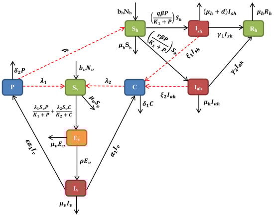
Figure 1.
Model flowchart showing the compartments.
Reproduction Number
In epidemiology, the basic reproduction number, or , is an important parameter. It is also known as the basic reproductive rate or basic reproductive ratio. A single primary infectious case introduced into a whole susceptible population that is known to transmit an average number of secondary infectious cases is referred to as a basic reproduction number [39]. This parameter is useful for predicting the likelihood of an infectious disease spreading across the population or not. To compute , the next generation matrix approach is applied, as described in [40]. To obtain it, take the largest (dominant) eigenvalue value (spectral radius) of
where is the rate of appearance of a new infection in compartment i, is the net transition between compartments, is the disease-free equilibrium and stands for the terms in which the infection is in progression, i.e., , and P in Equation (1). Hence, the basic reproduction number obtained in [26] was as follows: where quantities and are contributions of the human and vector/housefly infectious classes, respectively.
3. Formulation of Continuous-Time Markov Chain (CTMC) Model
Numbers used in these stochastic models are integers rather than constantly changing values because models with demographic variability reflect a discrete shift of individuals within epidemiological classes rather than an average rate [18]. A stochastic CTMC cholera model is thus developed in this study according to the assumptions of the deterministic cholera model Equation (1), as time is continuous and the variables that are random equivalent to the deterministic state variables are discrete. For convenience, we use the same notation for the variables that are random and parameters in Equation (1) for the deterministic model. Let , and denote discrete random variables for the number of individuals in the susceptible, symptomatic, asymptomatic, and recovered host population classes, and let , and denote discrete random variables for the number of susceptible, exposed, and infected vector population classes at , respectively. Also, in the cholera deterministic model (Equation (1)), there are and , which denote the concentration of Vibrio cholerae in the contaminated/unsafe water and non-contaminated/safe water at time t, respectively. However, and are not compartment occupancies as the other ones, so their transition here is not considered in the formulation of transitions [33]. Here, the variables , and take values in the finite state space {0, 1, 2, 3, …, G}, where G is the greatest size of the entire population. According to the CTMC model, a state transition can happen at any time t. All potential state transitions for the CTMC model are shown, along with the rates at which they occur in Table 2.
Table 2.
Stochastic continuous-time Markov chain (CTMC) model rate of changes.
The continuous-time stochastic process is a process that has multiple variables and a joint probability function [41,42]
which is homogenous in time and meets the Markov property, which states that the process’s future state at time depends only on the present state of the process at time t [18,41]. Hence,
The Markov assumption states that the time until the next occurrence is exponentially dispersed [18,41]. Depending on the notation used in [41], we obtain the stochastic process’s infinitesimal transition probabilities from state at time t to a new state at time as follows:
which are defined by
where
Applying the Markov property to the stochastic process and the infinitesimal transition probabilities given above, we can express the state probabilities at time in terms of the state probabilities at time t [43]. Thus, the state probabilities satisfy the following difference equation:
To investigate the time evolution of , we adjust the parameters of Equation (3). Then we take the limit as . Following that, the forward Kolmogorov differential equation is obtained as follows:
3.1. The Multitype Branching Process
The multitype branching process approximation is a powerful tool that provides additional insights into the probability of reaching the disease-free equilibrium, especially in early outbreak dynamics and near-extinction scenarios. The multitype branching process is solely implemented to the infected groups in order to assess the dynamics of the non-linear CTMC model, and it assumes that susceptible individuals are in the disease-free equilibrium [18,28,44]. It is useful in computing the probabilities of disease extinction or outbreak. In CTMC models, if there are a few infectious agents present at the start of the disease outbreak, there is a chance that the disease will either die or spread [25]. The initial susceptible population must be sufficiently large at disease-free equilibrium for the multitype branching process to occur. Thus, in this paper, we use and [45]. The multitype branching process is homogenous in time and independent of births (i.e., new infections) and deaths or recovery, since it is linearly close to the disease-free equilibrium. Therefore, it would be possible to describe the offspring-probability-generating functions for the birth and death of infected individuals. The likelihood of a significant breakout or the extinction of a disease is then estimated using these probability-generating functions [18,44]. The following assumptions underlie the multitype branching process approximation used to compute the stochastic threshold for the CTMC model [25]:
- The behavior of each infectious individual is independent from that of other infectious individuals.
- Both the probability of recovery and the probability of transmitting an infection are the same for each infectious individual.
- The susceptible population is sufficiently large.
Let be the offspring random variables for type { 0, 1, 2, 3, …, n}, so that is the number of offspring of type j generated by infectious individuals of type i. The offspring-probability-generating function for infectious population is defined if there is initially one infectious individual at the beginning of the disease outbreak, e.g., , and all other types are zero, . The offspring pgf for type i individuals given and is given as [19,45]:
where
is the probability that one infected individual of type i gives birth to individuals of type j [18]. Equation (5) is used to find a non-negative and irreducible expectation matrix , where is the expected number of offsprings for individuals of type j produced by an infective of type i. The elements of matrix are obtained by differentiating with respect to and then evaluating all the x variables at 1 [19,46], as follows:
The probability of disease extinction or an outbreak is determined by the size of the spectral radius of the expectation matrix , . If , then the probability of disease extinction is one, as follows:
and if , then there exists a positive probability such that the disease persists in host and vector populations, as follows:
where is the offspring pgf’s unique fixed point, and , [18,46]. For type i infectives, the value of represents the probability of disease extinction, and the probability of an outbreak is [18,19]
3.2. Stochastic Threshold for CTMC Model
In the CTMC stochastic model, the multitype branching process is applied to each infectious class in order to formulate their probability-generating functions. The branching process, which is a birth and death process for , , , , , and , can produce secondary infections. Therefore, the variable will not be considered in the branching process approximation. The bacterial concentrations in non-contaminated/safe water (P(t)) are considered since the fly vector obtains an infection from contaminated/unsafe environments and transmits to it after the susceptible population will become infected from it [26]. Accordingly, in a stochastic CTMC cholera model, an outbreak may not still die out due to chance, especially when initial bacterial concentrations are high. The initial values for susceptible individuals and susceptible vectors are considered to be the disease-free state points and , respectively. The offspring-probability-generating functions (pgfs) for infectious classes are obtained by applying the formula in Equation (5), evaluated at disease-free equilibrium. Thus, the offspring-probability-generating function for , given that , , , , and , is
The term represents the probability that a Vibrio cholera bacterium is shed by a symptomatic infected individual into the environment, while the term is the probability that the symptomatic infected human can perish or recover before infecting other susceptible individuals, thus resulting in zero infected humans.
The offspring-probability-generating function for , given that , , , , and , is
The term describes the probability that a Vibrio cholera bacterium is shed by an asymptomatic infected individual into the contaminated environment. The term is the probability that an asymptomatic infected human can perish or recover before infecting other susceptible individuals, thus resulting in zero infected humans.
The offspring-probability-generating function for , given that , , , , and , is
The term represents the probability that a latently infected vector would successfully spread the infection during their lifetime. The term stands for the probability that a latently infected vector would die before becoming infectious, leaving zero latently infected and infectious vectors.
The offspring-probability-generating function for , given that , , , , and , is
The term denotes the probability that a Vibrio cholerae bacterium is directed by the infected vector into the contaminated environment, while the term is the probability modified by the parameter that a Vibrio cholera bacterium is directed by the infected vector into the safe environment, resulting in susceptible individuals that are successfully infected after consumption. The term is the probability that the diseased vector will die before infecting a vulnerable individual, leaving no infectious individual.
The offspring-probability-generating function for C, given that , , , , and , is
where . The term is the probability that the Vibrio cholera bacterium from the contaminated water creates a latently infected vector. The term is the probability that the vibrios of the contaminated water die.
Similarly, the offspring-probability-generating function for P, given that , , , , and , is
where . The term is the probability that the Vibrio cholera bacterium from safe water creates a latently infected vector. The term is the probability that the vibrios in pure water die.
Using Equation (6), the expectation matrix of the offspring PGFs computed at is given by
The stochastic threshold for cholera disease extinction or outbreak for the CTMC epidemic model is the spectral radius of the expectation matrix, . The thresholds for the stochastic model and the basic reproduction number for the deterministic model are closely related [18]. Cholera dies if or . In deterministic models, cholera persists if . However, in stochastic models, if , there is a possibility for cholera to die or persist, depending on the number of infectives at the beginning of disease outbreak [19,44]. Thus, if , there exist a fixed point of the offspring-generating functions (10)–(15) that is used when writing the probability of cholera extinction [18,28]. To obtain the fixed point, we set for to obtain the following system of equations:
Generally, due to the non-linearity of probability-generating functions, it is not easy to obtain simple analytical expressions for the fixed points , and of the system of Equation (16) [46]. However, there are some special cases that can be considered when trying to obtain these expressions. If , we obtain
Therefore, given the initial numbers of , and , the probability of extinction for cholera is approximated to be [25,28]
Furthermore, the probability of an outbreak or disease persistence will be estimated by
4. Monte Carlo Sampling Technique (Sensitivity Analysis)
Monte Carlo sampling methods, commonly known as the LHS scheme, offer the advantage of sampling parameters independently of one another [47]. Studies have mathematically shown that LHS reduces variance in sensitivity measures and is more efficient with fewer samples [48,49,50]. LHS biases and limitations can be successfully minimized by using efficient sampling approaches, controlling correlations, ensuring sufficient coverage, and confirming results with robustness checks. These strategies improve the sensitivity analysis’s reliability to accurately capture the full range of variability in model parameters [51]. LHS/PRCC sensitivity analysis is a useful technique that is frequently used in uncertainty analysis in order to explore the entire parameter space of a deterministic or stochastic mathematical model with a minimum number of computer simulations [52]. It also measures the degree of linear relationship between inputs and outputs in order to provide PRCC indices, as per the methodology outlined by [53]. The LHS/PRCC sensitivity analysis method explores the multi-dimensional parameter space globally to identify important parameters whose uncertainties contribute to the imprecision of the prediction. In order to ascertain the degree of uncertainty that the LHS parameter adds to the prototype, the partial rank correlation analysis provides a PRCC and proportional p-values [54]. The parameter’s contribution to model predictions appears to be imprecise, based on both its magnitude and statistical significance of the PRCC value. Time-varying sensitivity for PRCC helps to determine if the significance of one parameter is noticeable over an entire time interval during model dynamics. The output measure in this case is positively correlated with a positive PRCC value, while the output measure and a negative PRCC value are inversely correlated. PRCC values (>0.5 or <−0.5) and corresponding small p-values (<0.05) are found for the most significant parameters. The closer the PRCC value is to or , the more of an impact the LHS parameter has on the outcome measure. PRCC indices that are near to or equal to zero have no significance in the context of statistical inference. A positive PRCC value indicates that an increase in a model’s parameter leads to an increase in disease persistence, whereas a negative PRCC value indicates that an increase in a model’s parameter leads to a higher likelihood of disease extinction. In particular, disease persistence is significantly influenced by high positive PRCC values of model parameters, whereas disease extinction may result from high negative PRCC values of model parameters. The variable in Equation (1) is used to demonstrate the change in PRCC indices with time. The maximum and minimum values are mandated for each of the fifteen LHS parameters in Table 3 using baseline parameter values from Table 6, which depend on our considered model. Note that the baseline value for each LHS parameter was assigned to a value that is in the middle of the range between the parameter’s minimum and maximum values.
Table 3.
Baseline, minimum, and maximum values used in the LHS analysis.
In this section, we have conducted a sensitivity analysis to ascertain the robustness of Equation (1) to parameter values to find the most significant parameters in the model dynamics. The LHS scheme, also referred to as Monte Carlo sampling, makes use of a uniform distribution to sample 1000 values for each input parameter within the range of biologically realistic values described in Table 3. For the system of differential equations described in Equation (1), 5000 model simulations were carried out by randomly selecting paired sampled values for each LHS parameter. The impact of each parameter versus the selected variables and associated uncertainties on the system of Equation (1) was elucidated by the LHS/PRCC analysis results. The LHS/PRCC analysis of and is not taken into account because they are not compartment occupants like the others [33]. Figure 2 and Figure 3 show the corresponding non-linear but unmodulated relation between model state variables and each parameter of the PRCCs and corresponding p-values. Moreover, the output is statistically significant if the corresponding p-value is less than 1%.
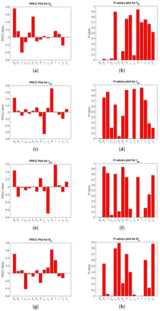
Figure 2.
PRCC and p-values’ plot for the host population.
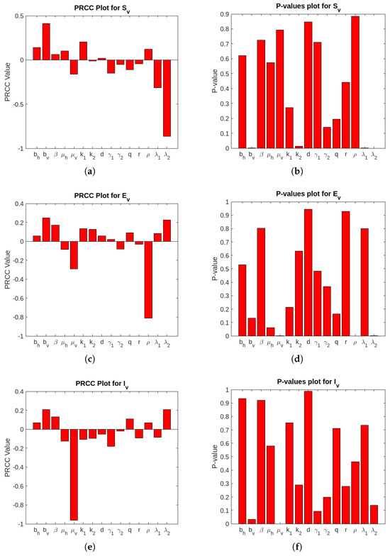
Figure 3.
PRCC and p-values’ plot for the vector population.
Figure 2 and Figure 3 visually represent the PRCC indices, highlighting that (natural vector death rate), (rates of ingesting vibrios from the contaminated/unsafe environment to vector), and (infectious rate of a vector) on outputs have strong inverse relationship. Conversely, parameters like (birth or recruitment rate by human) and (concentration of the bacteria, i.e., Vibrio cholerae in pure/safe water) demonstrate the direct relationship with the model outputs. These findings suggest the important variables to be considered for effective control strategies. We perform a multilinear regression analysis of the ranks attained to examine the regression coefficients for the consequence measures (i.e., total infected vectors ()) and the LHS parameters. PRCC values are gathered in order to determine the degree of correlation between the LHS parameter and each consequence measure, as these regression coefficients demonstrate the model’s sensitivity to the LHS parameters. Figure A1 in Appendix A shows the PRCC plots for infected vectors. The plots include the PRCC value and p-value for total infected vectors. The residuals for the ranked LHS parameter values are plotted on the y-axis in Figure A1. We have also plotted the residuals for the ranked total infected vectors on the x-axis of Figure A1. Furthermore, take note of the correlation between different LHS factors, as shown by the PRCC graph for the shown consequence measure.
Analysis of the PRCC Results
The PRCC diagram results are summarized in Table 4 and Table 5. The p-values (orange) and PRCC values (blue) of the significant uncertainty factors are both highlighted in these tables. Here, (*) is used to indicate potential contributions (PRCC values: [0.5 to 0.6) or [−0.5 to −0.6), (**) is employed to determine the most likely sources of ambiguity (PRCC values: [0.6 to 0.8) or [−0.6 to −0.8), and (***) is employed to identify the most likely sources of uncertainty (PRCC values: [0.8 to 1) or [−0.8 to −1)). From Table 4 and Table 5, we note that the most significant LHS parameters for the consequence measure are (death rate of the vector), (rates of ingesting vibrios from the contaminated/unsafe environment to vector), and (infectious rate of a vector).
Table 4.
PRCC output for host population.
Table 5.
PRCC output for vector population.
From Table 4 and Table 5, it is also evident that the PRCC values of are higher than those of the other parameters. It is concluded that is the most prominent parameter in the considered model. A higher value of reduces the environmental load of the pathogen and, consequently, secondary infections, whereas a low value allows for prolonged bacterial survival, increasing the likelihood of exposure and reinfection. may be a robust and effective cholera control strategy in urban areas with poor sanitation where environmental contamination is widespread and cholera transmission dominates.
5. Numerical Simulations
The Gillespie algorithm, which was proposed by [55], is used to simulate the sample path of the stochastic CTMC model formulated in this study. It simulates each transition event sequentially but requires a significant amount of computation time. To study the dynamics of cholera via vector transmission, both deterministic and CTMC stochastic models are plotted on the same graphs, using parameter values in Table 6 for comparison purposes for the state variables symptomatic infected hosts, asymptomatic infected hosts, and infected vectors. The graphical solutions of the CTMC model with their corresponding deterministic solutions are shown in Figure 4. The findings’ figures show that CTMC model results for the dynamics of cholera are relatively close to deterministic model solutions. The CTMC model solutions fluctuate around the solutions of the corresponding deterministic model. This further suggests that the deterministic model’s dynamical behaviors would not be impacted by the initial condition, but the CTMC model’s behaviors would be heavily reliant on it. In Figure 4d,e, the symptomatic infected host (red curve) and infected vector (blue curve) as well as asymptomatic infected host (pink curve) and infected vector (blue curve) are drawn. After a certain period, it can be seen in the figure that the symptomatic infected host, asymptomatic infected host, and infected vector curve hit the x-axis. Thus, the symptomatic infected host, asymptomatic infected host, and infected vector vanish gradually.
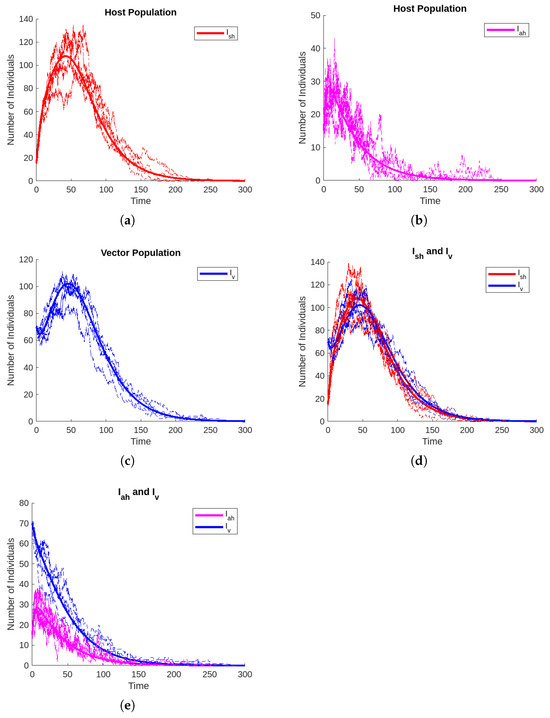
Figure 4.
Solutions for the CTMC model and the associated deterministic model that exhibit dynamic behaviors. The CTMC model solutions under five randomly chosen sample paths are shown by the solid color curves, while the deterministic model solutions are represented by the matching solid lines.
Probability of Cholera Disease Extinction or Outbreak
We determine the probability of disease extinction under various initial conditions. The initial size of the infectives determines the dynamics of cholera, as shown in Table 7. Thus, even though the stochastic threshold , cholera may vanish or persist. As shown in Table 7, the probability of cholera disease extinction is the largest when , the probability of disease prevalence , is the lowest. Furthermore, is smaller if the disease is introduced by . In particular, when the number of all six infected groups increases, the likelihood of disease extinction decreases . In other words, the probability of a disease outbreak is very high if all six infected groups are present at the onset of the epidemic process. The probability of a disease outbreak is very high if cholera emerges from all infected classes, and the situation worsens if the number of infectives increases, as shown in Table 7. The bacterial concentrations in contaminated/unsafe water play an important role because they infect a massive number of housefly vectors in the environment [3,4,5]. Thus, it is suggested that any interventions that focus on reducing the number of infected groups at the beginning of an outbreak are essential for reducing the transmission of cholera.
Table 7.
Probabilities of disease extinction and outbreak of the disease.
Table 6.
Parameter values.
Table 6.
Parameter values.
| Parameter | Base Line Value | Reference |
|---|---|---|
| 10 day−1 | [56] | |
| 1.066 day−1 | Assumed | |
| 0.005 year−1 | [57] | |
| 0.189 day−1 | [58] | |
| 0.2143 day−1 | [59] | |
| 500 cells/day | Assumed | |
| 500 cells/day | [57] | |
| 20 cell/ml per day | [60] | |
| 20 cell/ml per day | Assumed | |
| 12 cells mL−1 d−1 per vector | [61] | |
| 0.4 | Assumed | |
| d | 0.015 | [56] |
| 0.14 per day | [62] | |
| 0.5 per day | [62] | |
| q | 0.7 | [63] |
| r | 0.3 | [63] |
| 0.8 | Assumed | |
| 0.1 | Assumed | |
| 0.9 | Assumed | |
| 0.4 day−1 | [64] | |
| 0.4 day−1 | Assumed |
6. Discussion
In this paper, a stochastic CTMC model was developed, accounting for the demographic diversity that emerges in the dynamics of cholera transmission (including changes related to population dynamics, including births, infections, deaths, recovery, and relapses, among others). The integration of Monte Carlo sampling, LHS/PRCC sensitivity analysis, and deterministic model comparisons in our formulated model ensured the robustness of the numerical simulations in estimating the probability of cholera extinction under varying initial conditions and intervention scenarios. The probability of disease extinction and outbreaks, as well as the model’s stochastic threshold , were determined by the use of multitype branching processes. In general, when and , the disease would become extinct for both the stochastic and deterministic models. For the stochastic model, disease extinction is possible if . On the other hand, for the deterministic model, the disease would persistent if . We used numerical simulations to validate our analytical findings and represent them graphically in the CTMC stochastic model. We also obtained the likelihood of disease extinction or an outbreak under various initial conditions. It is clear that an acceptable agreement is found between the dynamical behavior of the deterministic and CTMC stochastic models. Our results in Figure 4 show that the CTMC model’s results for the dynamics of cholera are comparatively close to deterministic model solutions. The solutions of the CTMC model show fluctuations in the solutions of the corresponding deterministic model. As one of the primary asymptotic differences between deterministic and stochastic models, the intrinsic demographic stochasticity of stochastic models may be the cause of this discrepancy, which suggests that the dynamical behaviors of the CTMC model would be strongly influenced by the initial conditions [25,65]. Integrating LHS/PRCC sensitivity analysis with the stochastic CTMC model simulations for cholera transmission dynamics is powerful but also challenging due to the discrepancy between deterministic sensitivity and stochastic behavior. Apart from showing behavior that is essentially the same to that of the deterministic model, the stochastic CTMC model also has a positive probability association to disease extinction, regardless of the value of . However, if , disease extinction takes an exceedingly long time [17]. It is further shown that after a certain period of time, the number of infected hosts and vectors steadily declines. Thus, the strategy’s efficacy in minimizing and progressively preventing disease outbreaks is guaranteed by our preferred model. This study can be further extended in the future by examining the cross transmission of fly vectors. Another area of research word investigating could encompass the impacts of environmental and seasonal variability on disease transmission trajectories, such as seasonal rainfall, air temperature, moisture levels, and the other climatic factors that may affect the transmission dynamics of cholera. Hence, it is important to develop a stochastic CTMC model in order to investigate the effects of seasonal variation on cholera transmission dynamics [29]. The integration of stochastic CTMC, climate variability, and adaptive interventions is crucial for improving cholera extinction and persistence predictions. Future cholera modeling studies should also focus on developing a model that incorporate spatial transmission dynamics to capture regional heterogeneity, real-time adaptive models to inform public health interventions more effectively, and leverage machine learning and Bayesian methods for improved parameter estimation and outbreak forecasting.
7. Conclusions
In this study, a stochastic CTMC model was formulated and analyzed to gain insights into the transmission dynamics of cholera. We considered a sensitivity analysis for each parameter of the model. Beyond focusing on reducing initial infectives, (natural vector death rate), (rates of ingesting vibrios from the contaminated/unsafe environment to a vector), (infectious rate of a vector), and (birth or recruitment rate by a human) are important parameters that should be considered for effective cholera control strategies. The multitype branching process was adopted to derive the corresponding stochastic threshold for the CTMC model, which determines the condition for the extinction or outbreak of cholera. Generally, cholera vanishes if and . However, if , then there is a chance of a major disease outbreak or extinction depending on the initial number of infectives at the beginning of the disease outbreak. On the other hand, if , cholera persists. We established theoretical results and represented them graphically in the CTMC stochastic model. Our simulation findings show that an acceptable agreement is found between the dynamical behavior of the deterministic and stochastic models. Furthermore, it is demonstrated that the number of infected individuals and vectors will be reduced gradually after a certain period, showing our preferred CTMC model’s effectiveness in reducing and gradually preventing cholera outbreaks. The probability of disease extinction or an outbreak is determined. We found that the disease extinction probability is higher if the disease emerges from infected vectors rather than infected individuals. The results showed that initial conditions determine the probability of disease extinction or an outbreak, with a higher number of initial infections leading to a lower chance of cholera extinction or a higher chance of a significant cholera outbreak. In order to lower the risk of cholera transmission, the results suggest that factors which raise infection parameters should be managed. Our findings also show that the probability of cholera extinction is higher if it arises from bacterial concentrations in non-contaminated/safe water, and there is a high likelihood of a disease outbreak if it arises from all six infected compartments. Therefore, to control cholera, more efforts should be directed to maintaining personal hygiene, increasing recovery rates through oral rehydration therapy and antibiotics, targeted vaccination campaigns, and decontaminating the environment to kill Vibrio cholerae bacteria. Our future work will focus on establishing a stochastic CTMC model to explore the effects of environmental and seasonal variations on the dynamics of cholera transmission, such as seasonal rainfall, air temperature, moisture levels, and other climatic factors, which influence cholera transmission trajectories. Considering the complexity of cholera transmission dynamics, spatial or temporal variations in disease transmission will be also taken into account within the framework of the stochastic CTMC model in the future studies.
Author Contributions
Writing—review and editing, L.M.A.; writing—original draft preparation, L.M.A.; visualization, L.M.A.; software, L.M.A.; methodology, L.M.A.; investigation, L.M.A.; formal analysis, L.M.A.; data curation, L.M.A.; conceptualization, L.M.A.; validation, M.N.H.; methodology, M.N.H.; supervision, R.G.K.; resources, R.G.K. All authors have read and agreed to the published version of the manuscript.
Funding
This research received no external funding.
Data Availability Statement
Data are contained within the article.
Acknowledgments
Romain Glèlè Kakaï acknowledges the Sub-Saharan Africa Advanced Consortium for Biostatistics (SSACAB) Phase II.
Conflicts of Interest
The authors declare no conflicts of interest.
Appendix A
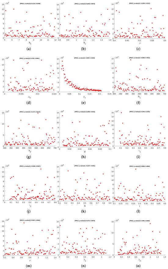
Figure A1.
PRCC plots for infected vectors.
References
- Ahmad, S.; ur Rahman, M.; Arfan, M. On the analysis of semi-analytical solutions of Hepatitis B epidemic model under the Caputo-Fabrizio operator. Chaos Solitons Fractals 2021, 146, 110892. [Google Scholar] [CrossRef]
- Colwell, R.R. Global climate and infectious disease: The cholera paradigm. Science 1996, 274, 2025–2031. [Google Scholar] [CrossRef] [PubMed]
- Keiding, J.; World Health Organization. Division of Vector Biology and Control. In The House-Fly: Biology and Control; Technical report; World Health Organization: Geneva, Switzerland, 1986. [Google Scholar]
- Graczyk, T.K.; Knight, R.; Gilman, R.H.; Cranfield, M.R. The role of non-biting flies in the epidemiology of human infectious diseases. Microbes Infect. 2001, 3, 231–235. [Google Scholar] [CrossRef]
- Greenberg, B. Flies and Disease: II. Biology and Disease Transmission; Princeton University Press: Princeton, NJ, USA, 2019. [Google Scholar] [CrossRef]
- Das, P.; Mukherjee, D.; Sarkar, A. Study of a carrier dependent infectious disease—cholera. J. Biol. Syst. 2005, 13, 233–244. [Google Scholar] [CrossRef]
- Fotedar, R. Vector potential of houseflies (Musca domestica) in the transmission of Vibrio cholerae in India. Acta Trop. 2001, 78, 31–34. [Google Scholar] [CrossRef]
- World Health Organization. Cholera vaccines: WHO position paper—August 2017. Wkly. Epidemiol. Rec. 2017, 92, 477–498. [Google Scholar]
- Losonsky, G.A.; Lim, Y.; Motamedi, P.; Comstock, L.E.; Johnson, J.A.; Morris, J.G., Jr.; Tacket, C.O.; Kaper, J.B.; Levine, M.M. Vibriocidal antibody responses in North American volunteers exposed to wild-type or vaccine Vibrio cholerae O139: Specificity and relevance to immunity. Clin. Diagn. Lab. Immunol. 1997, 4, 264–269. [Google Scholar] [CrossRef]
- Charnley, G.E.; Kelman, I.; Murray, K.A. Drought-related cholera outbreaks in Africa and the implications for climate change: A narrative review. Pathog. Glob. Health 2022, 116, 3–12. [Google Scholar] [CrossRef]
- Hailegiorgis, A.; Crooks, A.T. Agent-based modeling for humanitarian issues: Disease and refugee camps. In Proceedings of the Computational Social Science Society of America Conference, Santa Fe, NM, USA, 18–21 September 2012. [Google Scholar]
- Chowdhury, F.; Rahman, M.A.; Begum, Y.A.; Khan, A.I.; Faruque, A.S.; Saha, N.C.; Baby, N.I.; Malek, M.; Kumar, A.R.; Svennerholm, A.M.; et al. Impact of rapid urbanization on the rates of infection by Vibrio cholerae O1 and enterotoxigenic Escherichia coli in Dhaka, Bangladesh. PLoS Negl. Trop. Dis. 2011, 5, e999. [Google Scholar] [CrossRef]
- Huppert, A.; Katriel, G. Mathematical modelling and prediction in infectious disease epidemiology. Clin. Microbiol. Infect. 2013, 19, 999–1005. [Google Scholar] [CrossRef]
- Khan, M.A.; Ullah, S.; Ching, D.; Khan, I.; Ullah, S.; Islam, S.; Gul, T. A mathematical study of an epidemic disease model spread by rumors. J. Comput. Theor. Nanosci. 2016, 13, 2856–2866. [Google Scholar] [CrossRef]
- Ameen, I.; Baleanu, D.; Ali, H.M. An efficient algorithm for solving the fractional optimal control of SIRV epidemic model with a combination of vaccination and treatment. Chaos Solitons Fractals 2020, 137, 109892. [Google Scholar] [CrossRef]
- Khan, T.; Ahmad, S.; Zaman, G. Modeling and qualitative analysis of a hepatitis B epidemic model. Chaos Interdiscip. J. Nonlinear Sci. 2019, 29, 103139. [Google Scholar] [CrossRef]
- Allen, L.J.; Burgin, A.M. Comparison of deterministic and stochastic SIS and SIR models in discrete time. Math. Biosci. 2000, 163, 1–33. [Google Scholar] [CrossRef] [PubMed]
- Maliyoni, M.; Chirove, F.; Gaff, H.D.; Govinder, K.S. A stochastic tick-borne disease model: Exploring the probability of pathogen persistence. Bull. Math. Biol. 2017, 79, 1999–2021. [Google Scholar] [CrossRef]
- Maliyoni, M. Probability of disease extinction or outbreak in a stochastic epidemic model for west nile virus dynamics in birds. Acta Biotheor. 2021, 69, 91–116. [Google Scholar] [CrossRef]
- Roberts, M.; Andreasen, V.; Lloyd, A.; Pellis, L. Nine challenges for deterministic epidemic models. Epidemics 2015, 10, 49–53. [Google Scholar] [CrossRef]
- Marwa, Y.M.; Mbalawata, I.S.; Mwalili, S.; Charles, W.M. Stochastic dynamics of cholera epidemic model: Formulation, analysis and numerical simulation. J. Appl. Math. Phys. 2019, 7, 1097–1125. [Google Scholar] [CrossRef]
- Renard, P.; Alcolea, A.; Ginsbourger, D. Stochastic versus deterministic approaches. In Environmental Modelling: Finding Simplicity in Complexity; John Wiley & Sons: Hoboken, NJ, USA, 2013; pp. 133–149. [Google Scholar] [CrossRef]
- Ji, C.; Jiang, D.; Shi, N. The behavior of an SIR epidemic model with stochastic perturbation. Stoch. Anal. Appl. 2012, 30, 755–773. [Google Scholar] [CrossRef]
- Bibi Ruhomally, Y.; Zaid Dauhoo, M.; Dumas, L. Stochastic modelling of marijuana use in Washington: Pre- and post-Initiative-502 (I-502). IMA J. Appl. Math. 2022, 87, 1121–1150. [Google Scholar] [CrossRef]
- Allen, L.J. A primer on stochastic epidemic models: Formulation, numerical simulation, and analysis. Infect. Dis. Model. 2017, 2, 128–142. [Google Scholar] [CrossRef] [PubMed]
- Anteneh, L.M.; Kakaï, R.G. Mathematical modelling and analysis of cholera dynamics via vector transmission. Commun. Math. Biol. Neurosci. 2024, 2024, 74. [Google Scholar] [CrossRef]
- Akhi, A.A.; Kamrujjaman, M.; Nipa, K.F.; Khan, T. A continuous-time Markov chain and stochastic differential equations approach for modeling malaria propagation. Healthc. Anal. 2023, 4, 100239. [Google Scholar] [CrossRef]
- Allen, L.J.; Lahodny, G.E., Jr. Extinction thresholds in deterministic and stochastic epidemic models. J. Biol. Dyn. 2012, 6, 590–611. [Google Scholar] [CrossRef]
- Nipa, K.F.; Allen, L.J. The Effect of Demographic Variability and Periodic Fluctuations on Disease Outbreaks in a Vector–Host Epidemic Model. Infect. Dis. Our Planet 2021, 15–35. [Google Scholar] [CrossRef]
- Bacaër, N.; Ait Dads, E.H. On the probability of extinction in a periodic environment. J. Math. Biol. 2014, 68, 533–548. [Google Scholar] [CrossRef] [PubMed]
- Npa, K.F.; Jang, S.R.J.; Allen, L.J. The effect of demographic and environmental variability on disease outbreak for a dengue model with a seasonally varying vector population. Math. Biosci. 2021, 331, 108516. [Google Scholar] [CrossRef]
- Zevika, M.; Soewono, E. Deterministic and stochastic CTMC models from Zika disease transmission. AIP Conf. Proc. 2018, 1937, 020023. [Google Scholar] [CrossRef]
- Marwa, Y.M.; Mbalawata, I.S.; Mwalili, S. Continuous time markov chain model for cholera epidemic transmission dynamics. Int. J. Stat. Probab. 2019, 8, 1–32. [Google Scholar] [CrossRef]
- Gani, J.; Swift, R. Deterministic and stochastic models for the spread of cholera. ANZIAM J. 2009, 51, 234–240. [Google Scholar] [CrossRef]
- Azaele, S.; Maritan, A.; Bertuzzo, E.; Rodriguez-Iturbe, I.; Rinaldo, A. Stochastic dynamics of cholera epidemics. Phys. Rev. E—Stat. Nonlinear Soft Matter Phys. 2010, 81, 051901. [Google Scholar] [CrossRef]
- Witbooi, P.J.; Muller, G.E.; Ongansie, M.B.; Ahmed, I.H.; Okosun, K.O. A stochastic population model of cholera disease. Discret. Contin. Dyn. Syst.-Ser. S 2022, 15, 441–456. [Google Scholar] [CrossRef]
- Islam, M.R.; Oraby, T.; McCombs, A.; Chowdhury, M.M.; Al-Mamun, M.; Tyshenko, M.G.; Kadelka, C. Evaluation of the United States COVID-19 vaccine allocation strategy. PLoS ONE 2021, 16, e0259700. [Google Scholar] [CrossRef]
- Thul, L.; Powell, W. Stochastic optimization for vaccine and testing kit allocation for the COVID-19 pandemic. Eur. J. Oper. Res. 2023, 304, 325–338. [Google Scholar] [CrossRef]
- Cohn, J.N.; Johnson, G.; Ziesche, S.; Cobb, F.; Francis, G.; Tristani, F.; Smith, R.; Dunkman, W.B.; Loeb, H.; Wong, M.; et al. A comparison of enalapril with hydralazine–isosorbide dinitrate in the treatment of chronic congestive heart failure. N. Engl. J. Med. 1991, 325, 303–310. [Google Scholar] [CrossRef]
- Van den Driessche, P.; Watmough, J. Reproduction numbers and sub-threshold endemic equilibria for compartmental models of disease transmission. Math. Biosci. 2002, 180, 29–48. [Google Scholar] [CrossRef] [PubMed]
- Allen, L.J. An Introduction to Stochastic Processes with Applications to Biology; CRC Press: Boca Raton, FL, USA, 2010. [Google Scholar]
- Maity, S.; Mandal, P.S. A comparison of deterministic and stochastic plant-vector-virus models based on probability of disease extinction and outbreak. Bull. Math. Biol. 2022, 84, 41. [Google Scholar] [CrossRef]
- Khan, A.; Hassan, M.; Imran, M. The effects of a backward bifurcation on a continuous time Markov chain model for the transmission dynamics of single strain dengue virus. Appl. Math. 2013, 4, 663–674. [Google Scholar] [CrossRef]
- Allen, L.J.; van den Driessche, P. Relations between deterministic and stochastic thresholds for disease extinction in continuous-and discrete-time infectious disease models. Math. Biosci. 2013, 243, 99–108. [Google Scholar] [CrossRef]
- Lahodny, G.E.; Allen, L.J. Probability of a disease outbreak in stochastic multipatch epidemic models. Bull. Math. Biol. 2013, 75, 1157–1180. [Google Scholar] [CrossRef]
- Lahodny, G., Jr.; Gautam, R.; Ivanek, R. Estimating the probability of an extinction or major outbreak for an environmentally transmitted infectious disease. J. Biol. Dyn. 2015, 9, 128–155. [Google Scholar] [CrossRef]
- Kundu, S.; Jana, D.; Maitra, S. Study of a multi-delayed SEIR epidemic model with immunity period and treatment function in deterministic and stochastic environment. Differ. Equations Dyn. Syst. 2021, 32, 221–251. [Google Scholar] [CrossRef]
- Schmidt, R.; Voigt, M.; Mailach, R. Latin hypercube sampling-based Monte Carlo simulation: Extension of the sample size and correlation control. In Uncertainty Management for Robust Industrial Design in Aeronautics: Findings and Best Practice Collected During UMRIDA, a Collaborative Research Project (2013–2016) Funded by the European Union; Springer: Cham, Switzerland, 2019; pp. 279–289. [Google Scholar] [CrossRef]
- Rajabi, M.M.; Ataie-Ashtiani, B.; Janssen, H. Efficiency enhancement of optimized Latin hypercube sampling strategies: Application to Monte Carlo uncertainty analysis and meta-modeling. Adv. Water Resour. 2015, 76, 127–139. [Google Scholar] [CrossRef]
- Benedetti, L.; Claeys, F.; Nopens, I.; Vanrolleghem, P.A. Assessing the convergence of LHS Monte Carlo simulations of wastewater treatment models. Water Sci. Technol. 2011, 63, 2219–2224. [Google Scholar] [CrossRef]
- Pennington, H.M. Applications of Latin Hypercube Sampling Scheme and Partial Rank Correlation Coefficient Analysis to Mathematical Models on Wound Healing. Bachelor’s Thesis, Western Kentucky University, Bowling Green, KY, USA, 2015. [Google Scholar]
- Blower, S.M.; Hartel, D.; Dowlatabadi, H.; Anderson, R.M.; May, R.M. Drugs, sex and HIV: A mathematical model for New York City. Philos. Trans. R. Soc. Lond. Ser. B Biol. Sci. 1991, 331, 171–187. [Google Scholar] [CrossRef]
- Marino, S.; Hogue, I.B.; Ray, C.J.; Kirschner, D.E. A methodology for performing global uncertainty and sensitivity analysis in systems biology. J. Theor. Biol. 2008, 254, 178–196. [Google Scholar] [CrossRef] [PubMed]
- Helton, J.C.; Davis, F.J. Latin hypercube sampling and the propagation of uncertainty in analyses of complex systems. Reliab. Eng. Syst. Saf. 2003, 81, 23–69. [Google Scholar] [CrossRef]
- Gillespie, J.; Marshall, R.C. Proteins of the hard keratins of echidna, hedgehog, rabbit, ox and man. Aust. J. Biol. Sci. 1977, 30, 401–410. [Google Scholar] [CrossRef]
- Kadaleka, S. Assessing the Effects of Nutrition and Treatment in Cholera Dynamics: The Case of Malawi. Master’s Dissertation, University of Der es Salaam, Dar es Salaam, Tanzania, 2011. [Google Scholar]
- Onuorah, M.O.; Atiku, F.; Juuko, H. Mathematical model for prevention and control of cholera transmission in a variable population. Res. Math. 2022, 9, 2018779. [Google Scholar] [CrossRef]
- ELmojtaba, I.M.; Biswas, S.; Chattopadhyay, J. Global dynamics and sensitivity analysis of a vector-host-reservoir model. Sultan Qaboos Univ. J. Sci. [SQUJS] 2016, 21, 120–138. [Google Scholar] [CrossRef]
- Hartley, D.M.; Morris, J.G., Jr.; Smith, D.L. Hyperinfectivity: A critical element in the ability of V. cholerae to cause epidemics? PLoS Med. 2006, 3, e7. [Google Scholar] [CrossRef]
- Modnak, C. A model of cholera transmission with hyperinfectivity and its optimal vaccination control. Int. J. Biomath. 2017, 10, 1750084. [Google Scholar] [CrossRef]
- Al-Shanfari, S.; ELmojtaba, I.M.; Alsalti, N. The role of houseflies in cholera transmission. Commun. Math. Biol. Neurosci. 2019, 2019, 31. [Google Scholar] [CrossRef]
- Akman, O.; Corby, M.R.; Schaefer, E. Examination of models for cholera: Insights into model comparison methods. Lett. Biomath. 2016, 3, 93–118. [Google Scholar] [CrossRef]
- Marwa, Y.M.; Mwalili, S.; Mbalawata, I.S. Markov chain Monte Carlo analysis of cholera epidemic. J. Math. Comput. Sci. 2018, 8, 584–610. [Google Scholar] [CrossRef]
- Isere, A.; Osemwenkhae, J.; Okuonghae, D. Optimal control model for the outbreak of cholera in Nigeria. Afr. J. Math. Comput. Sci. Res. 2014, 7, 24–30. [Google Scholar] [CrossRef]
- Allen, L.J. An introduction to stochastic epidemic models. In Mathematical Epidemiology; Springer: Berlin/Heidelberg, Germany, 2008; pp. 81–130. [Google Scholar] [CrossRef]
Disclaimer/Publisher’s Note: The statements, opinions and data contained in all publications are solely those of the individual author(s) and contributor(s) and not of MDPI and/or the editor(s). MDPI and/or the editor(s) disclaim responsibility for any injury to people or property resulting from any ideas, methods, instructions or products referred to in the content. |
© 2025 by the authors. Licensee MDPI, Basel, Switzerland. This article is an open access article distributed under the terms and conditions of the Creative Commons Attribution (CC BY) license (https://creativecommons.org/licenses/by/4.0/).