Pricing and Return Strategies in Omni-Channel Apparel Retail Considering the Impact of Fashion Level

Abstract

In the context of new retail, the development of omni-channels is flourishing. The entry threshold for the clothing industry is low, and the popularity of online shopping has, to some extent, reduced consumers’ perception of the authenticity of clothing. As a result, returns are a serious issue in the clothing industry. This article focuses on a clothing retailer while addressing retail and return issues in the clothing industry. It develops and analyzes models for an online single-channel strategy and two omni-channel showroom strategies: “Experience in Store and Buy Online (ESBO)” with an experience store and “Buy Online and Return in Store (BORS)” with a physical store. These models are used to examine the pricing and return decisions of the retailer in the three strategic scenarios. Additionally, this study considers the impact of fashion trends on demand. It explores pricing and return strategies in two showroom models under the influence of the fashion trend decay factor. Moreover, sensitivity analyses and numerical analyses of the important parameters are performed. This research demonstrates the following: (1) In the case of high return transportation costs and online return hassle costs, clothing retailers can attract consumers to increase profits through establishing offline channels; (2) extending the sales time of fashionable clothing has a positive effect on profits, but blindly prolonging the continuation of the sales time will lead to a decrease in profits; (3) the larger the initial fashion level or the smaller the fashion level decay factor, the greater the optimal retailer profits. The impacts of the initial fashion level and fashion level decay factor on profits are more significant in omni-channel operations. This article aims to identify optimal strategies for retailers utilizing omni-channel operations and offer managerial insights for the sale of fashionable apparel.

1. Introduction

The development of the contemporary retail industry faces many challenges. Both traditional offline retail stores and emerging online retail stores have exposed different issues relating to terminal sales. For example, problems with offline retailing include a decline in customer traffic due to increased online shopping, as well as time and geographical constraints; meanwhile, problems with online retailing include the low credibility of product information and high return rate. As the closest link to consumers, retailing is in urgent need of omni-channel transformation due to the changing needs of consumers and the needs of the enterprises’ own development in order to enhance consumers’ shopping experiences, thereby increasing their market share and retailers’ profits. Retailers adopting multi- or omni-channel strategies will be able to offer customers seamless shopping experiences. For example, customers may browse a store’s website, select the products of their choice, and then go to an offline store to make a purchase. Sometimes, they are looking for a quick purchase and shop directly through a mobile app, while, at other times, they want a more immersive shopping experience and choose to shop in a physical store. As a result, such retailers will be better able to meet customers’ constantly changing needs and preferences through digital (or phygital) channels [1]. However, after more than a decade of theoretical research and practical application, it is still difficult to form a system for omni-channel research. The key attributes that affect the seamless consumer experience (e.g., price and returns) will vary depending on the type of retailer and the channels being integrated, and this type of research is currently underdeveloped [2]. This poses challenges to researchers and market participants promoting research and practice in this field. The retail industry involves a wide range of commodity categories, and different commodities have different characteristics. Combining commodity characteristics to innovate retail models is becoming a development trend.

With the vigorous development of e-commerce in China in the past 10 years, online sales in the clothing industry have grown from scratch, and online channels have been an important force driving the growth of the clothing industry (data source: Prospective Industry Research Institute). China’s online retail apparel sales increased by 94.92% over the six-year period from 2018 to 2023, from 1440 billion yuan to 2300 billion yuan. However, as the traffic dividend of e-commerce platforms gradually fades, the annual year-on-year growth rate of online retail sales of apparel has slowed down, dropping from a high growth rate of 22.03% in 2018 to a medium growth rate of 11.11% in 2023 (data source: China National Textile and Apparel Council). The popularity of online shopping has had a huge impact on traditional offline apparel stores, with many clothing retailers switching to online stores. However, the increase in the number of online stores has led to fierce competition, making it difficult to increase one’s market share.

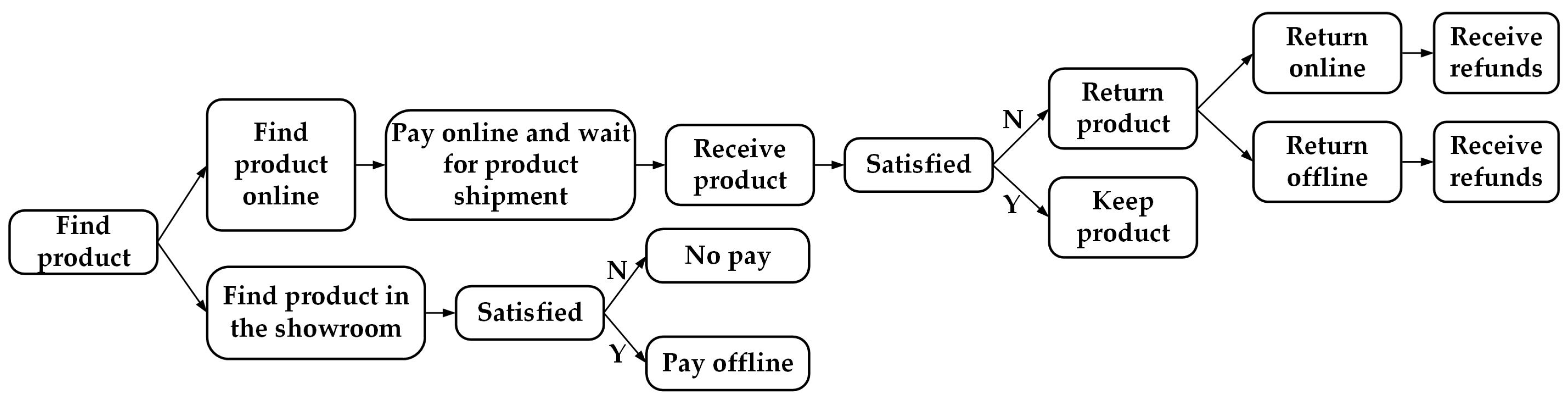
Faced with the above problems, many large apparel retailers have begun to explore new retail innovation. For example, in 2015, INMAN women’s clothing enterprises applied a “Showrooms” mode to provide offline experience stores for online stores, exploring a path for online and offline retailing in a holistic manner. By the beginning of 2021, INMAN had opened more than 600 offline experience stores in 179 cities across China, and the proportion of offline sales leveled with the proportion of online sales (data source: China Development and Reform News Agency). It can be seen that the implementation of omni-channel strategies by online retailers has significant advantages and important significance. This provides new ideas and models for the development of the retail industry and deserves to be further studied. In our study, we examine two omni-channel strategies. With the “Experience in Store and Buy Online (ESBO)” strategy, retailers open offline experience stores. Customers can visit these stores to try products and gather sufficient information about them. After that, they decide whether to purchase the products online. Returns are not accepted at the experience stores. Some retailers, such as Zara and Ikea, have opened offline experience stores to offer products for sales and display [3]. The other omni-channel strategy is the “Buy Online and Return in Store (BORS)” strategy. Retailers open physical stores offline, and allow consumers who have purchased products online to return unsatisfactory products to the physical stores. Some retailers, such as Kohl’s and Walmart, have already offered BORS services to consumers [4]. Retailers can improve their operational efficiency through implementing omni-channel operations, but this also presents a price dilemma. Retailers used to charge different prices for goods in different channels. As consumers’ omni-channel awareness grows, more and more consumers will compare prices across channels. Price-sensitive customers will prefer low-priced channels to make purchases. This presents a challenge for the progress of retailers’ omni-channel operations. Therefore, it is especially crucial to research retailers’ pricing strategies in omni-channel operations.

At the same time, consumer returns in the apparel industry are widespread and have brought many problems. People between the ages of 25 and 34 are more likely to return items that they purchase online, according to a 2023 Parcel Labs survey. Customers return all kinds of goods, including clothing, fashion products, and electronics. One of the economies that is growing the fastest is that of India. In 2022, the total return order volume in India accounted for 14.86%, where fashion and clothing items were the most often returned goods, followed by electronics [5]. A survey by SaleCycle showed that, for some consumers, returning products is only a part of the shopping experience. Customers choose to buy different variations of clothing items (e.g., sizes, colors) to try on at home as they cannot determine with certainty whether they fit before buying them online. Therefore, in order to pursue the provision of better service to consumers, many clothing retailers have implemented relatively loose return policies. This implementation has resulted in high return rates and increasing return costs for retailers. Returns, as an important part of the clothing supply chain, have gradually become a key link for retailers to improve their service levels. Many retailers no longer regard returns as a phenomenon of evasion but, instead, as one that plays a positive role in retailing by formulating innovative return strategies.

Fashion products fit current trends, bringing topics and sociality. Fashion products generate consumer attention, reviews, and discussion on social media [6], such that people show a greater preference for fashionable clothing in clothing consumption. The fashion level of apparel deteriorates with time due to seasonal and quickly changing fashion trends, and slow-selling or out-of-season items are likely to lose their value. Therefore, retailers must update entire categories every three to four months due to consumer demand and competition. Fashion has an important impact on the demand for fashionable clothing during its lifecycle. The way of choosing the right pricing strategy according to the changing fashion level of clothing is an important issue for apparel retailers. The domestic apparel brand Urban Revivo first became the sales champion for women’s clothing in China, according to a 618 list published by Tmall in 2022. The reason for the sharp rise in Urban Revivo’s sales is that they accomplish a greater level of quality than fashion at a lower price than that of luxury goods in order to guarantee high-cost performance [7]. Furthermore, developing differentiated return policies in different sales periods can provide effective strategies for retailers to solve the return problem of fashion clothing.

No previous research has examined the integrated pricing and return strategies of fashionable apparel retailers with different omni-channel models, according to a review of the literature. This study takes the impacts of different omni-channel retailing models into account. This feature sets it apart from other studies on fashionable clothing retail (e.g., Shi and You [7]) that have only concentrated on the retailer’s optimal operational strategy. This work also differs from the study by Guo et al. [8], in that it focuses on the impact of the fashion level decay on the retailer’s optimal strategies and profits. Furthermore, this study is different from earlier research on the topic of opening an offline showroom (e.g., Zhang et al. [9]), choosing an omni-channel retail mode (e.g., Mandal et al. [10]), and the optimal strategy for omni-channel retailing (e.g., Ma et al. [11]), as this study focuses on a specific apparel industry. Moreover, it takes a single apparel retailer as the subject and examines the impact of fashionable apparel products eventually becoming outdated. Therefore, in this study, we aim to explore the optimal pricing and return strategies of an apparel retailer with two different omni-channel retailing models in order to provide reference points for enterprises. In addition, considering the importance of the fashion decay factor in omni-channel apparel retailing and a small number of related literature, this study focuses on the specific aspect. It thoroughly examines the impact of changes in the fashion level of fashionable apparel and changes in demand brought about by fashion decay in the apparel retailing industry.

This work mainly focuses on the following issues.

(1) Under what conditions is it profitable for an online retailer to introduce a showroom?

(2) Under different conditions, which omni-channel retail model would be more beneficial for an apparel retailer to choose?

(3) How does the fashion level decay of fashion appeal affect the strategic decisions of the clothing retailer?

To examine these issues, this work is based on an online apparel retailer. We develop models for an online single-channel strategy and two omni-channel showroom strategies, taking returns into account: an ESBO model with an experience store and a BORS model with a physical store. We compare and analyze the pricing and return strategies before and after opening the experience store and the physical store. Additionally, we introduce the effect of the fashion level into the model to examine the pricing and return strategies of the fashionable apparel retailer while taking the influence of the fashion decay factor on the strategies of the fashionable clothing retailer into account. After constructing the demand function, we introduce the change in demand into the retailer’s profit function for a comprehensive analysis, complementing the few studies that have considered the fashion level of apparel.

The innovative points of this work are as follows. Firstly, few studies have comparatively analyzed a retailer’s pricing and return strategies with the new emerging showroom models of ESBO and BORS in omni-channel retailing. Such studies are in the initial stage of exploration, and this article enriches the relevant literature. This work analyzes the retailer’s optimal strategies before and after opening an experience store and a physical store. It compares and analyzes the two omni-channel models to provide retailers with realistic guidance on optimal pricing and return strategies. It also provides significant and realistic guidance on the omni-channel transformation for single- and dual-channel retailers. Secondly, this work aims at the phenomenon of high return rates in the apparel industry. It considers the impact of fashion level decay on the optimal strategies and profits of an apparel retailer with omni-channel retailing for the first time. We study the development of pricing and return policies over the course of the sales cycle and set differentiated return strategies to maximize the retailer’s profits. This work analyzes the impact of parameters affecting the fashion level on the retailer’s profits and the differences between the two different omni-channel showroom models. It provides omni-channel retailers with more significant managerial insights.

We make the following contributions through examining the impact of fashion level decay on the pricing and return strategies of the fashionable apparel retailer under two omni-channel retailing models. First, this article studies in depth how an apparel retailer facing the problem of high return rates can develop effective strategies with two omni-channel operation models: the experience store model and the physical store model. It comparatively analyzes the optimal strategies and retailer profits under different showroom models. Second, this study introduces the influential factor of the fashion level. It conducts further research on the omni-channel pricing and return strategies of the fashionable apparel retailer with the omni-channel models. This research fills the gap in the existing literature regarding the impact of the changing fashion level on the integrated pricing and return strategies of the omni-channel apparel retailer. This article also complements the research on the impact of fashion level decay on retailers. In addition, this article provides new analytical perspectives for solving the problem of high return rates and practical management suggestions for the return link in the apparel industry. It also provides optimal strategic choices for retailers running omni-channel operations and management insights for fashionable apparel sales. Therefore, the novelty and substantial insights of this study are not only theoretically proven but can also provide valuable reference suggestions for actual enterprises.

The findings of this study are novel and interesting. Firstly, consistent with the previous literature, retailers only choose to sell products through the online channel when return transportation costs are low [10]. For fashion retailers, their optimal profits gradually increase as the initial fashion level increases and decrease as the fashion level decay factor increases [12]. Secondly, differing from the results of previous studies, it is found that when the return transportation costs or the online return hassle costs are high, retailers can attract consumers by opening offline experience stores and physical stores. The ideal option is to open physical stores. With the optimal retail price, the positive effect on profit diminishes when the fashion level’s existence time increases to a certain value. Surprisingly, as the retail price gradually increases, retailers’ profits do not keep increasing as the continuing sales time increases. To the contrary, under certain conditions, it negatively affects retailers’ profits. In addition, while there is some literature focusing on the impact of fashion level decay on retailers’ decision making [7,12,13,14], only a very small number of studies have combined multiple omni-channel strategies. It is interesting to find that changes in fashion level have a more pronounced impact on retailers’ profits under the ESBO and the BORS strategies. Therefore, retailers who open offline experience stores and physical stores have to focus more on maintaining the fashion level. Our study effectively compares retailers’ decisions with three different retail strategies and provides meaningful references for fashionable apparel retailers’ operations.

This work includes the following sections. Section 2 provides a detailed literature review in the relevant field. The problem description, notation, and assumptions are presented in Section 3. Section 4 presents the model formulations and analyses. Section 5 presents sensitivity analyses and numerical analyses of the important parameters. Section 6 summarizes the main conclusions of the study and discusses future considerations. Furthermore, the proofs are presented in Appendix A.

2. Literature Review

In this section, we review the streams of the literature related to the research content, which are divided into the following three directions: omni-channel strategies, clothing pricing strategies, and clothing return strategies.

2.1. Omni-Channel Strategies

The term “omni-channel” refers to breaking down barriers and providing consistent service across online and offline channels. Iglesias-Pradas and Acquila-Natale [1] systematically examined different areas of multi-channel and omni-channel retailing. In research on omni-channel retailing, “Showrooms” are a hot topic. In the existing literature, some studies have focused on one retailer to illustrate the advantages of opening a showroom. Bell et al. [15] empirically demonstrated that introducing showrooms can not only reduce customer returns but also increase online and offline sales. Kumar et al. [16] explored how establishing a new physical store can affect the demand for the existing online channel and the revenue of retailers. Through analyzing customer-level data from a clothing retailer, they found that such a strategy does indeed increase online sales and the retailer’s revenue. Mahar et al. [17] developed a mathematical model that examined the value of the costs of providing pickup in store and return services, and they indicated that not all retail stores should provide pickup in store and/or return services. Some scholars have studied two retailers to illustrate the advantages of the Showrooms model. For example, Basak et al. [18] analyzed multi-channel retail operations in the context of Showrooms, determined pricing strategies for traditional retailers and online retailers, and proposed the view that showrooms are beneficial to online retailers and unfavorable to traditional retailers. Fan et al. [19] divided showrooms into those for display and sales based on their different functions, and they analyzed the issue of whether showrooms should be used for display or sales through game research between two competing retailers. Furthermore, some scholars have included manufacturers among their research subjects. Li et al. [20] analyzed the service effort strategies of physical showroom retailers in a dual-channel supply chain in response to the conflict between manufacturers’ online channels and retailers’ offline channels, and they studied the pricing strategies for each strategy and their impacts on the entire supply chain.

With the further development of practice and theoretical research, many types of showrooms have emerged. Many studies have focused on different types of showrooms. Li et al. [21] studied the impacts of different physical showroom deployment strategies on the information service provision, pricing, and profitability of an omni-channel retailer. There were no showrooms, partially classified showrooms, and fully classified showrooms. This work focuses on the model of showrooms with experience, which means that there is no inventory in the showroom. This type of showroom is increasingly favored in the development of omni-channel retailing. Gao and Su [22] studied three different information-sharing methods; namely, physical showrooms, virtual showrooms, and availability information disclosure. One of the research conclusions is that physical showrooms may encourage retailers to reduce their store inventory. Bell et al. [23] studied zero-inventory showrooms (ZIS) and found that after experiencing ZISs, customers spent more, shopped faster, and had a lower likelihood of returns. The positive impact on returns is doubly virtuous, as it is more pronounced for products that are more tactile and higher-priced, thereby mitigating a key pain point in online retail.

In addition, some of the previous literature has examined the ESBO and BORS omni-channel models separately. In terms of ESBO strategies, Cao et al. [3] used a parsimonious model to analyze the impact of inspection provision on the interactions between a retailer and strategic consumers; that is, the impact of the ESBO strategy on store operations. Gong et al. [24] constructed profit maximization models for online retailers implementing a single online strategy and online and ESBO strategies, and then they introduced live streaming into the models to comparatively analyze the impact of live streaming on demand and profit. In terms of BORS strategies, considering two supply chains selling the same products in the same market, Huang and Jin [25] explored the BORS strategy’s impact from a competitive perspective. They found that a competitive environment would make retailers prefer to offer BORS under almost all conditions. Yan et al. [26] considered two competing dual-channel retailers and examined the optimal conditions for one or both of them to offer a BORS strategy in order to test whether it is beneficial to introduce a BORS strategy in a competitive market. Yang et al. [27] considered retailers who sell products through online and in-store channels to customers who are unsure of the products’ suitability. They examined the impact of BORS on retailers’ operations in terms of the customer base, inventory decisions, and expected profits. However, studies that have examined and comparatively analyzed both ESBO and BORS strategies are less common. Mandal et al. [10] studied both ESBO and BORS omni-channel configuration methods, starting with omni-channel configuration strategies, to provide the best solution for online retailers selling different types of products.

The apparel industry is an industry with obvious characteristics of the new retail transformation. In recent years, many literature reviews have begun to focus on retail in the fashion industry. Wen et al. [28] recognized the importance of fashion retail supply chain management (FRSCM) and reviewed the relevant literature on channel selection for fashion retailers, emphasizing that channel selection is one of the important research directions in fashion retail. Some scholars have conducted empirical studies on omni-channel retailing in the apparel industry. Kanat and Atilgan [29] studied consumer-preferred omni-channel implementations in the clothing sector and used statistical methods, such as exploratory factor analysis, t-tests, and analyses of variance, to examine the relationships between omni-channel implementations. Liu and Liu [30] aimed to clarify the effect of cross-channel consistency on brand loyalty and trust. They gathered information from customers of multi-channel apparel brands, and the findings showed that product and service consistency positively influenced brand loyalty via brand trust, whereas price and promotion consistency did not. It can be seen that there is currently a limited number of studies in the research literature focusing on omni-channel models in the fashionable clothing industry. Most of the existing literature on omni-channel apparel retailing are empirical, while there are fewer studies on related theoretical strategies. In addition, some studies do not fully reflect the characteristics of the clothing industry. Therefore, research in this field still needs to be continuously deepened.

Combing the literature on omni-channel strategies, we find that research on omni-channel showrooms is currently a popular direction. However, the majority of studies are aimed at different showroom models. Most studies on showrooms involve a retailer and a manufacturer, while few studies in the literature are only aimed at the retail segment. In addition, a small number of studies carried out in-depth analyses of different showroom modes. There is no unified standard for the classification of several showroom models, and there is a lack of studies on the differences among different types of showrooms. There is some literature that examines the ESBO and BORS strategies separately, but less of the literature examines both of the two strategies simultaneously. Moreover, there are only a few studies on omni-channel retail exploring the apparel industry, and most of the existing related literature focuses on empirical research rather than theoretical studies. In order to address this issue, this study takes a clothing retailer as the research object, dividing offline-channel showrooms into experience stores and physical stores. It systematically models and analyzes the two types of showroom modes to explore the retailer’s optimal strategies and profits with different omni-channel modes.

2.2. Clothing Pricing Strategies

The pricing of clothing is a crucial component in the operation of apparel products; thus, numerous scholars have studied pricing issues in the apparel industry. Some scholars have discussed optimal pricing strategies for apparel supply chains in depth from different perspectives. Wang et al. [31] concentrated on how information sharing and the showroom phenomenon affected the prices and services in a multi-channel apparel supply chain. Ma and Wang [32] constructed static and dynamic game models based on the centralized and decentralized decision-making modes, in order to explore the optimal pricing strategies for an apparel supply chain from the viewpoints of low-carbon investment and consumers’ low-carbon preferences. Cao and Ji [33] concentrated on an apparel brand’s recycling pricing strategy, believing that it influences both the reverse channel in a closed-loop supply chain and the consumer demand in the forward channel. Some studies have focused on price reduction strategies for apparel products. Namin et al. [34] developed a model for pricing seasonal commodities to help retailers better cope with demand uncertainty. They estimated this using a finite mixture model with data from a leading specialty apparel company and found that the retailer should implement middle-of-the-season price markdowns for products that have high initial prices, are introduced in the summer/fall, or have darker colors. Cosgun et al. [35] constructed a markdown optimization model that takes the cross-price effects in a random demand setting for multi-product groups into account while addressing the simultaneous determination of markdown prices and optimal initial inventory levels for an apparel retailer in Turkey.

It is worth noting that many studies on pricing strategies for apparel have ignored that fashionable apparel will become less fashionable over time. In the last few years, some scholars have begun to pay attention to the issue of fashion level decay, further supplementing the research on pricing strategies, inventory strategies, and other issues in the clothing industry. The concept of fashion level decay originates from deterioration. The life cycle of fashionable clothing is very short, and the change in the market value of the fashionable clothing is similar to that of deteriorated products. Similarly to perishable products, the freshness of fresh products decreases over time [36,37,38], which is an important factor affecting consumer purchasing decisions. Tsiros and Heilman [39] studied how consumers’ purchase intentions are affected by the product expiration date, and they reported that their purchase intentions decrease throughout products’ lifetimes. Undoubtedly, a higher freshness or fashion level helps to improve the demand for perishable products. Then, Herbon [40] proposed an inventory model with regular replenishment, where consumers have different sensitivities to product freshness. The demand function includes factors such as price impact, freshness, and consumer combination. Subsequently, Herbon [41] discussed the optimal piecewise constant price with heterogeneous sensitivity to product freshness. Shi and You [7] introduced a reference value to represent consumers’ requirements for the fashion level, and discussed a dynamic pricing and investment strategy for fashion products that decay in value, such as fashion clothing.

The previous literature related to fashionable apparel pricing discusses different fashion level decay models. Chen and Xu [13] considered a dynamic two-level fashionable apparel supply chain. In their study, differential equations were used to characterize the dynamics of fashion level and goodwill, and the design innovation investment was introduced into the fashion level change equation. Exponential decay models for the fashion level are the most common. Lu and Yan [14] considered the impacts of dynamic fashion trends and stochastic factors on inventory. They proposed that the fashion level function takes a monotonically decreasing exponential form, and they used Brownian motion to model the fashion level function as a stochastic process. Their study examined the managerial characteristics associated with fashion products when the fashion level is disturbed by simple random factors. Shi et al. [12] introduced the concept of the fashion level in the pricing and production strategies of fashion brands considering pre-sale and regular sales stages. They use an exponential decay model to describe changes in clothing’s fashion level over time, reflecting the popularity of clothing in the market.

Most previous studies on pricing strategies for apparel products focus on the apparel supply chain. However, the number of studies focusing on apparel retailers is relatively small, and some do not adequately reflect the characteristics of the apparel industry. Furthermore, clothing can be divided into evergreen and fashion categories. Fashionable clothing has its own fashion characteristics, making research on it more complex. The way of choosing appropriate pricing strategies based on changes in fashion level is an important issue faced by clothing retailers. In existing studies on fashionable apparel, the fashion level has been proposed and has become a hot topic for research in recent years. However, the current related studies are relatively simple, and their number is small. Moreover, among the fashion level decay models, the exponential decay model is the most classical and common. This study introduces the fashion level into the examination of pricing and return strategies for fashionable apparel. It innovatively analyzes the impact of parameters affecting the fashion level on the comprehensive strategies of the fashionable apparel retailer, enriching the management insights based on the existing literature.

2.3. Clothing Return Strategies

As an important part of a reverse logistics system, customer return is a very important issue for retailers. Some scholars focused on researching return strategies. Martinez-Lopez et al. [42] investigated the strategies of using return credits (a maximum free return amount) to reduce returns and the negative effects of doing so, in order to help online retailers decide whether or not to introduce return credits to manage returns and help them design the return credits. Additionally, some scholars concentrated on the niche research field of omni-channel return strategies. Nageswaran et al. [43] examined the return policy decisions of an omni-channel retailer. They found that omni-channel firms with good online return recovery partners and firms with more brick-and-mortar customers should offer full refunds, while firms with a significant store network and better in-store recycling opportunities may be better off charging for online returns. Some scholars have discussed the impacts of consumer behaviors on return policies. For example, Lin et al. [44] developed an analytical model based on consumer utility theory to study retailers’ optimal return–freight insurance policies. Liu et al. [45] considered that consumers engage in social learning by referring to other people’s reviews. The study concluded that partial-refund policies tend to be more favorable to sellers than full-refund and no-refund policies in the context of social learning. Some scholars paid more attention to consumers’ perceived risk in returns. Shao et al. [46] developed a theoretical model of the impact of return policy leniency on consumers’ purchase intentions in the context of cross-border e-commerce, and the results showed that the mediating role of consumers’ perceived quality and perceived risk is significant. Rokonuzzaman et al. [47] explored the important role of retailers’ return policies on consumers’ decision making. They found that liberal return policies reduce consumers’ perceived purchase risk and make them increase their willingness to patronize stores.

Some scholars studied the impact of returns on pricing or ordering strategies. Goedhart et al. [48] modeled and analyzed an omni-channel retailer’s rationing and ordering decisions by integrating them into a Markov decision process (MDP) that maximizes the retailer’s profit while taking the uncertainty of product returns into account. They discovered that the offline channel’s profit and service quality are negatively impacted by an increase in online returns. Guo et al. [49] proposed flexible return strategies considering demand uncertainty to coordinate the supply chain risk caused by demand uncertainty. On the basis of this, they explored the optimal pricing and ordering strategies for supply chain participants. The joint study of pricing strategies and return strategies can comprehensively provide guidance and suggestions for retailers to develop retail strategies. For example, Ma et al. [11] examined the relationship between return losses and customer perceptions of online products and analyzed how these factors affect the optimal return strategy and channel pricing for profit-maximizing omni-channel retailers. Their analysis identified situations where a specific return strategy either increased or decreased retailer profit, thereby facilitating optimal channel pricing decisions.

As returns are very frequent in the apparel industry, many scholars have conducted empirical studies on the subject. Using a literature study and a case study, Leeuw et al. [50] investigated how online apparel retailers make trade-offs in the efficiency of processing consumer returns to lower the quantity of returns and boost sales through return management. Kalpoe [51] predicts consumers’ acceptance of several technological alternatives based on the context of garment e-commerce that are designed to boost online purchase successes and decrease unnecessary apparel returns. Kaushik et al. [52] used the best–worst method to prioritize and rank 34 factors of online returns more effectively based on the high rates of online clothing returns. The study showed that the important factors for online clothing returns included size variation, defects, superior products, incorrect product delivery, and lenient return policies. A few scholars studied the impact of returns on the optimal strategies of apparel companies. In order to examine how retail competition and customer returns impact the development of green fashionable apparel products, Guo et al. [8] established a fashion supply chain with a manufacturer and two competing retailers. They discovered that an increase in the consumer return rate significantly lowered the optimal product greenness level. Xu et al. [53] observed consumers’ bracketing purchase behavior for clothing products, but the phenomena of returns triggered by the behavior posed a significant challenge for online retailers. They created models that maximized retailers’ profits to explore the optimal retailing and ordering strategies. According to this study, retailers should order more products to meet consumer demand when profits are negatively impacted by a high volume of returned goods.

In conclusion, the majority of the previous literature on returns has focused on three aspects. One is research on return strategies, and another is the effect of returns on pricing and ordering strategies. The third is the optimal integrated decisions for retailers combining price and return strategies. At present, research on integrated strategies is a relatively new area of study that takes more complicated and practical difficulties into account. It is worth noting that there are fewer relevant theoretical studies in the majority of the literature on returns for clothing retailers, which focuses on empirical research. Furthermore, in theoretical research on optimal operational strategies in the clothing industry, more scholars have examined how return circumstances affect the optimal manufacturing or ordering strategies of clothing companies. However, only a small number of studies have focused on optimal return policies for clothing retailers. Therefore, this work organically combines the theory and practice of the return link to compensate for the shortcomings of the relevant literature. With omni-channel retailing strategies, we examine an apparel retailer’s options for integrated pricing and return strategies when opening a showroom.

2.4. Summary of the Related Research

Overall, research on omni-channel strategies—particularly showrooms—is a crucial area of study in the retail sector according to our comprehensive review and analysis of the relevant literature. Relevant studies have examined valuable issues, such as the benefits of opening a showroom and the different types of showrooms. However, only a small number of studies have examined omni-channel operations in the retail sector, and even fewer have compared and analyzed different showroom models. Within the scope of the apparel industry, only a few scholars have examined the omni-channel retailing of clothing. The majority of existing relevant studies are reviews and empirical research and, so, there is still much space for theoretical research to work as a supplement. Given the research gaps and shortcomings in the previous literature, this study analyzes the fashion industry. This study makes contributions to the literature on omni-channel apparel retailing. It focuses on comparing and analyzing the optimal strategies of clothing retailers with two models—the ESBO strategy and the BORS strategy—that are popular among multiple omni-channel strategies and are widely used in practice. Furthermore, pricing and returns are significant issues for clothing retailers and are essential to their operational efficiency. The majority of studies on clothing pricing ignore how retailers’ pricing strategies are affected by the fact that clothing products’ fashion level deteriorates over time. The majority of earlier research on clothing returns has been empirical, with few theoretical studies. The majority of authors of related theoretical studies concentrate on how return situations affect the optimal operational strategies of clothing retailers, while the optimal return strategies of retailers have received little attention. Therefore, this study combines the research foundation of the previous literature and introduces the fashion degree into the models for further research. It thoroughly examines the retailer’s optimal pricing and return strategies and focuses on how the attenuation of the fashion degree impacts the apparel retailer’s best strategies. Research on returns has different perspectives. This study is concerned with the positive aspects of returns. It aims to provide retailers with solutions to deal with the problem of high return rates through innovative return strategies to improve their profits.

The differences between our work and previous studies are presented in

Table 1. Key related studies in the literature.

Key Related Literature	Apparel	Pricing	Markdown	Return	Fashion Level	Omni-Channel	Showrooms
Shi, You [7]	✓	✓			✓
Guo et al. [8]	✓	✓		✓
Mandal et al. [10]		✓		✓		✓	✓
Ma et al. [11]		✓		✓		✓	✓
Shi et al. [12]	✓	✓			✓
Basak et al. [18]		✓					✓
Li et al. [20]		✓					✓
Li et al. [21]		✓				✓	✓
Namin et al. [34]	✓	✓	✓
Cosgun et al. [35]	✓	✓	✓
Lu, Yan [14]	✓	✓			✓
This study	✓	✓		✓	✓	✓	✓

.

3. Problem Description and Assumptions

In this article, we examine the “Buy Online and Return Online (BORO)” single-channel strategy and two omni-channel strategies that reduce the risk of consumers buying online. One omni-channel strategy is the “Experience in Store and Buy Online (ESBO)” strategy. In addition to digital channels, retailers can open “showrooms” where customers can gather the product information that they need to buy online. Therefore, this strategy can significantly reduce the return rate of products. The other increasingly popular omni-channel strategy is the “Buy Online and Return in Store (BORS)” strategy, which allows consumers to return products to the offline stores. Therefore, the presence of physical stores will significantly reduce the retailers’ return processing costs. Both of these omni-channel strategies can offset the negative impact of product returns and increase overall sales for retailers.

In the context, this study takes an apparel retailer as the research object and establishes an online single-channel retailing (BORO) model, an ESBO omni-channel model, and a BORS omni-channel model. Given that different retail models can affect the retailer’s optimal strategic choices, this study examines the retailer’s pricing strategies, return strategies, and profitability with these three retail models. Then, considering the fashion level decay of apparel products, we introduce the fashion level into the models to explore how it affects the retailer’s optimal strategies and profits. The purpose of this study is to help fashionable apparel retailers make their omni-channel model choices and the optimal strategies in order to maximize their profits in different situations.

3.1. Problem Description

As a benchmark, we first analyze the situation in which the retailer operates online channels only. We call this strategy BORO. With this model, if consumers buy products from online channels, they cannot evaluate certain features of the products. Consumers can collect product information through online comments and other ways. However, once they receive the product, they will decide whether to return it based on whether the product conforms to and fits their requirements. With probability $\theta$, the consumer likes the product and keeps it. With probability $1-\theta$, they are dissatisfied with the product and return it. For each return unit, retailers will charge a certain return penalty f in different ways. Retailers usually charge such a penalty to reduce consumers’ returns [54,55,56]. For example, H&M charges $5.99 as a restocking fee. At the same time, some retailers do not charge explicit penalties but charge implicit return penalties by raising the retail price, providing non-full refunds, etc.

In the ESBO omni-channel model, consumers can make purchases online after experiencing products in an offline experience store. Some online retailers have established physical showrooms or experience stores. They display some sample items to help consumers reduce the uncertainty of mismatches and returns in retail. Figure 1 shows consumers’ purchasing process with the ESBO omni-channel strategy. Retailers provide a special type of offline service in the experience store, where customers can physically examine and test products [15,21]. However, consumers cannot purchase these products from the experience store. If consumers like a product after evaluating it in the experience store, they can purchase products through the online channel, and no return will be made after purchasing in this way. Compared with a conventional physical store, consumers visit the experience store only for experience and trials with products, so it requires less floor space and, therefore, lower infrastructure costs. The unit fixed facility cost of setting up an experience store is given by $F_1$.

In the BORS omni-channel model, consumers can purchase products directly in-store, and they are allowed to return products that they have bought online to offline stores. Figure 2 shows consumers’ purchasing process with the BORS omni-channel strategy. With this strategy, consumers can purchase products from both online and offline channels, and there is no return issue for products purchased offline. Customers who buy products online have the option to return them either online or in-store.

3.2. Notation and Assumptions

The customer incurs a hassle cost $h_o\ge 0$ from buying a product online, such as the cost of online browsing inconvenience, waiting time, and concerns about delivery [57]. The customer incurs a hassle cost $h_{ro}\ge 0$ while returning the product [43,58,59]. The online return penalty f can be the return transportation costs that consumers have to bear or the loss of a non-full refund. Only $0\le f\le p$ consumers have the motivation to return [10,27]. The probability that the product matches a customer’s preference is $\theta$ (0 < $\theta$ < 1); then, $1-\theta$ is the probability that the product does not match, i.e., the return rate of the product [10,24]. All model parameters are listed in

Table 2. Notations for parameters and variables.

Symbol	Description
Parameters
c	Unit production cost to a retailer
$\theta$	Probability with which the product conforms to a customer’s preference
v	Valuation of the product when it matches a customer’s preference
r	Unit return transportation cost to a retailer
$u_o^i$	Customer’s utility ($i=o,e,s$) 1
$s_s$	Unit salvage value to a retailer for an item returned offline
$s_o$	Unit salvage value to a retailer for an item returned online
$h_o$	Search cost to customers associated with online shopping
$h_t$	Travel cost when customers visit a showroom
$h_{ro}$	Hassle cost to customers associated with online returns
$F_1$	Unit fixed facility cost of an offline experience store
$F_2$	Unit fixed facility cost of an offline physical store
$F_1^t$	Total fixed facility cost of an offline experience store
$F_2^t$	Total fixed facility cost of an offline physical store
${\omega }_0$	Initial fashion level of fashionable clothing
$\eta$	Fashion level decay factor, which indicates the time sensitivity coefficient of the fashion level
a	Total potential market demand
b	Price sensitivity coefficient of demand
$t_1$	Fashion level existence time of fashionable clothing
$t_2$	Continuing sales time of fashionable clothing
${\Pi }^i$	Retailer’s profit without considering changes in demand ($i=o,e,s$)
${\underset{t}{\Pi }}^i$	Retailer’s profit considering changes in demand ($i=o,e,s$)
Decision variables
$p^i$	Retail price per unit of product ($i=o,e,s$)
$f^i$	Consumer return penalty ($i=o,e,s$)

¹ “o” denotes the “Buy Online and Return Online (BORO)” strategy, “e” denotes the “Experience in Store and Buy Online (ESBO)” strategy, and “s” denotes the “Buy Online and Return in Store (BORS)” strategy.

.

To facilitate the modeling of omni-channel apparel retailing, this study makes the following assumptions:

Assumption 1.

The price of evergreen clothing remains the same throughout the sales period.

Assumption 2.

The physical distance between the consumers and the offline showroom varies and is represented by the offline travel cost $h_t$. Let $h_t$ denote the travel cost when consumers visit the offline showroom, and assume that $h_t\in (0,1)$ [3,10].

Assumption 3.

With the BORS strategy, the return costs of all consumers returning products online are constantly less than the actual costs that they pay, regardless of whether they return the items or not. Under this condition, there is no reason for customers to return products to offline stores. In other words, customers who do not return products online have no incentive to do so offline [10].

Assumption 4.

At time point $t_1$, the apparel’s fashion level decays to 0. At time point $t_1+t_2$, the apparel is removed from the shelf, and the sales period ends.

4. Model Formulation and Analysis

This section describes the development of a BORO single-channel model, an ESBO omni-channel model with an experience store, and a BORS omni-channel model with a physical store for an online apparel retailer. We analyze the retailer’s pricing and return policies. Then, with the goal of optimizing the retailer’s profit, we introduce the effect of fashion level decay on demand to study the optimal retailing strategies for fashionable clothing. After constructing the demand function, we introduce the demand change into the retailer’s profit function for a comprehensive analysis.

4.1. Models Involving No Fashion Level

4.1.1. Buy Online and Return Online (BORO) Single-Channel Model

Consumer utility refers to consumers’ satisfaction when purchasing a product. They choose products to buy with the goal of maximizing utility. Consumer utility theory is the main method for studying consumer behavior and the theoretical basis for constructing utility functions. Similarly to the studies of Ren et al. [60,61,62], this work assumes that the valuation of a product for the satisfaction of consumer preferences is v. We obtain consumers’ expected utility from purchasing a product online. If a consumer likes the product, they obtain a utility of $v-p-h_o$. If they do not like the product, they incur a total hassle cost of $h_o+h_{ro}$ and a return penalty f. We use $u_o^o$ to express the expected utility of a consumer from purchasing a product through the online channel:

$$u_o^o=\theta (v-p-h_o)+(1-\theta )(-h_o-h_{ro}-f)=\theta (v-p)+(1-\theta )(-h_{ro}-f)-h_o$$

(1)

First of all, we do not consider the decline of fashion level and analyze the unit profit. In practice, this situation is suitable for evergreen clothing. Evergreen clothing does not have a fashion attribute and is usually sold all year round, so retailers pay more attention to the unit price and unit profit of the product. Similarly to the study of Mandal et al. [10], we construct the profit function per unit of product using $u_o^o>0$ as a constraint. If $u_o^o>0$, consumers purchase the product. The retailer obtains a unit profit of $p-c$ by selling one unit of the product. If the consumer returns the product, the retailer has two parts of profit changes. The first part $r-f$ shows the change in retailer profits during the return transportation process. The return freight may be borne by the retailer or the consumer. The second part is the increased costs incurred by the retailer in the process of handling returned products, such as repackaging costs, restocking costs, etc. This part is expressed by the difference between the unit production cost and the return salvage value, i.e., $c-s_o$. In this case, the retailer solves the following profit maximization problem:

$${\Pi }^o=\theta (p-c)-(1-\theta ){\displaystyle [}(r-f)+(c-s_o){\displaystyle ]}$$

(2)

$$s.t.u_o^o\ge 0$$

In the following proposition, we determine the retailer’s optimal pricing decision when maximizing profits.

Proposition 1.

If the online retailer receives consumer returns online, there exists an optimal retail price, as depicted below.

$$p^o\left(f^o\right)={\displaystyle \frac{\theta v-(1-\theta )(h_{ro}+f^o)-h_o}{\theta }}$$

(3)

Proposition 1 characterizes the optimal retail price in the benchmark scenario. The retailer squeezes out all of the surplus from the customers and sets the maximum possible price. Substituting the value of $p^o$ in Equation (2), we get

$${\Pi }^o=\theta (v-c)-h_o-(1-\theta )(h_{ro}+r+c-s_o)$$

(4)

Further, we assume that $\theta (v-c)-h_o-(1-\theta )(h_{ro}+r+c-s_o)\ge 0$, which is the individual rationality constraint; otherwise, the online retailer has no incentive to operate in the consumer market.

4.1.2. Experience in Store and Buy Online (ESBO) Omni-Channel Model

In this study, we use the index e to indicate the situation where the online retailer establishes an experience store. Once a customer visits the showroom, they incur a travel cost $h_t$. If they like this product, they obtain a utility of $v-p-h_o$. If they do not like this product, they do not buy anything and obtain a utility of zero. Therefore, the expected utility of experiencing a product in the showroom and purchasing it online is

$$u_o^e=\theta (v-p-h_o)-h_t$$

(5)

Further, the expected utility of a consumer directly purchasing a product online without checking the product is given by Equation (1). Due to the establishment of the ESBO channel, consumers can choose not to purchase, directly purchase online, or experience in the showroom before purchasing, as shown in Figure 3. The purchase intention of consumers can be known from the indifference curves a, b, and c in Figure 3.

We consider two distinct cases: (a) Case $S_i^e$: $u_o^o\ge 0$, i.e., $p\le {\displaystyle \frac{\theta v-(1-\theta )(h_{ro}+f)-h_o}{\theta }}$, and (b) Case $S_{ii}^e$: $u_o^o<0$, i.e., $p>{\displaystyle \frac{\theta v-(1-\theta )(h_{ro}+f)-h_o}{\theta }}$. These two cases describe the optimal shopping behavior of consumers with different travel costs $h_t$. Figure 4 shows in detail how consumers are segmented in both cases.

Lemma 1.

When an online retailer opens an experience store, there are two different cases.

(a) Case $S_i^e$: If $0\le h_t\le (1-\theta )(h_{ro}+f+h_o)$, it is optimal for a consumer to choose ESBO; if $(1-\theta )(h_{ro}+f+h_o)<h_t\le 1$, it is optimal to choose BORO.

(b) Case $S_{ii}^e$: If $0\le h_t\le \theta (v-p-h_o)$, it is optimal for a consumer to choose ESBO; if $\theta (v-p-h_o)<h_t\le 1$, it is optimal not to purchase.

Based on the above analysis, in this section, we analyze the pricing strategy and return strategy of the retailer for unit products in two cases. As can be seen in Lemma 1, depending on the value of p, there could be two distinct cases. If $p\le {\displaystyle \frac{\theta v-(1-\theta )(h_{ro}+f)-h_o}{\theta }}$, which implies $u_o^o\ge 0$, in this case, the retail price is relatively low, and consumers purchase the product regardless of whether they visit the experience store. However, from the perspective of the customer behavior, they may visit the experience store and buy online or buy online without visiting. When the consumer has a travel cost $h_t$, they prefer the ESBO channel if $0\le h_t\le (1-\theta )(h_{ro}+f+h_o)$ and the BORO channel if $(1-\theta )(h_{ro}+f+h_o)<h_t\le 1$. If $0\le h_t\le (1-\theta )(h_{ro}+f+h_o)$, the travel cost of the consumer to an experience store is relatively low; then, they will first go to the showroom to experience the product and find it a good match before making an online purchase. In Case $S_i^e$, the retailer needs to determine the retail price p and the return penalty f to maximize the profit.

Case $S_i^e$:

$$\underset{p,f}{max}\left\{{\Pi }_i^e(p,f)=\theta (p-c)-{\displaystyle [}1-(1-\theta )(h_{ro}+f+h_o){\displaystyle ]}(1-\theta )(r-f+c-s_o)\right\}-F_1$$

(6)

$$s.t.p\le {\displaystyle \frac{\theta v-(1-\theta )(h_{ro}+f)-h_o}{\theta }}$$

If $p>{\displaystyle \frac{\theta v-(1-\theta )(h_{ro}+f)-h_o}{\theta }}$, which implies $u_o^o<0$, some consumers do not buy the product because of high retail prices. At this time, there are two optimal consumer behaviors: (i) purchasing online after experiencing in the showroom and (ii) not purchasing. Therefore, only a small proportion of consumers will purchase online after experiencing the product in the showroom. If $h_t\ge \theta (v-p-h_o)$, the consumer with a travel cost $h_t$ prefers ESBO strategy; otherwise, they will not purchase. Based on the above analysis, the retailer solves the following optimization problem:

Case $S_{ii}^e$:

$$\underset{p,f}{max}\left\{{\Pi }_{ii}^e=\theta (p-c){\displaystyle [}\theta (v-p-h_o){\displaystyle ]}\right\}-F_1$$

(7)

$$s.t.p>{\displaystyle \frac{\theta v-(1-\theta )(h_{ro}+f)-h_o}{\theta }}$$

Proposition 2.

When the online retailer opens an experience store, the optimal retail price and return penalty are as follows:

(a) Case $S_i^e$: the optimal retail price is

$$p_i^e=v-{\displaystyle \frac{1+(1-\theta )(r+c-s_o-h_o+h_{ro})-2h_o}{2\theta }}$$

(8)

The optimal return penalty is

$$f_i^e={\displaystyle \frac{1}{2(1-\theta )}}+{\displaystyle \frac{-h_{ro}-h_o+r+c-s_o}{2}}$$

(9)

(b) Case $S_{ii}^e$: the optimal retail price is

$$p_{ii}^e={\displaystyle \frac{v-h_o+c}{2}}$$

(10)

Proposition 2 determines the optimal retail price and return policy with the ESBO omni-channel model. From Proposition 2(a), it can be found that when the retail price is low, the retailer maintains a low return penalty. The retailer can provide services to all consumers. The consumer can choose to purchase directly online or choose to purchase online after experiencing in the showroom. However, some consumers who have a higher travel cost to the showroom will not choose to purchase. On the contrary, in Proposition 2(b), when the retail price is high, the retailer keeps the return penalty high and only provides services to a small proportion of consumers visiting the experience store. These consumers evaluate the product in turn before making a purchase decision. Other consumers choose not to purchase the product, as the return penalty is high.

4.1.3. Buy Online and Return in Store (BORS) Omni-Channel Model

In this study, we use the index s to indicate the situation where the online retailer establishes a physical store. In the physical showroom model, the retailer allows consumers to make cross-channel returns in addition to the online return channel for online purchases. Consumers who choose the cross-channel return channel pay the travel cost $h_t$ to return the goods to the physical store, while all consumers in this channel pay an online purchase cost $h_o$. Thus, the consumer utility function for this channel is as follows:

$$u_o^s=\theta (v-p-h_o)+(1-\theta )(-h_o-h_t)=\theta (v-p)-h_o+(1-\theta )(-h_t)$$

(11)

At the same time, consumers can purchase directly from the physical store, and there are no returns in this case, so a consumer who buys a product only pays the travel cost $h_t$. Therefore, the consumer utility function for this channel is as follows:

$$u_s=\theta (v-p)-h_t$$

(12)

Further, the expected utility of a consumer directly purchasing a product online without checking the product is given by Equation (1). Due to the establishment of the BORS channel, consumers can choose not to purchase, purchase online and return online, directly purchase offline, or purchase online and return offline, as shown in Figure 5. The purchase intention of consumers can be known from the indifference curves a, b, c, and d in Figure 5.

We consider three distinct cases. When $u_o^o\ge 0$, i.e., $p\le {\displaystyle \frac{\theta v-(1-\theta )(h_{ro}+f)-h_o}{\theta }}$, the consumer chooses to purchase online. Then, we discuss the return options that consumers will choose under particular conditions. We assume that the online return cost of all consumers is constantly less than the cost that they actually paid, regardless of whether they decide to return. So, there is no incentive for consumers to return products offline, meaning that consumers who do not return products online have no incentive to return them offline; that is, there is no incentive for consumers to return products offline when $f+h_{ro}\le (1-\theta )(f+h_{ro})+h_o$ (i.e., $f\le {\displaystyle \frac{h_o}{\theta }}-h_{ro}$). When $p\le {\displaystyle \frac{\theta v-(1-\theta )(h_{ro}+f)-h_o}{\theta }}$ and $f>{\displaystyle \frac{h_o}{\theta }}-h_{ro}$, some consumers choose to return products offline. When $u_o^o<0$, no consumer chooses to purchase online. Figure 6 shows in detail how consumers are segmented in the three cases described above.

Lemma 2.

When an online retailer opens a physical store, there are three different cases.

(a) If $0\le h_t\le (1-\theta )(h_{ro}+f)+h_o$, it is optimal for a consumer to purchase from an offline store; if $(1-\theta )(h_{ro}+f)+h_o<h_t\le 1$, it is optimal to choose BORO.

(b) If $0\le h_t\le {\displaystyle \frac{h_o}{\theta }}$, it is optimal for a consumer to purchase from an offline store; if ${\displaystyle \frac{h_o}{\theta }}<h_t\le h_{ro}+f$, it is optimal to choose BORS; if $h_{ro}+f<h_t\le 1$, it is optimal to choose BORO.

(c) If $0\le h_t\le {\displaystyle \frac{h_o}{\theta }}$, it is optimal for a consumer to purchase from an offline store; if ${\displaystyle \frac{h_o}{\theta }}<h_t\le {\displaystyle \frac{\theta (v-p)-h_o}{1-\theta }}$, it is optimal to choose BORS. Meanwhile, if ${\displaystyle \frac{\theta (v-p)-h_o}{1-\theta }}<h_t\le 1$, it is optimal not to purchase.

Based on the above analysis, this section will first analyze the retailer’s pricing and return strategies for each of the three cases. From Lemma 2, it can be seen that there are two different cases depending on the size of p.

If $p\le {\displaystyle \frac{\theta v-(1-\theta )(h_{ro}+f)-h_o}{\theta }}$ (i.e., $u_o^o\ge 0$), in this case, the retail price is relatively low, and consumers will buy the product. From the perspective of the customer, they may choose to purchase online or offline. We further consider the issue of return channels. When $f\le {\displaystyle \frac{h_o}{\theta }}-h_{ro}$, no consumer chooses to return products across channels. The consumer has travel cost $h_t$, and when $0\le h_t\le (1-\theta )(h_{ro}+f)+h_o$, the consumer’s optimal choice is purchasing from an offline store. If $(1-\theta )(h_{ro}+f)+h_o<h_t\le 1$, the consumer’s optimal choice is the BORO model. In Case $S_i^s$, the retailer needs to determine the retail price p and the return penalty f to maximize the profit.

Case $S_i^s$:

$$\underset{p,f}{max}\left\{{\Pi }_i^s(p,f)=\theta (p-c)-{\displaystyle [}1-(1-\theta )(h_{ro}+f)+h_o{\displaystyle ]}(1-\theta )(r-f+c-s_o)\right\}-F_2$$

(13)

$$s.t.p\le {\displaystyle \frac{\theta v-(1-\theta )(h_{ro}+f)-h_o}{\theta }},f\le {\displaystyle \frac{h_o}{\theta }}-h_{ro}$$

When $f>{\displaystyle \frac{h_o}{\theta }}-h_{ro}$, there are some consumers who choose to return products across channels. When the consumer has travel cost $h_t$, if $0\le h_t\le {\displaystyle \frac{h_o}{\theta }}$, they prefer to purchase directly from the offline store; if ${\displaystyle \frac{h_o}{\theta }}<h_t\le h_{ro}+f$, they prefer the BORS model; if $h_{ro}+f<h_t\le 1$, they prefer the BORO model and, thus, abandon the offline channel.

Because the residual value of the return varies by the return channel, the retailer experiences a different loss of profit when handling returns from different channels. We assume that the company may earn additional cross-selling margins from each customer who returns the product to the physical store. Given that cross-selling is more effective for in-store returns than for online returns, we assume that the additional margins are only realized when the offline store offers the "free return" option, which implies that $s_o\le s_s$. In Case $S_{ii}^s$, the retailer needs to determine the retail price p and the return penalty f to maximize the profit.

Case $S_{ii}^s$:

$$\underset{p,f}{max}\left\{{\Pi }_{ii}^s(p,f)=\theta (p-c)-(1-\theta ){\displaystyle [}(1-h_{ro}-f)(r-f+c-s_o)+(h_{ro}+f-{\displaystyle \frac{h_o}{\theta }})(c-s_s){\displaystyle ]}\right\}-F_2$$

(14)

$$s.t.p\le {\displaystyle \frac{\theta v-(1-\theta )(h_{ro}+f)-h_o}{\theta }},f>{\displaystyle \frac{h_o}{\theta }}-h_{ro}$$

If $p>{\displaystyle \frac{\theta v-(1-\theta )(h_{ro}+f)-h_o}{\theta }}$, i.e., $u_o^o<0$, some consumers will not purchase the products due to the relatively high retail price. The following three optimal consumer behaviors exist at this point: (i) no purchase, (ii) purchasing online and returning offline, and (iii) directly purchasing offline. Therefore, only a small proportion of consumers choose to purchase online and return offline. If $0\le h_t\le {\displaystyle \frac{h_o}{\theta }}$, the consumer’s optimal choice is to purchase at the offline store; if ${\displaystyle \frac{h_o}{\theta }}<h_t\le {\displaystyle \frac{\theta (v-p)-h_o}{1-\theta }}$, the consumer’s optimal choice is the BORS mode; if ${\displaystyle \frac{\theta (v-p)-h_o}{1-\theta }}<h_t\le 1$, the consumer’s optimal choice is not to purchase. Based on the above analysis, the retailer needs to maximize the following profit function:

Case $S_{iii}^s$:

$$\underset{p,f}{max}\left\{{\Pi }_{iii}^s(p,f)=\theta (p-c){\displaystyle \frac{\theta (v-p)-h_o}{1-\theta }}-(1-\theta )({\displaystyle \frac{\theta (v-p)-h_o}{1-\theta }}-{\displaystyle \frac{h_o}{\theta }})(c-s_s)\right\}-F_2$$

(15)

$$s.t.p>{\displaystyle \frac{\theta v-(1-\theta )(h_{ro}+f)-h_o}{\theta }},f>{\displaystyle \frac{h_o}{\theta }}-h_{ro}$$

Proposition 3.

The retailer’s optimal retail price and return penalty when establishing a physical store are as follows:

(a) Case $S_i^s$: The optimal retail price is

$$p_i^s=v-{\displaystyle \frac{(1-\theta )(r+c-s_o+h_{ro})+3h_o+1}{2\theta }}$$

(16)

The optimal return penalty is

$$f_i^s={\displaystyle \frac{(1-\theta )(r+c-s_o-h_{ro})+h_o+1}{2(1-\theta )}}$$

(17)

(b) Case $S_{ii}^s$: The optimal retail price is

$$p_{ii}^s=v-{\displaystyle \frac{(1-\theta )(h_{ro}+r-s_o+s_s+1)+2h_o}{2\theta }}$$

(18)

The optimal return penalty is

$$f_{ii}^s={\displaystyle \frac{r-h_{ro}-s_o+s_s+1}{2}}$$

(19)

(c) Case $S_{iii}^s$: The optimal retail price is

$$p_{iii}^s={\displaystyle \frac{\theta (v+c)-h_o-(1-\theta )(s_s-c)}{2\theta }}$$

(20)

In case $S_i^s$, no consumer chooses the BORS strategy due to the low return penalty. All consumers either purchase directly from the offline store or choose the BORO strategy. By keeping the return penalty low, the retailer can serve all consumers. Consumers who have already purchased the products online do not want to pay the offline travel hassle cost for returns. Therefore, the retailer conducts a multi-channel operation; the online and offline channels are separate, and there is no cross-channel return. In Case $S_{ii}^s$, consumers can either purchase directly from the offline store or choose the BORO or BORS strategy to maximize their utility. Due to the difference in the residual value of the online and offline returns, returns from different channels will result in different changes in the retailer’s profit. In case $S_{iii}^s$, no consumer chooses the BORO strategy due to the high return penalty. Therefore, consumers either choose to buy directly from the offline store or choose the BORS strategy. Due to the high return penalty and the uncertainty of mismatch, these consumers will go to the offline store to buy or return products, and the remaining customers will not purchase.

4.2. Models Involving the Fashion Level

This section introduces the influential factor of fashion level decay on the basis of Section 4.1 to study the integrated pricing and return strategies of the fashionable apparel retailer. The concept of the fashion degree was put forward by Shi et al. [12] in a study of fashion brand pricing. According to Shi’s analysis and the definition of the fashion degree, we set the fashion degree loss function as follows:

$$\omega \left(t\right)={\omega }_0{e}^{-\eta t}$$

(21)

In Equation (21), ${\omega }_0$ is the initial fashion level, which represents the degree of integration of fashionable clothing with the current trend at the time of listing, such as reflecting some popular elements at that time or having a star effect. With the passage of time t, the fashion level of clothing gradually decays. We use natural logarithms e to express this decay process because the essence of fashion decay is a loss of value. In the research of Hou and Lin [63] and Ghoreishi et al. [64], natural logarithmic decay is used to represent the loss of value over time. $\eta$ indicates the time sensitivity coefficient. The more sensitive the fashion level decay is to time, which means that the larger $\eta$ is, the faster the fashion level decay will be.

Under the influence of the fashion level loss function, referring to the definition of the demand function in Shi et al. [12], we divide the factors affecting demand into a price component and a fashion level component. We give the linear demand segmentation function of the entire sales period as follows:

$$D_i(p,t)=\left\{\begin{array}{c}a-b{p}_i+\omega \left(t\right),0\le t\le t_1\hfill \\ a-b{p}_i,t_1\le t\le t_1+t_2\hfill \end{array}\right.$$

(22)

In Equation (22), a represents the potential total market demand, and b represents the price sensitivity coefficient. The entire demand function changes with price p and time t. We use linear changes to express the impact of the price on demand. We assume that at the time point $t_1$, the fashion level of clothing decays to 0, and at the time point $t_1+t_2$, the sales period ends. Therefore, during the time period ${\displaystyle [}0,t_1{\displaystyle ]}$, demand is not only affected by price but also by the fashion level, which is expressed by $a-b{p}_i+\omega \left(t\right)$. During the time period $[t_1,t_1+t_2]$, the demand for fashionable clothing is only affected by the price, which is expressed by $a-b{p}_i$.

During the sales period $[0,t_1]$, the demand is

$$Q_{t_1}={\int }_0^{t_1}{D}_i(p,t)dt={\int }_0^{t_1}a-b{p}_i+{\omega }_0{e}^{-\eta t}dt$$

(23)

During the sales period $[t_1,t_1+t_2]$, the demand is

$$Q_{t_2}={\int }_{t_1}^{t_1+t_2}{D}_i(p,t)={\int }_{t_1}^{t_1+t_2}a-b{p}_{i}dt$$

(24)

During the entire sales period, the demand is

$$\begin{array}{cc}\hfill Q_t=Q_{t_1}+Q_{t_2}& ={\int }_0^{t_1}a-b{p}_i+{\omega }_0{e}^{-\eta t}dt+{\int }_{t_1}^{t_1+t_2}a-b{p}_{i}dt\hfill \\ \hfill & ={\displaystyle \frac{1}{\eta }}{\omega }_0(1-e^{-\eta t_1})+(a-b{p}_i)t_2\hfill \end{array}$$

(25)

4.2.1. Buy Online and Return Online (BORO) Single-Channel Model

In this study, we use $\underset{t}{\Pi }$ to denote the total profit considering changes in demand. In the BORO model, the retailer’s total profit is as follows.

$$\begin{array}{cc}\hfill {\underset{t}{\Pi }}^o& =\left\{\theta (p_i-c)-(1-\theta )[(r-f)+(c-s_o)]\right\}{Q}_t\hfill \\ \hfill & =\left\{\theta (p_i-c)-(1-\theta )[(r-f)+(c-s_o)]\right\}[{\displaystyle \frac{1}{\eta }}{\omega }_0(1-e^{-\eta t_1})+(a-b{p}_i)t_2]\hfill \end{array}$$

(26)

Proposition 4.

When considering demand changes with fashion level decay, if online retailers receive consumer returns online, there is an optimal retail price, as depicted below.

$$p_i^{*}\left(f_i^o\right)={\displaystyle \frac{\frac{1}{\eta }{\omega }_0(1-e^{-\eta t_1})+t_2(a+bc)}{2b{t}_2}}+{\displaystyle \frac{(1-\theta )[(r-f_i^o)+(c-s_o)]}{2\theta }}$$

(27)

Proposition 4 indicates that there is an inverse relationship between return penalty and retail prices. As the return penalty increases, the optimal retail price decreases, and the profit decreases. The composition of the optimal retail price can be divided into two parts. The first part depends on changes in the external market, which are mainly affected by time, fashion level decay, and other factors. These can be referred to as “external effects”. The second part depends on the cost changes of retailers during the return process, which are mainly affected by the return transportation cost, return salvage value, and so on. These can be referred to as “internal effects”. In addition, it can be seen that profits increase with the increase in return penalty, but when considering the price constraint, there is an upper limit on the return penalty.

4.2.2. Experience in Store and Buy Online (ESBO) Omni-Channel Model

Next, we consider the change in demand caused by fashion level decay and further study the retail pricing and return strategy for fashionable apparel with the ESBO omni-channel strategy. We consider the total profit within a sales period based on the profit per unit product. The retailer needs to determine the retail price p and return penalty f to maximize profits.

Case $S_i^e$:

$$\underset{p,f}{max}\left\{{\underset{t}{\Pi }}_i^e(p,f)=(\theta (p-c)-[1-(1-\theta )(h_{ro}+f+h_o)](1-\theta )(r-f+c-s_o))Q_t\right\}-F_1^t$$

(28)

$$s.t.p\le {\displaystyle \frac{\theta v-(1-\theta )(h_{ro}+f)-h_o}{\theta }}$$

Case $S_{ii}^e$:

$$\underset{p,f}{max}\left\{{\underset{t}{\Pi }}_{ii}^e(p,f)=\left(\theta (p-c)\left[\theta (v-p-h_o)\right]\right)Q_t\right\}-F_1^t$$

(29)

$$s.t.p>{\displaystyle \frac{\theta v-(1-\theta )(h_{ro}+f)-h_o}{\theta }}$$

Proposition 5.

Considering the impact of fashion decay on demand, when online retailers open experience stores, the optimal retail price and return penalty are as follows:

(a) Case $S_i^e$: The optimal retail price is

$$p_i^{*}={\displaystyle \frac{a+cb}{2b}}+{\displaystyle \frac{\frac{1}{\eta }{\omega }_0(1-e^{-\eta t_1})}{2b{t}_2}}-{\displaystyle \frac{{[(1-\theta )(r+c-s_o+h_o+h_{ro})-1]}^2}{8\theta }}$$

(30)

The optimal return penalty is

$$f_i^{*}={\displaystyle \frac{1}{2(1-\theta )}}+{\displaystyle \frac{-h_{ro}-h_o+r+c-s_o}{2}}$$

(31)

(b) Case $S_{ii}^e$: The optimal retail price is

$$p_{ii}^{*}={\displaystyle \frac{B}{3b{t}_2}}-{\displaystyle \frac{A}{3{\theta }^2}}+{\displaystyle \frac{\sqrt{3{\theta }^{2}b{t}_2(AB+C)+{({\theta }^{2}B-Ab{t}_2)}^2}}{3{\theta }^{2}b{t}_2}}$$

(32)

where $A=\theta (\theta v-\theta h_o+c)$, $B={\displaystyle \frac{1}{\eta }}{\omega }_0(1-e^{-\eta t_1})+a{t}_2$, $C=\theta cb{t}_2(v+h_o)$

In Proposition 5(a), it can be seen that the impact of fashion level decay on demand is reflected in price changes, and it has no impact on the optimal return penalty, i.e., the optimal return penalty does not change over time.

From the profit functions, it can be seen that fashion level decay affects the price fluctuations and does not affect the return penalty. It can be concluded that in the case of a relatively low price, the retailer should maintain the same return penalty before the end of the sales period. Further, in Case $S_i^e$, because of $f\le p$, the return penalty changes over time, and its upper limit changes due to price changes.

$$f_i^{*}\le {\displaystyle \frac{a+cb}{2b}}+{\displaystyle \frac{\frac{1}{\eta }{\omega }_0(1-e^{-\eta t_1})}{2b{t}_2}}-{\displaystyle \frac{{[(1-\theta )(r+c-s_o+h_o+h_{ro})-1]}^2}{8\theta }}$$

(33)

From Equation (33), it can be seen that the larger value of $t_1$, the higher the upper limit of f. This means that the longer the fashion level’s duration, the higher the upper limit of the return penalty change and the larger the range of the return penalty change. The larger the value of $t_2$, the lower the upper limit of f. That is, the longer the sales time after the fashion level fades to zero, the lower the upper limit of the return penalty change and the smaller the range of the return penalty change. In practical business, the longer the fashion level of a piece or category of fashionable clothing lasts, the longer it takes for consumers to recognize it. A longer duration of the fashion level throughout the entire sales period will allow consumers to accept a higher return penalty. This indicates that fashionable clothing maintains a fashion level for a long time, and consumers will increase their acceptance of this type of clothing in a way that includes time, return penalties, and so on. Therefore, many retailers maintain a long-term fashion level through celebrity endorsements, co-branding, and adding trendy elements. They also set a higher return penalty to increase the profit in the meantime. In addition, based on this constraint, the retailer can reasonably set the overall sales time. (1) It can raise the price and the return penalty through extension $t_1$; (2) fashionable clothing gradually fades to zero over time. Due to the adverse effect of $t_2$ on the optimal retail price and the optimal return penalty ceiling, the retailer should reasonably determine $t_2$ to withdraw fashionable clothing in order to improve consumers’ acceptance of the price and return penalty.

4.2.3. Buy Online and Return in Store (BORS) Omni-Channel Model

Next, we consider the change in demand caused by fashion level decay and further study the retail pricing and return strategy of fashionable apparel with the BORS omni-channel strategy. The retailer needs to determine the retail price p and return penalty f to maximize profits.

Case $S_i^s$:

$$\underset{p,f}{max}\left\{{\underset{t}{\Pi }}_i^s(p,f)=(\theta (p-c)-[1-(1-\theta )(h_{ro}+f)+h_o](1-\theta )(r-f+c-s_o))Q_t\right\}-F_2^t$$

(34)

$$s.t.p\le {\displaystyle \frac{\theta v-(1-\theta )(h_{ro}+f)-h_o}{\theta }},f\le {\displaystyle \frac{h_o}{\theta }}-h_{ro}$$

Case $S_{ii}^s$:

$$\underset{p,f}{max}\left\{{\underset{t}{\Pi }}_{ii}^s{\displaystyle (}p,f{\displaystyle )}={\displaystyle (}\theta {\displaystyle (}p-c{\displaystyle )}-{\displaystyle (}1-\theta {\displaystyle )}{\displaystyle [}{\displaystyle (}1-h_{ro}+f{\displaystyle )}{\displaystyle (}r-f+c-s_o{\displaystyle )}+{\displaystyle (}{h}_{ro}+f-{\displaystyle \frac{h_o}{\theta }}{\displaystyle )}{\displaystyle (}c-s_s{\displaystyle )}{\displaystyle ]}{\displaystyle )}{Q}_t\right\}-F_2^t$$

(35)

$$s.t.p\le {\displaystyle \frac{\theta v-{\displaystyle (}1-\theta {\displaystyle )}{\displaystyle (}{h}_{ro}+f{\displaystyle )}-h_o}{\theta }},f>{\displaystyle \frac{h_o}{\theta }}-h_{ro}$$

Case $S_{iii}^s$:

$$\underset{p,f}{max}\left\{{\underset{t}{\Pi }}_{iii}^s{\displaystyle (}p,f{\displaystyle )}={\displaystyle [}\theta {\displaystyle (}p-c{\displaystyle )}{\displaystyle \frac{\theta {\displaystyle (}v-p{\displaystyle )}-h_o}{1-\theta }}-{\displaystyle (}1-\theta {\displaystyle )}{\displaystyle (}{\displaystyle \frac{\theta {\displaystyle (}v-p{\displaystyle )}-h_o}{1-\theta }}-{\displaystyle \frac{h_o}{\theta }}{\displaystyle )}{\displaystyle (}c-s_s{\displaystyle )}{\displaystyle ]}{Q}_t\right\}-F_2^t$$

(36)

$$s.t.p>{\displaystyle \frac{\theta v-{\displaystyle (}1-\theta {\displaystyle )}{\displaystyle (}{h}_{ro}+f{\displaystyle )}-h_o}{\theta }},f>{\displaystyle \frac{h_o}{\theta }}-h_{ro}$$

Proposition 6.

Considering the impact of fashion decay on demand, the optimal retail price and return penalty when the online retailer opens a physical store are as follows.

(a) Case $S_i^s$: The optimal retail price is

$$p_i^{*}={\displaystyle \frac{a+cb}{2b}}+{\displaystyle \frac{\frac{1}{\eta }{\omega }_0{\displaystyle (}1-e^{-\eta t_1}{\displaystyle )}}{2b{t}_2}}-{\displaystyle \frac{{{\displaystyle [}1-{\displaystyle (}1-\theta {\displaystyle )}{\displaystyle (}r+c-s_o+h_{ro}{\displaystyle )}+h_o{\displaystyle ]}}^2}{8\theta }}$$

(37)

The optimal return penalty is

$$f_i^{*}={\displaystyle \frac{1}{2{\displaystyle (}1-\theta {\displaystyle )}}}+{\displaystyle \frac{{\displaystyle (}1-\theta {\displaystyle )}{\displaystyle (}r+c-s_o-h_{ro}{\displaystyle )}+h_o}{2{\displaystyle (}1-\theta {\displaystyle )}}}$$

(38)

(b) Case $S_{ii}^s$: The optimal retail price is

$$\begin{array}{cc}\hfill p_{ii}^{*}=& {\displaystyle \frac{a+cb}{2b}}+{\displaystyle \frac{\frac{1}{\eta }{\omega }_0{\displaystyle (}1-e^{-\eta t_1}{\displaystyle )}}{2b{t}_2}}+{\displaystyle \frac{1-\theta }{2\theta }}{\displaystyle [}{\displaystyle \frac{{\displaystyle (}r-h_{ro}-s_o-s_s+2c+1{\displaystyle )}{\displaystyle (}r-h_{ro}-s_o+s_s+1{\displaystyle )}}{4}}\hfill \\ \hfill & +{\displaystyle (}{\displaystyle \frac{3h_{ro}+2c+r-s_o-s_s-1}{2}}-{\displaystyle \frac{h_o}{\theta }}{\displaystyle )}{\displaystyle (}c-s_s{\displaystyle )}{\displaystyle ]}\hfill \end{array}$$

(39)

The optimal return penalty is

$$f_{ii}^{*}=c+{\displaystyle \frac{r+h_{ro}-s_o-s_s-1}{2}}$$

(40)

(c) Case $S_{iii}^s$: The optimal retail price is

$$\begin{array}{cc}\hfill p_{iii}^{*}=& {\displaystyle \frac{-\sqrt{\theta {\displaystyle (}{{\displaystyle (}s-v{\displaystyle )}}^2{\theta }^3+{\displaystyle (}-2{s_s}^2+{\displaystyle (}2c-2h+2v{\displaystyle )}s+{\displaystyle (}4c-2v{\displaystyle )}h-2cv{\displaystyle )}{\theta }^2{\displaystyle )}}}{2{\theta }^2}}\hfill \\ \hfill & +{\displaystyle \frac{-\sqrt{\theta {\displaystyle (}{\displaystyle (}{s_s}^2+{\displaystyle (}-2c+6h_o{\displaystyle )}{s}_s+c^2-6c{h}_o+{h_o}^2{\displaystyle )}\theta +4h{\displaystyle (}c-s_s{\displaystyle )}{\displaystyle )}}}{2{\theta }^2}}\hfill \\ \hfill & +{\displaystyle \frac{{\displaystyle (}{s}_s+v{\displaystyle )}{\theta }^2+{\displaystyle (}c-h_o-s_s{\displaystyle )}\theta }{2{\theta }^2}}\hfill \end{array}$$

(41)

From Proposition 6(a), it can be seen that the effect of the fashion level on the optimal retail price is consistent compared with the ESBO strategy, and the difference between them is affected by the retailer’s internal operating costs. When comparing the optimal return penalties, we find that the optimal return penalty of the BORS omni-channel strategy is larger than that of the ESBO omni-channel strategy. As $\theta \in (0,1)$ and $h_o>0$, $(2-\theta )h_o>0$. In Case $S_i^s$, the BORS omni-channel strategy has a larger optimal return penalty than the ESBO omni-channel strategy. For retailers with offline physical showrooms, the offline channel for purchases and returns makes returns easier for consumers to some degree. As a result, the return rate increases by a certain percentage. Therefore, a higher return penalty is required to offset some of the cost expenditures. Retailers who open experience stores can reduce the return rate to a certain extent. This is because some consumers have already had a physical experience of the apparel at the experience store. Thus, retailers can naturally reduce the return penalty, which helps to increase the sales in the online channel.

5. Results and Discussion

In this section, we conduct sensitivity analyses and numerical analyses to gain managerial insights. In Section 5.1, we examine the effects of return transportation cost, online return hassle cost and retail price on the retailer’s profitability. In Section 5.2, we examine the effects of parameters related to the fashion level on the retailer’s profitability in order to analyze the impact of changes in fashion level in the sales process of the apparel retailer in depth.

Based on parameter settings from similar studies, we set $v=3$, $r=0.3$, $c=0.3$, $\theta =0.6$, $h_o=0.1$, $h_{ro}=0.08$, $f=1$, $s_o=0.2$, $s_s=0.25$, $a=2$, and $b=0.6$; these are the values of the parameters for the general case. For the demand function related to the fashion level, based on relevant survey reports and interviews with managers in the apparel industry, we set some parameters in the general case. These are the fashion level existence time ($t_1=7$), the continuing sales time ($t_2=30$), the initial fashion level (${\omega }_0=20$), and the fashion level decay factor ($\eta =0.5$). In the analyses in this section, the parameter settings are based on those from similar studies [10,43]. Moreover, for convenience of analysis, we reduce the relevant parameters in reality in equal proportions. Some important parameters are calculated and illustrated below.

We set the general return rate to $1-\theta =0.4$. This comes from interviews with managers in the apparel industry. On the one hand, some studies show that the residual value of a product in offline stores is about 10-20% of its value [65]. On the other hand, Su’s study [66] shows that for a single-channel firm, the residual value of a product must exceed 83% of its cost in order to receive a full refund. Finally, for omni-channel companies for which $\theta =0.6$, this study argues that the residual value of a product must exceed 66% of its cost in order to receive a full refund [43]. Therefore, we set $s_o={\displaystyle \frac{2c}{3}}$, and the residual value of a product returned offline is $s_s=s_o+0.05$. About one-third of consumers will spend an extra 60 units when they go to offline stores to return products [9], which will generate 20 units of expected revenue. In the parameter settings in this section, the model parameter $c_F=\theta (1-p_F)c+c(1-\theta )$ is used to obtain $p_F=0.255$ [43]. We assume that the typical sales are about 100 and normalize the price to $p_F$, so additional cross-selling revenue $s_s-s_0=20·0.225/100\approx 0.05$ is obtained.

5.1. Sensitivity Analysis

5.1.1. The Impact of Return Transportation Cost on the Retailer’s Profits

Return transportation cost is an internal control cost of the retailer, which reflects the retailer’s operations in the process of online returns. A retailer with low return transportation costs is more efficient in handling online returns.

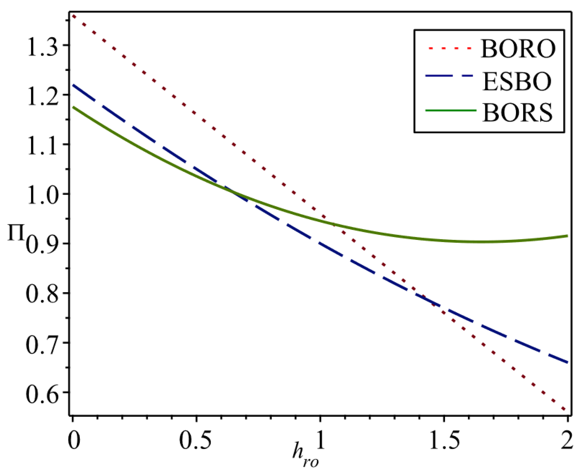
Figure 7 shows comparisons of the changes in retailer profits as return transportation costs change. Firstly, the ESBO and BORS omni-channel strategies are compared with the BORO single-channel strategy to show when it is beneficial to open offline stores through comparative analyses. As can be seen from the figure, as return transportation costs increase, the retailer’s profits gradually decrease with the BORO and ESBO strategies, while the retailer’s profits first decrease and then slowly increase with the BORS strategy. It can be seen that return transportation costs have a smaller impact on retailers that allow consumers to return products offline. Comparing the retailer’s profits in the case of whether or not it set up an experience store or a physical store, we can see that the retailer sets lower return penalties when it has lower return transportation costs. Therefore, consumers prefer online shopping to visiting an experience store or a physical store. The retailer has no incentive to open offline showrooms beyond the existing online channel. On the other hand, the retailer sets higher return penalties when it has higher return transportation costs. As a result, some consumers choose not to purchase from the online channel. The retailer builds offline experience stores or physical stores to attract these consumers, reducing returns and increasing profits by reducing consumer uncertainty about product matching.

We comprehensively compare the impact of the unit return transportation cost on the retailer’s profits when using three channel strategies. It can be seen that when the unit return transportation cost is low, the profit of adopting the BORO strategy is higher than that of the other two strategies. As a result, the retailer tends to sell its products only through the online channel and has no incentive to open offline channels. This can explain why retailers with efficient logistics systems do not open offline channels. Many apparel retailers on e-commerce platforms have built long-term strategic partnerships with upstream manufacturers and large downstream logistics companies. As a result, they have lower return costs and can improve their profitability. As the online return transportation cost per unit of product increases, retailers may increase the price of their products to compensate for the increase in costs. They may also increase the return penalties. These actions will cause consumers to make fewer online returns. As a result, because of the increased cost of online returns, some consumers will buy fewer products, which, in turn, adversely affects retailers’ profits. In order to prevent the decrease in profit, retailers will choose to open offline channels to reduce online returns. When the return transportation cost per unit of product is high, retailers choose to open offline physical stores as the best channel. In addition, it can be seen that the BORS strategy is least affected by the return transportation costs, as it can offer returns from offline channels. This allows the strategy to reduce the negative impact of increased online return transportation costs.

5.1.2. The Impact of Online Return Hassle Cost on the Retailer’s Profits

Figure 8 shows comparisons of the changes in retailer profits as online return hassle costs change. First, the ESBO and BORS omni-channel strategies are compared with the BORO single-channel strategy, to show when it is beneficial to open offline stores through a comparative analysis. As can be seen in the figure, as online return hassle costs increase, retailer profits gradually decrease with the BORO and ESBO strategies, while retailer profits first decrease and then slowly increase with the BORS strategy. Moreover, the BORO strategy outperforms the ESBO strategy and the BORS strategy at smaller values of $h_{ro}$. Obviously, lower online return hassle costs make it easier for consumers to buy and return products online. As the online return hassle cost increases, many consumers no longer choose to buy online. In order to increase their profits, retailers open offline experience stores or physical stores, incentivizing consumers to buy after the experience at the experience stores or directly at the physical stores. This reduces the retailer’s loss of profits due to the inconvenience of consumers’ returns. At the same time, if retailers want to drive traffic to offline channels, they can increase sales in offline experience stores or physical stores by increasing the online return hassle cost. Thus, retailers can profit from targeted segment channels.

For consumers, the online return hassle cost is an important factor influencing online purchases, and it plays an important role in determining the optimal channel strategy for retailers. Comparing the three models, we can see that the BORO strategy outperforms the other two strategies when the online return hassle cost is low. This is intuitive because lower online return hassle costs make it more convenient for consumers to buy online. As the online return hassle cost increases, retailers are more likely to choose to open offline physical stores. For example, the Japanese brand Uniqlo has established a large number of offline physical stores to provide consumers with purchase and return services. Furthermore, it is found that the BORS channel is the least sensitive to online return hassle costs. This is also due to the fact that offline physical stores can provide consumers with additional purchase and return channels, which are less affected by online return hassle costs.

5.1.3. The Impact of Retail Price on the Retailer’s Profits

Figure 9 presents comparisons of the changes in retailer profits as the retail price changes. As can be seen from the figure, with all three strategies, retailer profits show a tendency to increase and then decrease as the price increases. This is reasonable because with the BORO strategy, the initial increase in price is within the range of consumers’ acceptance, and the profits grow as the price increases. However, when the price is too high, online consumers are more price-sensitive and purchase less, resulting in a decrease in total profits. Moreover, online competition is fierce, and prices that are too high tend to make consumers turn to other merchants. With the ESBO strategy, consumers have a more intuitive understanding of the products through offline experiences and are willing to accept a certain price increase, so profits rise in the early stage. After the price reaches a certain level, even with the advantages of offline experience, the high price still inhibits the demand, and profits began to decline. With the BORS strategy, the price increase in the early period brings rapid growth in profits. Since the convenience of offline returns attracts consumers, retailers are able to maintain the sales even at slightly higher prices. The combination of consumers’ reduced willingness to buy when prices are too high and the fact that allowing offline returns increases the retailer’s offline processing costs leads to a gradual decline in profits.

Comprehensively comparing the impact of retail price on the retailer’s profits when using the three channel strategies, we can see that the strategy of opening physical stores is significantly more profitable for the retailer than the other two strategies are. Obviously, in the BORS model, allowing returns to physical stores greatly reduces the risk of shopping for consumers. They do not have to worry about the difficulty of returning unsuitable products, which greatly enhances their willingness to buy. The returned products can be quickly re-entered into the offline inventory, speeding up the inventory turnover and reducing the backlog costs. In addition, the ESBO strategy is more profitable than the BORO strategy for the retailer. Consumers who experience the products offline have a better idea of whether the products meet their needs. They make more rational purchasing decisions, with fewer returns due to information asymmetry. Even if the price is slightly higher online, they are more willing to buy.

5.2. Numerical Analysis

5.2.1. The Impact of the Fashion Level Existence Time on the Retailer’s Profits

The fashion level existence time denotes the process that fashionable clothing undergoes from the moment it is put on the shelves until its fashion level decays to zero, which is commonly known as the time of the “season’s new arrivals”. The fashion level of clothing affects sales and, therefore, the retailer’s profits during the selling period.

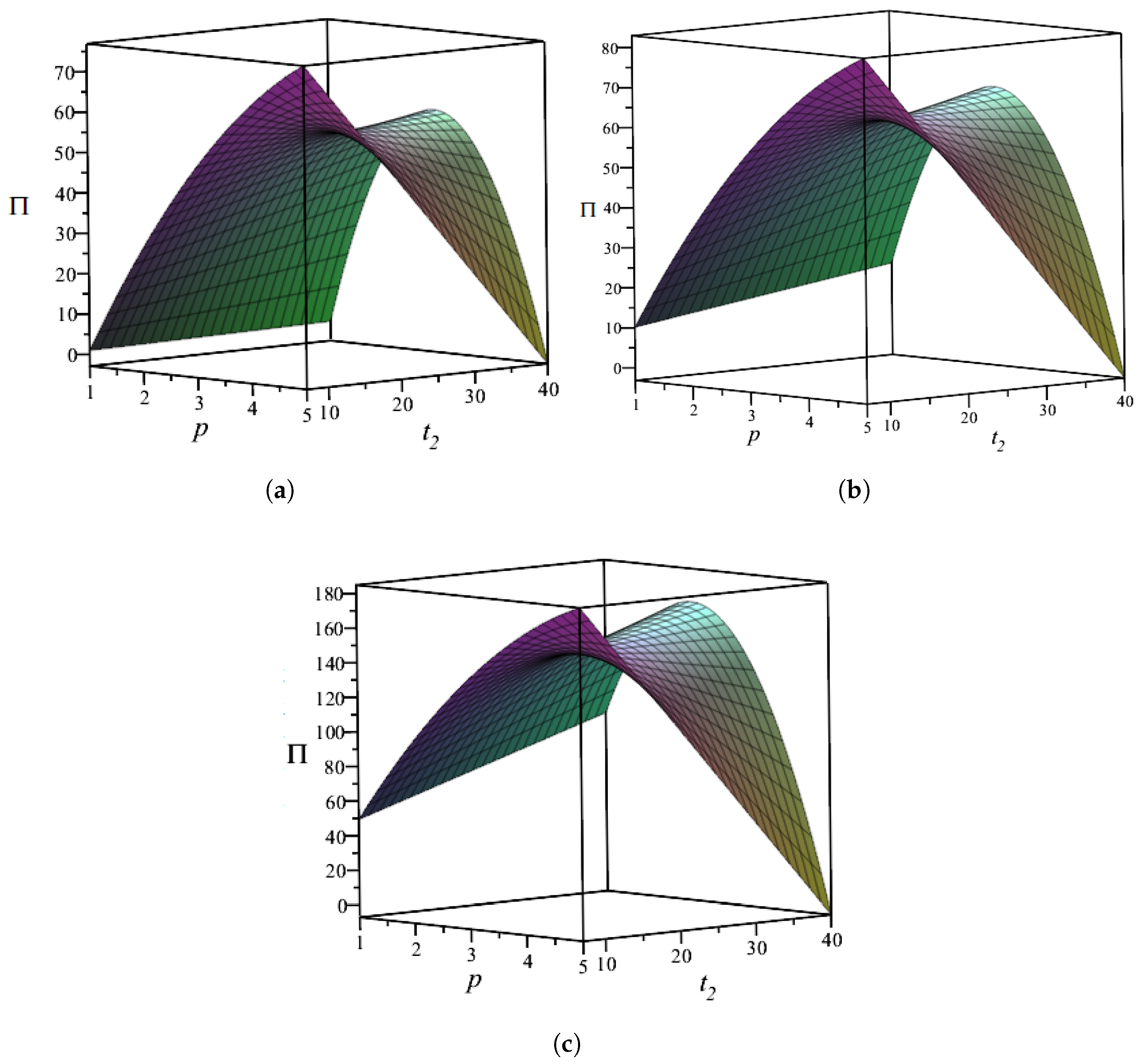
As can be seen in Figure 10, the effect of price and fashion level existence time $t_1$ on the retailer’s profit is positive. At the optimal retail price, the retailer’s profit increases as $t_1$ increases. However, after $t_1$ increases to a certain value, the positive effect on profit diminishes. In practice, it is effective for retailers to maintain a certain fashion level existence time. Retailers who maintain the fashion level for a certain period of time are able to increase the sales generated by the fashion level of apparel and attract consumers to buy during this period of time. However, after $t_1$ reaches a certain value, continuing to extend the fashion level existence time may not increase the retailer’s profit because of the gradual increase in the costs. The retailer may have to continue to invest in advertising costs in order to continue to attract consumers, which may not have a significant effect on the increase in profit.

In addition, it can be seen that the relationships between the retailer’s profits at the same retail price and the fashion level existence time when using the three strategies are as follows. The profit is the lowest with the BORO strategy. The ESBO strategy can provide more profit than the BORO strategy. The profit with the BORS strategy is higher than the profit with the ESBO strategy. Profits will be increased to some extent by the BORS strategy since it offers an extra offline channel for consumers who prefer the offline channel over the ESBO strategy.

5.2.2. The Impact of Continuing Sales Time on the Retailer’s Profits

Continuing sales time denotes the period from when the fashion level of fashionable clothing decays to zero until the clothing’s removal from the shelves. During this time, fashionable garments become outdated and out of style, losing their fashion value. Retailers usually sell them at a discount and remove them from the shelves after a certain period of time.

As can be seen in Figure 11, the impact of price and continuing sales time $t_2$ on retailers’ profits presents a relatively complex change. When the retail price is low, the retailer’s profit gradually increases as the continuing sales time $t_2$ increases. However, when the retail price increases to a certain value, the retailer’s profit gradually decreases with the increase in the continuing sales time $t_2$. For fashionable clothing with relatively low retail prices, retailers can increase profits by increasing the continuing sales time. However, for fashionable clothing with relatively high prices, after the fashion level declines to zero, blindly extending the sales time reduces profits. This can provide good theoretical support for the sales phenomenon of fashionable clothing with high prices. Generally, the sales period of high-end fashionable clothing is controlled within a relatively short period, and retailers use this method to ensure the high-end fashion brand effect of their own clothing.

We compare the BORO strategy, the ESBO strategy, and the BORS strategy. When the pricing is lower, the sensitivity of retailers’ profits to continuing sales time increases in the order of the BORO strategy, the ESBO strategy, and the BORS strategy. That is to say, at the same price, the retailer’s profit in the BORS strategy increases more significantly with the increase in the continuing sales time. In other words, opening offline physical stores is more advantageous for extending the sales time of lower-priced fashionable clothing, followed by the opening of experience stores. This can be explained by the fact that retailers opening physical stores or experience stores have an advantage over single-channel online retailers. They provide consumers with a channel for offline exposure to products. In addition, extending the sales time can provide consumers with more opportunities for exposure. Comparing experience stores and physical stores, we find that fashionable clothing will continue to be sold as regular clothing in physical stores after the fashion level decays to zero. However, at this time, experience stores take out-of-date clothes off the shelves one after another. As a result, the effect of the increase in the continuing sales time on the profit of experience stores is smaller than that of physical stores.

5.2.3. The Impact of the Initial Fashion Level on the Retailer’s Profits

The initial fashion level indicates the fashion level of a fashionable garment at the time of its launch, and it represents the initial level of trendiness assigned to the apparel by retailers. The initial fashion level is usually determined during the design stage. The marketing strategy when products are put on shelves affects how well the initial fashion level is received by consumers. It reflects retailers’ efforts to make products fashionable at launch.

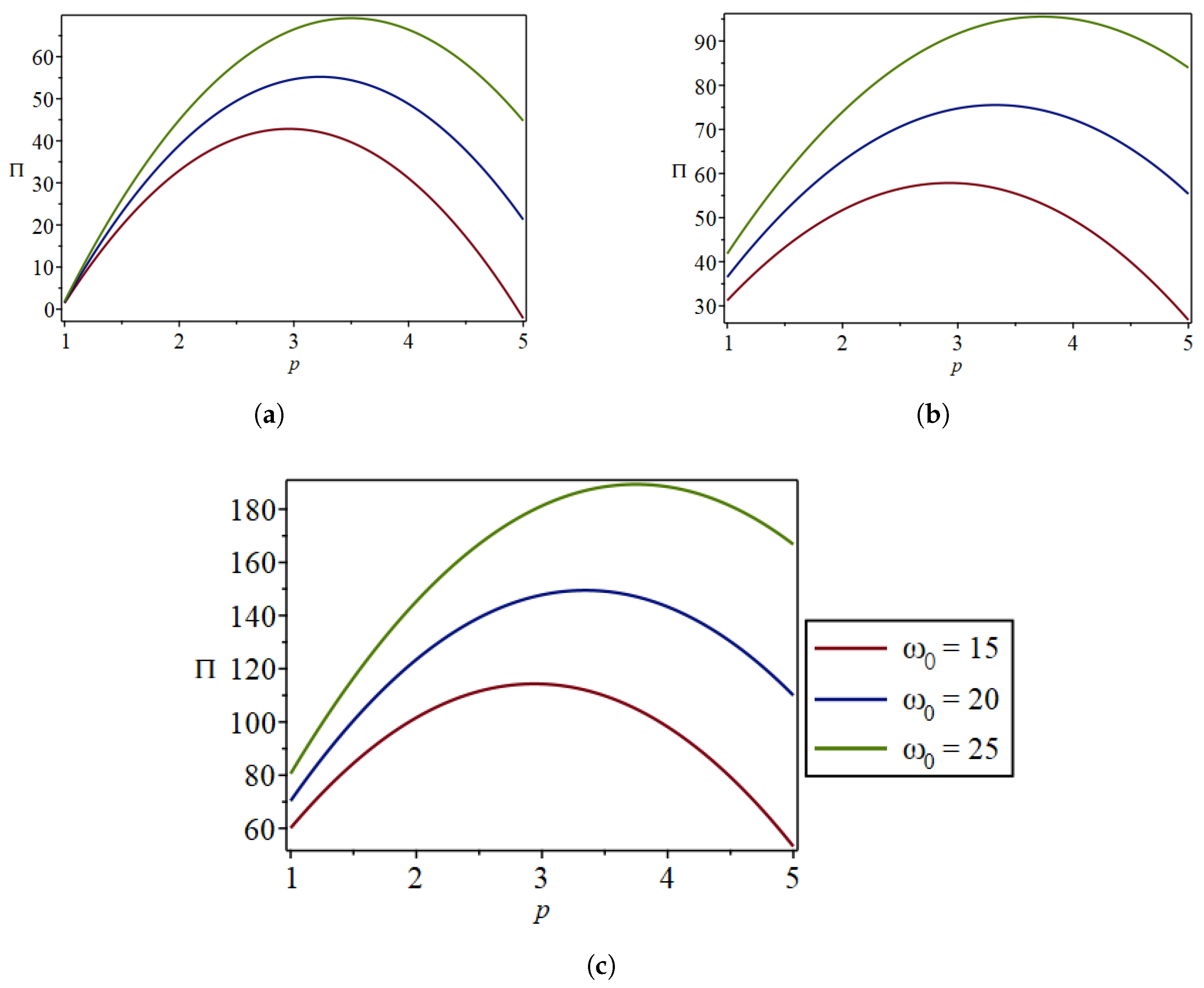
As can be seen in Figure 12, as the initial fashion level increases, the optimal profit of retailers at the same retail price gradually increases. Under the same conditions, the greater the initial fashion level, the longer the fashion level existence time, which will bring greater profits to retailers. In real business, before or at the initial stage of the clothing market, retailers use some marketing methods to increase the initial fashion level of clothing to improve the profit during the entire sales period. It is worth noting that in the three strategies, the greater the initial fashion level, the greater the optimal retail price. That is, for clothing with a relatively high initial fashion level, retailers can achieve the maximum profit by appropriately increasing the retail price. A larger initial fashion level means a longer fashion level existence time and that consumers have more access to the products. It also means that consumers have a higher price acceptance for more fashionable products. Retailers can increase their profits through appropriately increasing the retail price.

In addition, it can be seen that there are significant differences between the ESBO strategy, the BORS strategy, and the BORO strategy. The difference is that the distance between the three curves is greater. In other words, the profit change brought by changing the initial fashion level in the ESBO strategy and the BORS strategy is more significant. This indicates that when opening a showroom for omni-channel operation, the retailer should pay more attention to the initial fashion level of fashionable clothing. Increasing the initial fashion level can bring more obvious benefits in terms of profits. For clothing with a high initial fashion level, a showroom can provide consumers with opportunities to touch and feel fashionable clothing, leading to greater recognition of the fashion level. As a result, this enhances consumer willingness and brings more profit to retailers.

5.2.4. The Impact of the Fashion Level Decay Factor on the Retailer’s Profits

The fashion level decay factor indicates how quickly the fashion level of apparel changes over time. It describes the phenomenon of fashion level decay over the duration of the fashion level existence time. The larger the fashion level decay factor, the faster the fashion level decays. This reflects the fact that fashionable garments are not recognized as trendy in the market.

As can be seen in Figure 13, with the increase in the fashion level decay factor, the optimal profit of retailers at the same retail price gradually decreases. The larger the fashion level decay factor, the faster the fashion level decays, resulting in reduced demand and lower profits. The fast decay of the fashion level corresponds to a short fashion level existence time. According to the analysis in Section 5.2.1, in the case of a shorter fashion level existence time, increasing the fashion level existence time has a more significant effect on improving profits. This is consistent with the conclusion of this section. It is worth noting that the larger the fashion level decay factor, the smaller the optimal retail price; that is, for fashionable clothing with fast fashion level attenuation, retailers need to establish relatively low retail prices in order to achieve the maximum profit. It is reasonable for retailers to attract more consumers to make purchases through lower pricing when launching fashionable clothing with a fast fashion level decay. It can also be seen from the figure that apparel retailers with a lower fashion level decay factor benefit more. However, if the price of products is set too high, the demand will decrease significantly, and they will not be as profitable as apparel retailers with a higher fashion level decay factor. It can also be seen that the BORS strategy is the best choice for either type of fashionable apparel retailer.

Similarly, one significant difference in the ESBO strategy, the BORS strategy, and the BORO strategy is that the distance between the three curves is greater. In other words, the profit change brought by changing the fashion level decay factor in the ESBO strategy and the BORS strategy is more significant. This indicates that, when opening a showroom for omni-channel operation, retailers should pay more attention to the changes in the fashion level decay factor of fashionable clothing. Reducing the decay factor can bring more obvious benefits in terms of profits.

6. Conclusions and Future Research

6.1. Conclusions

This work focused on omni-channel retailing. It constructed and analyzed a BORO single-channel model, an ESBO omni-channel model with experience stores, and a BORS omni-channel model with physical stores, with the aim of solving problems relating to retailing and returns in the apparel industry. The study analyzed the pricing and return decisions of a retailer when using the three strategies. Subsequently, it analyzed the pricing and return strategies of the retailer with two different types of showroom models while considering the influence of the fashion level decay factor. Then, a sensitivity analysis and numerical analysis of important parameters were performed. Our research yielded the following conclusions.

Firstly, this work demonstrated that opening an offline store is not always favorable, and it requires certain conditions. As return transportation costs and online return hassle costs increase, the retailer’s profits when using the BORO and ESBO strategies decrease, while the retailer’s profits when using the BORS strategy first decrease and then slowly increase. It can be seen that the costs associated with online returns have a smaller impact on retailers who allow consumers to return products offline. Moreover, the retailer’s profits in the BORS channel are the least sensitive to online return hassle costs, and their profits in the BORO channel are the most sensitive to online return hassle costs. Therefore, retailers with a BORO strategy should be more concerned about the impact of online return hassle costs. The three strategies were compared horizontally: (1) when the retailer has a lower return transportation cost, they set a lower return penalty, and consumers prefer direct online shopping. Thus, the retailer has no incentive to open a showroom. When the retailer’s return transportation cost is high, they will set a higher return penalty. The retailer can establish an experience store or a physical store to attract consumers, thereby reducing the uncertainty of product matching to reduce returns and increase profits. The BORS strategy is the optimal option for the retailer. (2) When the online return hassle cost is low, consumers’ online purchases and returns are more convenient, and the BORO strategy outperforms the ESBO strategy and the BORS strategy. However, with an increase in the online return hassle cost, consumers no longer choose to purchase online due to the inconvenience of returning products. The retailer can encourage consumers to purchase after experiencing products in a showroom through opening an offline experience store or to purchase directly by opening an offline physical store, thereby improving profits. The BORS strategy outperforms the ESBO strategy when the online return hassle cost is higher, reflecting one of the major advantages for retailers in opening physical stores for consumer purchases and returns with the BORS strategy. In addition, this study also revealed that, with the three strategies, the retailer’s profits increase and then decrease with increasing retail price when all other conditions are equal. Changes in retail price have the greatest impact on retailer profits when using the BORS strategy. Therefore, retailers who add physical stores should pay more attention to the setting of the retail price.

Secondly, changes in the selling period of fashionable apparel were found to have an important impact on the retailer’s profits when using the three strategies. The selling period of apparel affects sales and retailer profits. The effect of the fashion level existence time on the retailer’s profits is positive. At the optimal retail price, the retailer’s profit increases as the fashion level existence time increases. However, its positive effect on profit diminishes after the fashion level existence time increases to a certain value. Retailers maintaining a certain fashion level existence time can be effective in increasing sales. However, excessive extension of the fashion level existence time may require retailers to incur more marketing costs, which is detrimental to the total profitability. When the retail price and fashion level existence time are the same, the retailer’s profits are the lowest when using the BORO strategy and the highest when using the BORS strategy. The BORS strategy increases the profits, to some extent, as it adds an additional offline purchasing channel with respect to the ESBO strategy. In addition, when the retail price is low, the retailer’s profit gradually increases as the continuing sales time increases. However, after the retail price increases to a certain value, the retailer’s profit gradually decreases as the continuing sales time increases. For fast-fashion clothing with lower retail prices, retailers can increase their profits through increasing the continuing sales time. The strategy of opening offline physical stores is the most favorable for extending the selling time for fast-fashion garments, followed by the strategy of opening experience stores. However, the selling period of high-end fashionable apparel (e.g., luxury apparel) is controlled in a shorter period to ensure the high-end fashion brand effect of the apparel. In summary, different fashionable apparel retailers can maximize their profits by determining the selling time period rationally.

Thirdly, the fashion level decay factor was found to have a significant impact on the retailer’s profits when using the three strategies. The fashion level first affects the retailer’s optimal pricing. The fashion level is also controlled by the retailer through some links such as design and marketing, such that the optimal retail price can be determined. The retailer can also dynamically adjust the price during the selling period for different sales purposes; for example, after fashionable clothing is converted into general clothing, the retailer can promote the products by reducing the price. As the initial fashion level increases, the retailer’s optimal profit at the same retail price gradually increases. For garments that are initially more fashionable, retailers can maximize their profits by increasing the retail price appropriately. In addition, as the fashion level decay factor increases, the retailer’s optimal profit at the same retail price gradually decreases. For fast-fashion apparel with a fast fashion level decay, retailers have to set relatively low retail prices to maximize profits. To the contrary, for luxury apparel with a slow fashion level decay, consumers can accept higher retail prices set by retailers. Overall, luxury apparel retailers benefit more. However, if the price of the products is too high, the demand will be much lower, and it will not be as profitable as it is for fast-fashion apparel retailers. It can also be found that the BORS strategy is the best option for both types of fashionable apparel retailers. In actual operation, before or at the early stage of the launch of garments, retailers can increase the initial fashion level of garments through adding fashionable design elements and some marketing means. They can also reduce the fashion level decay factor to increase the profit in the whole sales period through corresponding marketing means. In particular, the impact of changes in the fashion level on changes in the retailer’s profits is more pronounced under the ESBO and BORS strategies. Retailers with offline experiential and physical stores need to focus more on increasing the initial fashion level and decreasing the fashion level decay factor, which is also a challenge for retailers with omni-channel operations. This is because, if retailers fail to maintain the fashion level, the negative impact on their profits will also increase. Furthermore, fashionable apparel retailers that add offline stores have to be careful to weigh the negative impacts of operating and marketing costs on their profitability. This is also a challenge that omni-channel retailers have to face.

6.2. Managerial Implications

Our findings have the following implications for management research.

Firstly, retailers should choose whether or not to open offline channels based on their own circumstances. If they do, they should choose the format of their offline stores (experience stores or physical stores) carefully. When faced with consumer returns, opening an offline channel may decrease retailers’ profits if they have lower return transportation costs. However, it is undeniable that more and more apparel retailers are leaning towards omni-channel operations as they need to expand the range of consumers that they serve. Lower online return hassle costs are more favorable for consumers to make online purchases and returns. However, to some extent, this is in conflict with retailers’ desire to reduce return rates. The previous analysis showed that lower online return hassle costs are beneficial for online channel operations. Retailers can reduce the return transportation costs using certain methods, such as establishing long-term cooperations with professional third-party logistics enterprises to reduce the transportation costs borne in the return process. Further, if retailers wish to reduce returns by raising online hassle costs, they face the risk of a shrinking market share; therefore, they should reasonably assess this risk. When retailers try to decrease consumer returns by raising the online return hassle costs, they may choose to open offline stores to face the risk of shrinking market shares. Offline stores can provide offline services to consumers who are reluctant to make purchases due to the hassle of online returns, reducing the return rate while avoiding a significant loss in turnover.

Secondly, the omni-channel retail management of fashionable clothing is complex. Due to the rapid changes in demand, retailers need to make more efforts to increase profits. It is obvious that extending the sales time of fashionable clothing has a positive effect on profits, but blindly increasing the sales time of fashionable clothing is not always beneficial. During the sales period of the fashion level existence time, retailers may incur greater costs to extend the fashion level existence time of fashionable apparel, such as continuous advertising. When the cost incurred exceeds the revenue generated from sales, retailers should transform fashionable clothing into general style clothing for processing. Similarly, after the fashion level declines to zero, blindly extending the sales time would lead to a decrease in profits. Especially for high-end fashionable clothing with higher prices, retailers generally control the sales period for a relatively short time. They may even immediately remove such clothing from the shelves after the fashion level fades to zero. Many retailers use this method to ensure the high-end fashion brand effect.

Thirdly, the fashion level decays over time. The fashion level decay factor and initial fashion level are relatively abstract concepts, indicating a level of effort by retailers to create fashionable clothing. The initial fashion level of clothing should be improved during design, and the rate of decline in the fashion level should be slowed down through marketing efforts during the sales period. Through analysis, it was found that a larger fashion level decay factor means that the fashion level decays faster and the optimal profit decreases. In addition, the larger the fashion level decay factor, the smaller the optimal retail price; that is, for fashionable clothing with a fast fashion level decay, retailers need to set relatively low retail prices in order to achieve maximum profit. Under the same conditions, the higher the initial fashion level, the longer the fashion level existence time, which will bring greater profits to retailers. Similarly, it can be observed that the higher the initial fashion level, the higher the optimal retail price. Consumers increase their acceptance of prices due to high initial fashion levels. In this case, retailers can achieve maximum profits through appropriately increasing their retail prices.

6.3. Future Research

This article focuses on omni-channel strategies considering returns under the influence of fashion level decay, and provides practical guidance for retailers’ omni-channel operation. However, the article has some limitations at the same time. In future studies, we can research the following aspects to further improve research in related fields.

Firstly, we can conduct research on other omni-channel retail operation models and other fashion level decay models, while this article focused on omni-channel strategy choices for experience stores and physical stores, there are also different omni-channel operation and delivery models, such as “Buy Online and Pick up in Store (BOPS)” [67]. In future research, we can continue to establish models according to the research ideas of this article for different operation models, supplementing the research on several omni-channel models in the field of clothing retail. In addition, in terms of fashion level decay, the common exponential decay model was chosen in this article. In future research, the impacts of other decay models (e.g., the polynomial decay model and stepwise decay model) on the profitability of apparel retailers can be discussed and compared.

Secondly, consumers should be segmented. Consumers have significant differences. In future research, we can further classify consumer types. Many studies classify and analyze consumers based on their different characteristics, exploring the impacts of consumers with different channel preferences and levels of cost sensitivity [68] on the results. In future research, we can focus on heterogeneous consumers and further segment them. For example, we can classify consumers based on their loyalty to online and offline channels. We can also study the impacts of different types of consumers on omni-channel retail and help retailers make correct decisions when facing different consumer groups.

Thirdly, fashionable apparel retailers’ dynamic pricing and the profit distribution issue behind cross-channel returns are also valuable research directions in the future. Although we considered pricing decisions in our models, these are not affected by time. In reality, fashion retailers often engage in dynamic pricing. Therefore, dynamic pricing strategies (e.g., markdown strategies and seasonal price adjustments) for fashionable apparel are a worthwhile direction to explore in the future. In addition, omni-channel operations integrate the previously fragmented online and offline channels. It is very important for retailers to allocate the income, profits, and costs generated in omni-channel operations. In the future, we can explore how to design effective profit-sharing mechanisms to incentivize retailers to adopt more effective return strategies and further research the problem of allocation between channels.

Fourthly, empirical research should be conducted. This article focused on the in-depth exploration of theoretical models using mathematical modeling. In the future, valuable empirical research can be conducted on the pricing and return issues of fashionable apparel retailers. We can use empirical data to conduct an in-depth validation and detailed analysis of the model. This will not only provide a solid empirical basis for the operation of the fashionable apparel retail sector, but is also expected to open up new paths for practical applications in the fashionable apparel industry.