A Fractional Adams Method for Caputo Fractional Differential Equations with Modified Graded Meshes

Abstract

In this paper, we introduce an Adams-type predictor–corrector method based on a modified graded mesh for solving Caputo fractional differential equations. This method not only effectively handles the weak singularity near the initial point but also reduces errors associated with large intervals in traditional graded meshes. We prove the error estimates in detail for both $0<\alpha <1$ and $1<\alpha <2$ cases, where $\alpha$ is the order of the Caputo fractional derivative. Numerical experiments confirm the convergence of the proposed method and compare its performance with the traditional graded mesh approach.

1. Introduction

In this paper, we introduce a fractional Adams method with a modified graded mesh for solving the following nonlinear fractional differential equation, with $0<\alpha <2$:

$$\begin{array}{cc}\hfill & {}_0{}^{C}D_t^{\alpha }u\left(t\right)=g(t,u\left(t\right)),t>0,\hfill \\ \hfill & u^{\left(k\right)}\left(0\right)=u_0^{\left(k\right)},k=0,1,\dots ,\lceil \alpha \rceil -1,\hfill \end{array}$$

(1)

where $u_0^{\left(k\right)}$ are arbitrary real numbers and ${}_0{}^{C}D_t^{\alpha }u\left(t\right)$ represents the Caputo fractional derivative, defined by:

$${}_0{}^{C}D_t^{\alpha }u\left(t\right)={\displaystyle \frac{1}{\Gamma (\lceil \alpha \rceil -\alpha )}}{\int }_0^t{(t-s)}^{\lceil \alpha \rceil -\alpha -1}{u}^{(\lceil \alpha \rceil )}\left(s\right)ds,$$

(2)

with $\Gamma (·)$ denoting the Gamma function and $\lceil \alpha \rceil$ representing the smallest integer greater than or equal to $\alpha$. The function $g(t,u)$ satisfies the Lipschitz condition with respect to the second variable, i.e.,

$$|g(t,u_1)-g(t,u_2)|\le L|u_1-u_2|,u_1,u_2\in \mathbb{R},$$

where L is a positive constant.

We shall focus only on the case $0<\alpha <2$, as $\alpha >2$ does not appear to be of significant practical interest ([1], lines 4–5 on page 46). The error estimates for the case $\alpha >2$ can be derived in a similar manner.

It is well-known that Equation (1) is equivalent to the following integral representation:

$$u\left(t\right)={\displaystyle \sum _{\nu =0}^{\lceil \alpha \rceil -1}}{u}_0^{\left(\nu \right)}{\displaystyle \frac{t^{\nu }}{\nu !}}+{\displaystyle \frac{1}{\Gamma \left(\alpha \right)}}{\int }_0^t{(t-s)}^{\alpha -1}g(s,u\left(s\right))ds.$$

(3)

The existence and uniqueness of the solution to Equation (1) have been thoroughly discussed in [1].

The numerical solution of fractional differential equations (FDEs) has been a topic of significant research interest in recent decades due to their applications in fields such as physics, biology, and engineering [2,3]. Exact solutions for FDEs are often difficult to obtain. Therefore, it is necessary to develop some efficient numerical methods for solving FDEs.

In addition to Adams methods, other numerical techniques for solving FDEs have been extensively explored. One approach involves directly approximating the fractional derivative, as discussed in [4,5,6]. Another transforms the FDEs into equivalent integral forms, which are then solved using quadrature-based schemes [7,8,9,10,11,12,13]. Furthermore, alternative strategies, such as variational iteration [14], Adomian decomposition [15], finite-element [16], and spectral methods [17], have been developed to address specific FDEs.

The Adams methods, particularly the predictor–corrector variants, have received significant attention for their efficiency in solving FDEs. For instance, Deng [18] enhanced the Adams-type predictor–corrector method by incorporating the short memory principle of fractional calculus, thereby reducing computational complexity. Nguyen and Jang [19] introduced a new prediction stage with the same accuracy order as the correction stage, while Zhou et al. [20] developed a fast second-order Adams method on graded meshes to solve nonlinear time-fractional equations, such as the Benjamin–Bona–Mahony–Burgers equation. Moreover, Lee et al. [21] and Mokhtarnezhadazar [22] proposed an efficient predictor–corrector method based on the Caputo–Fabrizio derivative and a high-order method on non-uniform meshes, respectively. These advancements help reduce computational effort while maintaining high precision.

Among the many numerical methods available for solving FDEs, Diethelm et al. [1,23,24,25] provided the theoretical foundation for the fractional Adams method. They proposed an Adams-type predictor–corrector scheme on uniform meshes and provided rigorous error estimates under the assumption that $g\left(t\right):={}_0{}^{C}D_t^{\alpha }u\left(t\right)\in C^2[0,T]$. The method achieves convergence rates of $O\left(N^{-(1+\alpha )}\right)$ for $0<\alpha \le 1$ and $O\left(N^{-2}\right)$ for $\alpha >1$, where N is the number of the nodes of the time partition on $[0,T]$. These results have since inspired various extensions and refinements. Liu et al. [26] introduced graded meshes to better handle the singular behavior of solutions near $t=0$. Their analysis refined error estimates and demonstrated that graded meshes significantly improve accuracy for FDEs with initial singularities, making them a practical choice for challenging problems. Furthermore, fractional calculus is more flexible than classical calculus, and recently, some new fractional definitions have been developed (see [27]). These developments provide new perspectives and tools for the numerical solution of fractional differential equations.

In this paper, we propose a modified Adams-type predictor–corrector method with a modified graded mesh. This type of mesh was first introduced in [28]. The modified graded mesh employs a non-uniform grid near the initial point to capture weak singularities, while a uniform grid is used away from the initial point, effectively reducing numerical errors. Our approach not only preserves the advantages of traditional graded meshes but also further optimizes the grid distribution, improving the accuracy of the numerical solutions.

Let $0=t_0<t_1<t_2<\cdots <t_N=T$ be a partition; we shall consider the following modified graded mesh [28]. Define $\overline{M}\left(t\right)$ as a positive monitor function:

$$\overline{M}\left(t\right)=max\left\{T,K{t}^{{\displaystyle \frac{\alpha }{2}}-1}\right\},$$

where $K\in (0,T]$ is a constant and $0<\alpha <2$. The mesh is constructed such that $\overline{M}\left(t\right)$ is evenly distributed, i.e.,

$${\int }_{t_n}^{t_{n+1}}\overline{M}\left(s\right)ds={\displaystyle \frac{1}{N}}{\int }_0^T\overline{M}\left(s\right)ds,\mathrm{for}n=0,1,\dots ,N-1.$$

Define $\overline{\sigma }={\left({\displaystyle \frac{T}{K}}\right)}^{{\displaystyle \frac{2}{\alpha -2}}}$ and choose a suitable $K\in (0,T]$ such that $t_J=\overline{\sigma }$ for some $J\le N$. The modified graded mesh ${\left\{t_n\right\}}_{n=0}^N$ is defined as follows:

$$t_n=\left\{\begin{array}{cc}{\left({\displaystyle \frac{\alpha Pn}{2KN}}\right)}^{{\displaystyle \frac{2}{\alpha }}},\hfill & n=0,1,\cdots ,J-1,\hfill \\ \left(1-{\displaystyle \frac{2}{\alpha }}\right)\overline{\sigma }+{\displaystyle \frac{Pn}{TN}},\hfill & n=J,J+1,\cdots ,N,\hfill \end{array}\right.$$

(4)

where $P=T^2+T\overline{\sigma }\left({\displaystyle \frac{2}{\alpha }}-1\right)$. The grid points $\{t_n\mid n=0,1,\dots ,J-1\}$ constitute a non-uniform grid, whereas the grid points $\{t_n\mid n=J,J+1,\dots ,N\}$ form a uniform grid [28].

Let $u_k\approx u\left(t_k\right)$ for $k=0,1,2,\dots ,n+1$, with $n=0,1,2,\dots ,N-1$ being the approximation of $u\left(t_k\right)$. Suppose we know the approximate values $u_0$, $u_1$ from other methods. For $n\ge 2$, we define the following predictor–corrector Adams method to solve Equation (3) for $\alpha \in (0,2)$:

$$\begin{array}{cc}\hfill u_{n+1}^P& ={\displaystyle \sum _{\nu =0}^{\lceil \alpha \rceil -1}}{u}_0^{\left(\nu \right)}{\displaystyle \frac{t_{n+1}}{\nu !}}+{\displaystyle \frac{1}{\Gamma \left(\alpha \right)}}{\displaystyle \sum _{k=0}^n}{p}_{k,n+1}g(t_k,u_k),\hfill \end{array}$$

(5)

$$\begin{array}{cc}\hfill u_{n+1}& ={\displaystyle \sum _{\nu =0}^{\lceil \alpha \rceil -1}}{u}_0^{\left(\nu \right)}{\displaystyle \frac{t_{n+1}}{\nu !}}+{\displaystyle \frac{1}{\Gamma \left(\alpha \right)}}\left({\displaystyle \sum _{k=0}^n}{q}_{k,n+1}g(t_k,u_k)+q_{n+1,n+1}g(t_{n+1},u_{n+1}^P)\right).\hfill \end{array}$$

(6)

The predictor term $u_{n+1}^P$ in (5) is derived by approximating the integral $n\ge 2$,

$${\int }_0^{t_{n+1}}{(t_{n+1}-s)}^{\alpha -1}g(s,u\left(s\right))ds,$$

with the following approximation, $n\ge 2$,

$${\int }_0^{t_{n+1}}{(t_{n+1}-s)}^{\alpha -1}{P}_0\left(s\right)ds,$$

where $P_0\left(s\right)$ is a piecewise constant function defined on $[0,t_{n+1}]$ as, $n\ge 2$,

$$P_0\left(s\right)=g(t_k,u\left(t_k\right)),s\in [t_k,t_{k+1}],k=0,1,2,\dots ,n.$$

The corrector term $u_{n+1}$ in (6) is derived by approximating the same integral, $n\ge 2$,

$${\int }_0^{t_{n+1}}{(t_{n+1}-s)}^{\alpha -1}g(s,u\left(s\right))ds,$$

with the following approximation, $n\ge 2$,

$${\int }_0^{t_{n+1}}{(t_{n+1}-s)}^{\alpha -1}{P}_1\left(s\right)ds,$$

where $P_1\left(s\right)$ is a piecewise linear function defined on $[0,t_{n+1}]$ as, $n\ge 2$,

$$P_1\left(s\right)={\displaystyle \frac{s-t_{k+1}}{t_k-t_{k+1}}}g(t_k,u\left(t_k\right))+{\displaystyle \frac{s-t_k}{t_{k+1}-t_k}}g(t_{k+1},u\left(t_{k+1}\right)),s\in [t_k,t_{k+1}],k=0,1,2,\dots ,n.$$

Here, the weights $p_{k,n+1}$ in (5) for $k=0,1,2,\dots ,n$ are given in Appendix A.

The weights $q_{k,n+1}$ in (6) for $k=0,1,2,\dots ,n+1$, satisfy

$$\begin{array}{c}\hfill q_{k,n+1}=\left\{\begin{array}{cc}{\displaystyle \frac{1}{\alpha (t_1-t_0)}}\left(t_{n+1}^{\alpha }{t}_1+{\displaystyle \frac{1}{\alpha +1}}\left({(t_{n+1}-t_1)}^{\alpha +1}-{(t_{n+1}-t_0)}^{\alpha +1}\right)\right),\hfill & \mathrm{if}k=0,\hfill \\ {\displaystyle \frac{1}{\alpha (\alpha +1)(t_{k-1}-t_k)}}\left({(t_{n+1}-t_k)}^{\alpha +1}-{(t_{n+1}-t_{k-1})}^{\alpha +1}\right)\hfill \\ -{\displaystyle \frac{1}{\alpha (\alpha +1)(t_k-t_{k+1})}}\left({(t_{n+1}-t_{k+1})}^{\alpha +1}-{(t_{n+1}-t_k)}^{\alpha +1}\right),\hfill & \mathrm{if}k=1,2,\dots ,n,\hfill \\ {\displaystyle \frac{1}{\alpha (\alpha +1)}}{(t_{n+1}-t_n)}^{\alpha },\hfill & \mathrm{if}k=n+1.\hfill \end{array}\right.\end{array}$$

(7)

Assumption 1

([26]). Let $0<\sigma <1$ and $f:={}_0{}^{C}D_t^{\alpha }u$ satisfy $f\in C^2(0,T]$ for $\alpha \in (0,2)$. There exists a constant $c>0$ such that:

$$|f^{\prime }\left(t\right)|\le c{t}^{\sigma -1},\left|f^{″}\left(t\right)\right|\le c{t}^{\sigma -2}.$$

Remark 1.

Assumption 1 characterizes the local behavior of $f\left(t\right):={}_0{}^{C}D_t^{\alpha }u$ near $t=0$ and indicates that ${}_0{}^{C}D_t^{\alpha }u$ exhibits a singularity at this point. It is evident that $f\notin C^2[0,T]$. A simple example is $f\left(t\right)=t^{\sigma }$, where $0<\sigma <1$.

Our main results of this work are summarized in the following two theorems.

Theorem 1.

Suppose $0<\alpha <1$ and $f:={}_0{}^{C}D_t^{\alpha }u$ satisfies Assumption 1. Assume that $u\left(t_k\right)$ and $u_k$ are the solutions of Equations (3) and (6), respectively. Then, the following error estimates hold, with $n=2,3,\dots ,N-1$.

1. 

If $t_J\le t_{⌈{\displaystyle \frac{n+1}{2}}⌉-1}$, then we have

$$\underset{0\le k\le n+1}{max}|u\left(t_k\right)-u_k|\le C{N}^{-(\alpha +\sigma )}.$$

2. 

If $t_{\lceil {\displaystyle \frac{n+1}{2}}\rceil }\le t_J\le t_{n+1}$, then we have

$$\underset{0\le k\le n+1}{max}|u\left(t_k\right)-u_k|\le C{N}^{-(\alpha +\sigma )}.$$

3. 

If $t_J>t_{n+1}$, then we have

$$\underset{0\le k\le n+1}{max}|u\left(t_k\right)-u_k|\le \left\{\begin{array}{cc}C{N}^{-r(\alpha +\sigma )},\hfill & \mathit{if}r(\alpha +\sigma )<1+\alpha ,\hfill \\ C{N}^{-(1+\alpha )}lnN,\hfill & \mathit{if}r(\alpha +\sigma )=1+\alpha ,\hfill \\ C{N}^{-(\alpha +1)},\hfill & \mathit{if}r(\alpha +\sigma )>1+\alpha .\hfill \end{array}\right.$$

Theorem 2.

Suppose $1<\alpha <2$ and $f:={}_0{}^{C}D_t^{\alpha }u$ satisfies Assumption 1. Assume that $u\left(t_k\right)$ and $u_k$ are the solutions of Equations (3) and (6), respectively. Then, the following error estimates hold, with $n=2,3,\dots ,N-1$.

1. 

If $t_J\le t_{⌈{\displaystyle \frac{n+1}{2}}⌉-1}$, then we have

$$\underset{0\le k\le n+1}{max}|u\left(t_k\right)-u_k|\le C{N}^{-(1+\alpha )}.$$

2. 

If $t_{\lceil {\displaystyle \frac{n+1}{2}}\rceil }\le t_J\le t_{n+1}$, then we have

$$\underset{0\le k\le n+1}{max}|u\left(t_k\right)-u_k|\le C{N}^{-min\{2,\alpha +\sigma ,r(1+\sigma \left)\right\}}.$$

3. 

If $t_J>t_{n+1}$, then we have

$$\underset{0\le k\le n+1}{max}|u\left(t_k\right)-u_k|\le \left\{\begin{array}{cc}C{N}^{-r(1+\sigma )},\hfill & \mathit{if}r(1+\sigma )<2,\hfill \\ C{N}^{-2}lnN,\hfill & \mathit{if}r(1+\sigma )=2,\hfill \\ C{N}^{-2},\hfill & \mathit{if}r(1+\sigma )>2.\hfill \end{array}\right.$$

The structure of this paper is as follows. In Section 1, we introduce the predictor–corrector method on modified graded meshes for solving Equation (1). Section 2 presents several lemmas for the case $0<\alpha <1$, and Section 3 discusses lemmas for the case $1<\alpha <2$. In Section 4, we provide proofs of the theorems. Section 5 provides numerical examples demonstrating the consistency between the numerical results and the theoretical predictions.

Throughout the paper, the symbol C denotes a generic constant, which may vary across different occurrences but remains independent of the mesh size.

2. Some Lemmas for $\mathbf{0}<\mathbf{\alpha }<\mathbf{1}$

Denote

$$\begin{array}{c}\hfill C_1={\left({\displaystyle \frac{\alpha P}{2K}}\right)}^{{\displaystyle \frac{2}{\alpha }}},C_2=\left(1-{\displaystyle \frac{2}{\alpha }}\right)\overline{\sigma },C_3={\displaystyle \frac{P}{T}},\end{array}$$

(8)

where P, K, $\overline{\sigma }$ are defined in (4). Then, $t_n$ in (4) can be rewritten as follows:

$$t_n=\left\{\begin{array}{cc}{C}_1{\left({\displaystyle \frac{n}{N}}\right)}^r,\hfill & n=0,1,\dots ,J-1,\hfill \\ C_2+C_3\left({\displaystyle \frac{n}{N}}\right),\hfill & n=J,J+1,\dots ,N,\hfill \end{array}\right.$$

where $r={\displaystyle \frac{2}{\alpha }}$, $C_2<0$, $C_3=T-C_2>0$ and J is defined in (4).

Lemma 1.

There exists a positive constant $C_4>0$, such that

$$t_n\ge C_4\left({\displaystyle \frac{n}{N}}\right),n=J,J+1,\dots ,N,$$

where J is defined in (4).

Proof. 

Choose $C_4>0$ such that, since $C_2>0$,

$$1-{\displaystyle \frac{T}{C_2}}+{\displaystyle \frac{C_4}{C_2}}>0.$$

Note that

$${\displaystyle \frac{t_n}{\frac{n}{N}}}={\displaystyle \frac{C_2+C_3\left(\frac{n}{N}\right)}{\frac{n}{N}}}=C_3+{\displaystyle \frac{C_2}{\frac{n}{N}}}=T-C_2+{\displaystyle \frac{N}{n}}{C}_2=C_2({\displaystyle \frac{N}{n}}-1)+T,$$

which implies that when $n>{\displaystyle \frac{N}{1-\frac{T}{C_2}+\frac{C_4}{C_2}}}$, we have

$${\displaystyle \frac{t_n}{\frac{n}{N}}}>C_4.$$

Choose

$$J_1=⌈{\displaystyle \frac{N}{1-\frac{T}{C_2}+\frac{C_4}{C_2}}}⌉,$$

and we see that when $n>J_1$,

$$t_n\ge C_4\left({\displaystyle \frac{n}{N}}\right).$$

Further, we have $J>J_1$. In fact, $t_J=C_2+C_3\left({\displaystyle \frac{J}{N}}\right)$ implies that $J={\displaystyle \frac{(t_J-C_2)N}{C_3}}$. Hence, with $ϵ>0$,

$${\displaystyle \frac{J}{J_1}}\approx {\displaystyle \frac{(t_J-C_2)N}{C_3}}·{\displaystyle \frac{C_2-T+ϵ}{C_{2}N}}={\displaystyle \frac{(t_J-C_2)N}{T-C_2}}·{\displaystyle \frac{C_2-T+ϵ}{C_{2}N}}={\displaystyle \frac{(C_2-t_J)N}{T-C_2}}·{\displaystyle \frac{T-C_2-ϵ}{C_{2}N}}\approx {\displaystyle \frac{C_2-t_J}{C_2}}\ge 1.$$

Thus, for $t_n\ge t_J$, we obtain

$$t_n\ge C_4\left({\displaystyle \frac{n}{N}}\right).$$

The proof of Lemma 1 is complete. □

In the rest of the paper, we assume $J>2$.

Lemma 2.

Suppose $0<\alpha <1$ and $f:={}_0{}^{C}D_t^{\alpha }u$ satisfies Assumption 1. Let $n\ge 2$.

1. 

If $t_J\le t_{⌈{\displaystyle \frac{n+1}{2}}⌉-1}$, then we have

$$\left|{\int }_0^{t_{n+1}}{(t_{n+1}-s)}^{\alpha -1}\left[f\left(s\right)-P_1\left(s\right)\right]ds\right|\le C{N}^{-(\alpha +\sigma )}.$$

2. 

If $t_{\lceil {\displaystyle \frac{n+1}{2}}\rceil }\le t_J\le t_{n+1}$, then we have

$$\left|{\int }_0^{t_{n+1}}{(t_{n+1}-s)}^{\alpha -1}\left[f\left(s\right)-P_1\left(s\right)\right]ds\right|\le C{N}^{-(\alpha +\sigma )}.$$

3. 

If $t_J>t_{n+1}$, then we have

$$\left|{\int }_0^{t_{n+1}}{(t_{n+1}-s)}^{\alpha -1}\left[f\left(s\right)-P_1\left(s\right)\right]ds\right|\le \left\{\begin{array}{cc}C{N}^{-r(\alpha +\sigma )},\hfill & \mathit{if}r(\alpha +\sigma )<2,\hfill \\ C{N}^{-2}lnN,\hfill & \mathit{if}r(\alpha +\sigma )=2,\hfill \\ C{N}^{-2},\hfill & \mathit{if}r(\alpha +\sigma )>2.\hfill \end{array}\right.$$

In the above, $P_1\left(s\right)$ denotes a piecewise linear approximation of $f\left(s\right)$ defined on each interval $[t_k,t_{k+1}]$ for $k=0,1,2,\dots ,n$,

$$P_1\left(s\right)={\displaystyle \frac{s-t_{k+1}}{t_k-t_{k+1}}}f\left(t_k\right)+{\displaystyle \frac{s-t_k}{t_{k+1}-t_k}}f\left(t_{k+1}\right),s\in [t_k,t_{k+1}].$$

Proof. 

For $n=2,3,\dots ,N-1$, we decompose the integral into three parts,

$$\begin{array}{cc}\hfill & {\int }_0^{t_{n+1}}{(t_{n+1}-s)}^{\alpha -1}\left[f\left(s\right)-P_1\left(s\right)\right]ds\hfill \\ \hfill & =\left({\int }_0^{t_1}+{\displaystyle \sum _{k=1}^{n-1}}{\int }_{t_k}^{t_{k+1}}+{\int }_{t_n}^{t_{n+1}}\right){(t_{n+1}-s)}^{\alpha -1}\left[f\left(s\right)-P_1\left(s\right)\right]ds\hfill \\ \hfill & =:H_1+H_2+H_3.\hfill \end{array}$$

Using Assumption 1, we have

$$\begin{array}{cc}\hfill |H_1|& =\left|{\int }_0^{t_1}{(t_{n+1}-s)}^{\alpha -1}\left(f\left(s\right)-{\displaystyle \frac{s-t_1}{t_0-t_1}}f\left(t_0\right)-{\displaystyle \frac{s-t_0}{t_1-t_0}}f\left(t_1\right)\right)ds\right|\hfill \\ \hfill & =\left|{\int }_0^{t_1}{(t_{n+1}-s)}^{\alpha -1}\left(-{\displaystyle \frac{s-t_1}{t_1}}{\int }_0^s{f}^{\prime }\left(\tau \right)d\tau -{\displaystyle \frac{s}{t_1}}{\int }_s^{t_1}{f}^{\prime }\left(\tau \right)d\tau \right)ds\right|\hfill \\ \hfill & \le \left|{\int }_0^{t_1}{(t_{n+1}-s)}^{\alpha -1}\left(-{\displaystyle \frac{s-t_1}{t_1}}{\displaystyle \frac{C{\tau }^{\sigma }}{\sigma }}{|}_0^s-{\displaystyle \frac{s}{t_1}}{\displaystyle \frac{C{\tau }^{\sigma }}{\sigma }}{|}_s^{t_1}\right)ds\right|\hfill \\ \hfill & \le C{\int }_0^{t_1}{(t_{n+1}-s)}^{\alpha -1}{s}^{\sigma }ds+C{\int }_0^{t_1}{(t_{n+1}-s)}^{\alpha -1}{t}_1^{\sigma }ds.\hfill \end{array}$$

If $t_J\le t_{n+1}$, since $t_{n+1}\ge t_J>t_{J-1}$, we have

$${\displaystyle \frac{t_{n+1}-t_1}{t_{n+1}}}=1-{\displaystyle \frac{t_1}{t_{n+1}}}\ge 1-{\displaystyle \frac{t_1}{t_{J-1}}}=1-{\displaystyle \frac{C_1{\left({\displaystyle \frac{1}{N}}\right)}^r}{C_1{\left({\displaystyle \frac{J-1}{N}}\right)}^r}}=1-{\displaystyle \frac{1}{{(J-1)}^r}}\ge {\displaystyle \frac{1}{2}}.$$

If $t_J>t_{n+1}$, since $r>1$ and $n\ge 2$, we obtain

$${\displaystyle \frac{t_{n+1}-t_1}{t_{n+1}}}=1-{\displaystyle \frac{t_1}{t_{n+1}}}=1-{\displaystyle \frac{C_1{\left({\displaystyle \frac{1}{N}}\right)}^r}{C_1{\left({\displaystyle \frac{n+1}{N}}\right)}^r}}=1-{\displaystyle \frac{1}{{(n+1)}^r}}\ge 1-{\displaystyle \frac{1}{2^r}}\ge {\displaystyle \frac{1}{2}}.$$

Thus, there exists a constant $C>0$ such that

$$\begin{array}{c}\hfill t_{n+1}\ge t_{n+1}-t_1\ge C{t}_{n+1},n=2,3,\dots ,N-1.\end{array}$$

(9)

For $0<\alpha <1$, we have

$$\begin{array}{cc}\hfill |H_1|& \le C{(t_{n+1}-t_1)}^{\alpha -1}{\int }_0^{t_1}{t}_1^{\sigma }ds+C{(t_{n+1}-t_1)}^{\alpha -1}{\left(t_1\right)}^{\sigma +1}\hfill \\ \hfill & \le C{(t_{n+1}-t_1)}^{\alpha -1}{\left(t_1\right)}^{\sigma }{t}_1+C{(t_{n+1}-t_1)}^{\alpha -1}{\left(t_1\right)}^{\sigma +1}\hfill \\ \hfill & \le C{(t_{n+1}-t_1)}^{\alpha -1}{\left(t_1\right)}^{\sigma +1}\le C{\left(t_{n+1}\right)}^{\alpha -1}{\left(t_1\right)}^{\sigma +1}\le C{\left(t_n\right)}^{\alpha -1}{\left(t_1\right)}^{\sigma +1}.\hfill \end{array}$$

When $t_J\le t_{n+1}$, by Lemma 1, we obtain

$$\begin{array}{cc}\hfill |H_1|& \le C{[C_2+C_3\left({\displaystyle \frac{n}{N}}\right)]}^{\alpha -1}{\left[C_1{\left({\displaystyle \frac{1}{N}}\right)}^r\right]}^{\sigma +1}\le C{\left[C_4\left({\displaystyle \frac{n}{N}}\right)\right]}^{\alpha -1}{\left[C_1{\left({\displaystyle \frac{1}{N}}\right)}^r\right]}^{\sigma +1}\hfill \\ \hfill & \le C{\displaystyle \frac{1}{n^{1-\alpha }}}{\left({\displaystyle \frac{1}{N}}\right)}^{(\alpha -1)+r(\sigma +1)}\le C{N}^{-(\alpha -1)-r(\sigma +1)}.\hfill \end{array}$$

(10)

When $t_J>t_{n+1}$, we get

$$\begin{array}{c}\hfill |H_1|\le C{\left[C_1{\left({\displaystyle \frac{n}{N}}\right)}^r\right]}^{\alpha -1}{\left[C_1{\left({\displaystyle \frac{1}{N}}\right)}^r\right]}^{\sigma +1}\le C{\displaystyle \frac{1}{n^{(1-\alpha )r}}}{\left({\displaystyle \frac{1}{N}}\right)}^{r(\alpha +\sigma )}\le C{N}^{-r(\alpha +\sigma )}.\end{array}$$

(11)

For $H_2$, we have, with $k=1,2,\dots ,n-1$ and $n=2,3,\dots ,N-1$, by Assumption 1,

$$\begin{array}{cc}\hfill |H_2|& =\left|{\displaystyle \sum _{k=1}^{n-1}}{\int }_{t_k}^{t_{k+1}}{(t_{n+1}-s)}^{\alpha -1}\left(f\left(s\right)-{\displaystyle \frac{s-t_{k+1}}{t_k-t_{k+1}}}f\left(t_k\right)-{\displaystyle \frac{s-t_k}{t_{k+1}-t_k}}f\left(t_{k+1}\right)\right)ds\right|.\hfill \end{array}$$

There exist ${\eta }_k\in (t_k,t_{k+1})$, such that

$$\begin{array}{cc}\hfill |H_2|& =\left|{\displaystyle \sum _{k=1}^{n-1}}{\int }_{t_k}^{t_{k+1}}{(t_{n+1}-s)}^{\alpha -1}{\displaystyle \frac{(s-t_k)(s-t_{k+1})}{t_k-t_{k+1}}}({\eta }_1-{\eta }_2)f^{″}\left({\eta }_k\right)ds\right|\hfill \\ \hfill & \le C\left|{\displaystyle \sum _{k=1}^{n-1}}{\int }_{t_k}^{t_{k+1}}{(t_{n+1}-s)}^{\alpha -1}(s-t_k)(s-t_{k+1})f^{″}\left({\eta }_k\right)ds\right|\le C\left|{\displaystyle \sum _{k=1}^{n-1}}{(t_{k+1}-t_k)}^2{\left(t_k\right)}^{\sigma -2}{\int }_{t_k}^{t_{k+1}}{(t_{n+1}-s)}^{\alpha -1}ds\right|\hfill \\ \hfill & \le C\left|{\displaystyle \sum _{k=1}^{⌈{\displaystyle \frac{n+1}{2}}⌉-1}}{(t_{k+1}-t_k)}^2{\left(t_k\right)}^{\sigma -2}{\int }_{t_k}^{t_{k+1}}{(t_{n+1}-s)}^{\alpha -1}ds\right|+C\left|{\displaystyle \sum _{k=⌈{\displaystyle \frac{n+1}{2}}⌉}^{n-1}}{(t_{k+1}-t_k)}^2{\left(t_k\right)}^{\sigma -2}{\int }_{t_k}^{t_{k+1}}{(t_{n+1}-s)}^{\alpha -1}ds\right|\hfill \\ \hfill & =:H_{21}+H_{22}.\hfill \end{array}$$

For $H_{21}$, when $0<\alpha <1$, we have

$$\begin{array}{c}\hfill H_{21}\le C{\displaystyle \sum _{k=1}^{⌈{\displaystyle \frac{n+1}{2}}⌉-1}}{(t_{k+1}-t_k)}^3{\left(t_k\right)}^{\sigma -2}{(t_{n+1}-t_{k+1})}^{\alpha -1}.\end{array}$$

Case 1. $t_J\le t_{⌈{\displaystyle \frac{n+1}{2}}⌉-1}$. There holds

$$\begin{array}{cc}\hfill H_{21}& \le C{\displaystyle \sum _{k=1}^{J-1}}{(t_{k+1}-t_k)}^3{\left(t_k\right)}^{\sigma -2}{(t_{n+1}-t_{k+1})}^{\alpha -1}+C{\displaystyle \sum _{k=J}^{\lceil {\displaystyle \frac{n+1}{2}}\rceil -1}}{(t_{k+1}-t_k)}^3{\left(t_k\right)}^{\sigma -2}{(t_{n+1}-t_{k+1})}^{\alpha -1}\hfill \\ \hfill & \le H_{21}^1+H_{21}^2.\hfill \end{array}$$

For $k=1,2,\dots ,J-1$, there exists ${\eta }_k\in [k,k+1]$, such that

$$t_{k+1}-t_k=C_1{\left({\displaystyle \frac{k+1}{N}}\right)}^r-C_1{\left({\displaystyle \frac{k}{N}}\right)}^r=C_1{N}^{-r}\left(r{\eta }_k^{r-1}\right)\le C_1{N}^{-r}r{(k+1)}^{r-1}\le C{k}^{r-1}{N}^{-r}.$$

(12)

For $k=J,J+1,\dots ,⌈{\displaystyle \frac{n+1}{2}}⌉-1$, we obtain

$$\begin{array}{cc}\hfill t_{k+1}-t_k& =C_2+C_3\left({\displaystyle \frac{k+1}{N}}\right)-C_2-C_3\left({\displaystyle \frac{k}{N}}\right)=C_3\left({\displaystyle \frac{k+1}{N}}\right)-C_3\left({\displaystyle \frac{k}{N}}\right)=C_3{N}^{-1}.\hfill \end{array}$$

(13)

For $k=1,2,\dots ,\lceil {\displaystyle \frac{n+1}{2}}\rceil -1$, by Lemma 1, we get

$$\begin{array}{cc}\hfill {(t_{n+1}-t_{k+1})}^{\alpha -1}& ={\left(t_{n+1}-t_{\lceil {\displaystyle \frac{n+1}{2}}\rceil }\right)}^{\alpha -1}\le t_{n+1}^{\alpha -1}\le t_n^{\alpha -1}\hfill \\ \hfill & \le {\left(C_2+C_3\left({\displaystyle \frac{n}{N}}\right)\right)}^{\alpha -1}\le {\left(C_4\left({\displaystyle \frac{n}{N}}\right)\right)}^{\alpha -1}\le C{\left({\displaystyle \frac{N}{n}}\right)}^{1-\alpha }.\hfill \end{array}$$

(14)

Thus, by (12) and (14),

$$\begin{array}{cc}\hfill H_{21}^1& \le C{\displaystyle \sum _{k=1}^{J-1}}{\left(C{k}^{r-1}{N}^{-r}\right)}^3{\left(C_1{\left({\displaystyle \frac{k}{N}}\right)}^r\right)}^{\sigma -2}C{\left({\displaystyle \frac{N}{n}}\right)}^{1-\alpha }\hfill \\ \hfill & \le C{\displaystyle \sum _{k=1}^{J-1}}{k}^{r(1+\sigma )+\alpha -4}{N}^{-r(1+\sigma )+(1-\alpha )}{\left({\displaystyle \frac{k}{n}}\right)}^{1-\alpha }\le C{\displaystyle \sum _{k=1}^{J-1}}{k}^{r(1+\sigma )+\alpha -4}{N}^{-r(1+\sigma )+(1-\alpha )}.\hfill \end{array}$$

If $r(\sigma +1)+\alpha <3$, we have

$$H_{21}\le C{N}^{-r(1+\sigma )+(1-\alpha )}.$$

If $r(\sigma +1)+\alpha =3$, we have

$$\begin{array}{cc}\hfill H_{21}^1& \le C{\displaystyle \sum _{k=1}^{J-1}}{k}^{-1}{N}^{-2}\le C{N}^{-2}{\displaystyle \sum _{k=1}^N}{k}^{-1}\le C{N}^{-2}\left(1+{\displaystyle \frac{1}{2}}+\cdots +{\displaystyle \frac{1}{N}}\right)\hfill \\ & \le C{N}^{-2}{\int }_1^N{\displaystyle \frac{1}{x}}dx\le C{N}^{-2}lnN.\hfill \end{array}$$

If $r(\sigma +1)+\alpha >3$, we have

$$\begin{array}{cc}\hfill H_{21}^1& \le C{\displaystyle \sum _{k=1}^{J-1}}{k}^{r(1+\sigma )+\alpha -4}{N}^{-r(1+\sigma )+(1-\alpha )}\le C{\displaystyle \sum _{k=1}^n}{k}^{r(1+\sigma )+\alpha -4}{N}^{-r(1+\sigma )+(1-\alpha )}\hfill \\ \hfill & \le C{N}^{-r(1+\sigma )+(1-\alpha )}(1^{r(1+\sigma )+\alpha -4}+2^{r(1+\sigma )+\alpha -4}+\cdots +n^{r(1+\sigma )+\alpha -4})\hfill \\ \hfill & \le C{N}^{-r(1+\sigma )+(1-\alpha )}{\int }_1^n{x}^{r(1+\sigma )+\alpha -4}dx\le C{N}^{-r(1+\sigma )+(1-\alpha )}{n}^{r(1+\sigma )+\alpha -3}\hfill \\ \hfill & \le C{\left({\displaystyle \frac{n}{N}}\right)}^{r(1+\sigma )+\alpha -3}{N}^{-2}\le C{N}^{-2}.\hfill \end{array}$$

Hence, we obtain, with $0<\alpha <1$,

$$\begin{array}{c}\hfill H_{21}^1\le \left\{\begin{array}{cc}C{N}^{-r(1+\sigma )+(1-\alpha )},\hfill & \mathrm{if}r(\sigma +1)+\alpha <3,\hfill \\ C{N}^{-2}lnN,\hfill & \mathrm{if}r(\sigma +1)+\alpha =3,\hfill \\ C{N}^{-2},\hfill & \mathrm{if}r(\sigma +1)+\alpha >3.\hfill \end{array}\right.\end{array}$$

For $H_{21}^2$, by (13), (14), and Lemma 1, we arrive at

$$\begin{array}{cc}\hfill H_{21}^2& \le C{\displaystyle \sum _{k=J}^{\lceil {\displaystyle \frac{n+1}{2}}\rceil -1}}{\left(C_3{N}^{-1}\right)}^3{\left(C_2+C_3\left({\displaystyle \frac{k}{N}}\right)\right)}^{\sigma -2}C{\left({\displaystyle \frac{N}{n}}\right)}^{1-\alpha }\hfill \\ \hfill & \le C{\displaystyle \sum _{k=J}^{\lceil {\displaystyle \frac{n+1}{2}}\rceil -1}}{\left(C_3{N}^{-1}\right)}^3{\left(C_4\left({\displaystyle \frac{k}{N}}\right)\right)}^{\sigma -2}C{\left({\displaystyle \frac{N}{n}}\right)}^{1-\alpha }\le C{\displaystyle \sum _{k=1}^{\lceil {\displaystyle \frac{n+1}{2}}\rceil -1}}{k}^{\sigma +\alpha -3}{N}^{-(\alpha +\sigma )}{\left({\displaystyle \frac{k}{n}}\right)}^{1-\alpha }\hfill \\ \hfill & \le C{\displaystyle \sum _{k=1}^{\lceil {\displaystyle \frac{n+1}{2}}\rceil -1}}{k}^{\sigma +\alpha -3}{N}^{-(\alpha +\sigma )}\le \left\{\begin{array}{cc}C{N}^{-(\alpha +\sigma )},\hfill & \mathrm{if}\alpha +\sigma <2,\hfill \\ C{N}^{-2}lnN,\hfill & \mathrm{if}\alpha +\sigma =2.\hfill \end{array}\right.\hfill \end{array}$$

Case 2. $t_{\lceil {\displaystyle \frac{n+1}{2}}\rceil }\le t_J\le t_{n+1}$. For $k=1,2,\dots ,\lceil {\displaystyle \frac{n+1}{2}}\rceil -1$, there exists ${\eta }_k\in [k,k+1]$, such that

$$t_{k+1}-t_k=C_1{\left({\displaystyle \frac{k+1}{N}}\right)}^r-C_1{\left({\displaystyle \frac{k}{N}}\right)}^r=C_1{N}^{-r}\left(r{\eta }_k^{r-1}\right)\le C_1{N}^{-r}r{(k+1)}^{r-1}\le C{k}^{r-1}{N}^{-r},$$

(15)

and

$$\begin{array}{cc}\hfill {(t_{n+1}-t_{k+1})}^{\alpha -1}& ={\left(t_{n+1}-t_{\lceil {\displaystyle \frac{n+1}{2}}\rceil }\right)}^{\alpha -1}\le t_{n+1}^{\alpha -1}\le t_n^{\alpha -1}\hfill \\ \hfill & \le {\left(C_2+C_3\left({\displaystyle \frac{n}{N}}\right)\right)}^{\alpha -1}\le {\left(C_4\left({\displaystyle \frac{n}{N}}\right)\right)}^{\alpha -1}\le C{\left({\displaystyle \frac{N}{n}}\right)}^{1-\alpha }.\hfill \end{array}$$

(16)

Thus, by (15) and (16), we get

$$\begin{array}{cc}\hfill H_{21}& \le C{\displaystyle \sum _{k=1}^{\lceil {\displaystyle \frac{n+1}{2}}\rceil -1}}{\left(C{k}^{r-1}{N}^{-r}\right)}^3{\left(C_1{\left({\displaystyle \frac{k}{N}}\right)}^r\right)}^{\sigma -2}C{\left({\displaystyle \frac{N}{n}}\right)}^{1-\alpha }\hfill \\ \hfill & \le C{\displaystyle \sum _{k=1}^{\lceil {\displaystyle \frac{n+1}{2}}\rceil -1}}{k}^{r(1+\sigma )+\alpha -4}{N}^{-r(1+\sigma )+(1-\alpha )}{\left({\displaystyle \frac{k}{n}}\right)}^{1-\alpha }\hfill \\ \hfill & \le C{\displaystyle \sum _{k=1}^{\lceil {\displaystyle \frac{n+1}{2}}\rceil -1}}{k}^{r(1+\sigma )+\alpha -4}{N}^{-r(1+\sigma )+(1-\alpha )}\le \left\{\begin{array}{cc}C{N}^{-r(1+\sigma )+(1-\alpha )},\hfill & \mathrm{if}r(\sigma +1)+\alpha <3,\hfill \\ C{N}^{-2}lnN,\hfill & \mathrm{if}r(\sigma +1)+\alpha =3,\hfill \\ C{N}^{-2},\hfill & \mathrm{if}r(\sigma +1)+\alpha >3.\hfill \end{array}\right.\hfill \end{array}$$

Case 3. $t_J>t_{n+1}$. For $k=1,2,\dots ,\lceil {\displaystyle \frac{n+1}{2}}\rceil -1$, there exists ${\eta }_k\in [k,k+1]$, such that

$$t_{k+1}-t_k=C_1{\left({\displaystyle \frac{k+1}{N}}\right)}^r-C_1{\left({\displaystyle \frac{k}{N}}\right)}^r=C_1{N}^{-r}\left(r{\eta }_k^{r-1}\right)\le C_1{N}^{-r}r{(k+1)}^{r-1}\le C{k}^{r-1}{N}^{-r},$$

(17)

and

$$\begin{array}{ccc}\hfill {(t_{n+1}-t_{k+1})}^{\alpha -1}& \le {\left(t_{n+1}-t_{\lceil {\displaystyle \frac{n+1}{2}}\rceil }\right)}^{\alpha -1}\le t_{n+1}^{\alpha -1}\le t_n^{\alpha -1}\hfill & \hfill \le {\left(C_1{\left({\displaystyle \frac{n}{N}}\right)}^r\right)}^{\alpha -1}\le C{\left({\displaystyle \frac{N}{n}}\right)}^{r(1-\alpha )}.\end{array}$$

(18)

Thus, by (17) and (18), we arrive at

$$\begin{array}{cc}\hfill H_{21}& \le C{\displaystyle \sum _{k=1}^{\lceil {\displaystyle \frac{n+1}{2}}\rceil -1}}{\left(C{k}^{r-1}{N}^{-r}\right)}^3{\left(C_1{\left({\displaystyle \frac{k}{N}}\right)}^r\right)}^{\sigma -2}C{\left({\displaystyle \frac{N}{n}}\right)}^{r(1-\alpha )}\hfill \\ \hfill & \le C{\displaystyle \sum _{k=1}^{\lceil {\displaystyle \frac{n+1}{2}}\rceil -1}}{k}^{r(\sigma +\alpha )-3}{N}^{-r(\sigma +\alpha )}{\left({\displaystyle \frac{k}{n}}\right)}^{r(1-\alpha )}\hfill \\ \hfill & \le C{\displaystyle \sum _{k=1}^{\lceil {\displaystyle \frac{n+1}{2}}\rceil -1}}{k}^{r(\sigma +\alpha )-3}{N}^{-r(\sigma +\alpha )}\le \left\{\begin{array}{cc}C{N}^{-r(\sigma +\alpha )},\hfill & \mathrm{if}r(\sigma +\alpha )<2,\hfill \\ C{N}^{-2}lnN,\hfill & \mathrm{if}r(\sigma +\alpha )=2,\hfill \\ C{N}^{-2},\hfill & \mathrm{if}r(\sigma +\alpha )>2.\hfill \end{array}\right.\hfill \end{array}$$

Next, we consider $H_{22}$ with $0<\alpha <2$.

Case 1. $t_J\le t_{⌈{\displaystyle \frac{n+1}{2}}⌉-1}$. For $k=\lceil {\displaystyle \frac{n+1}{2}}\rceil ,\lceil {\displaystyle \frac{n+1}{2}}\rceil +1,\dots ,n-1$, we have

$$\begin{array}{cc}\hfill t_{k+1}-t_k& =C_2+C_3\left({\displaystyle \frac{k+1}{N}}\right)-C_2-C_3\left({\displaystyle \frac{k}{N}}\right)=C_3{N}^{-1}.\hfill \end{array}$$

(19)

By (19), Lemma 1, and noting that

$$\begin{array}{c}\hfill {\left(t_k\right)}^{\sigma -2}={\left(C_2+C_3\left({\displaystyle \frac{k}{N}}\right)\right)}^{\sigma -2}\le {\left(C_4{\displaystyle \frac{k}{N}}\right)}^{\sigma -2}=C_4^{\sigma -2}{\left({\displaystyle \frac{N}{k}}\right)}^{2-\sigma }\le C_4^{\sigma -2}{\left(C{\displaystyle \frac{N}{n}}\right)}^{2-\sigma }\le C{\left({\displaystyle \frac{N}{n}}\right)}^{2-\sigma },\end{array}$$

we obtain

$$\begin{array}{c}\hfill H_{22}\le C{\displaystyle \sum _{k=\lceil {\displaystyle \frac{n+1}{2}}\rceil }^{n-1}}{\left(C_3{N}^{-1}\right)}^2{\left({\displaystyle \frac{N}{n}}\right)}^{2-\sigma }{\int }_{t_k}^{t_{k+1}}{(t_{n+1}-s)}^{\alpha -1}ds.\end{array}$$

Note that

$$\begin{array}{cc}\hfill {\int }_{t_{\lceil {\displaystyle \frac{n+1}{2}}\rceil }}^{t_n}{(t_{n+1}-s)}^{\alpha -1}ds& ={\displaystyle \frac{1}{\alpha }}\left({(t_{n+1}-t_{\lceil {\displaystyle \frac{n+1}{2}}\rceil })}^{\alpha }-{(t_{n+1}-t_n)}^{\alpha }\right)\le {\displaystyle \frac{1}{\alpha }}{(t_{n+1}-t_{\lceil {\displaystyle \frac{n+1}{2}}\rceil })}^{\alpha }\le {\displaystyle \frac{1}{\alpha }}{\left(t_{n+1}\right)}^{\alpha }\hfill \\ \hfill & \le C{\displaystyle \frac{1}{\alpha }}{\left(t_n\right)}^{\alpha }={\displaystyle \frac{C}{\alpha }}{\left(C_2+C_3\left({\displaystyle \frac{n}{N}}\right)\right)}^{\alpha }\le {\displaystyle \frac{C}{\alpha }}{\left(C_3\left({\displaystyle \frac{n}{N}}\right)\right)}^{\alpha }\le C{\left({\displaystyle \frac{n}{N}}\right)}^{\alpha },\hfill \end{array}$$

(20)

We arrive at

$$\begin{array}{cc}\hfill H_{22}& \le C{\left(C_3{N}^{-1}\right)}^2{\left({\displaystyle \frac{N}{n}}\right)}^{2-\sigma }C{\left({\displaystyle \frac{n}{N}}\right)}^{\alpha }\le C{n}^{-2+\alpha +\sigma }{N}^{-(\sigma +\alpha )}\le \left\{\begin{array}{cc}C{N}^{-(\sigma +\alpha )},\hfill & \mathrm{if}\sigma +\alpha <2,\hfill \\ C{N}^{-2},\hfill & \mathrm{if}\sigma +\alpha \ge 2.\hfill \end{array}\right.\hfill \end{array}$$

Case 2. $t_{\lceil {\displaystyle \frac{n+1}{2}}\rceil }\le t_J\le t_{n+1}$. We have

$$\begin{array}{cc}\hfill H_{22}& =C{\displaystyle \sum _{k=\lceil {\displaystyle \frac{n+1}{2}}\rceil }^{J-1}}{(t_{k+1}-t_k)}^2{\left(t_k\right)}^{\sigma -2}{\int }_{t_k}^{t_{k+1}}{(t_{n+1}-s)}^{\alpha -1}ds+C{\displaystyle \sum _J^{n-1}}{(t_{k+1}-t_k)}^2{\left(t_k\right)}^{\sigma -2}{\int }_{t_k}^{t_{k+1}}{(t_{n+1}-s)}^{\alpha -1}ds\hfill \\ \hfill & =:H_{22}^1+H_{22}^2.\hfill \end{array}$$

We first consider $H_{22}^1$. For $k=\lceil {\displaystyle \frac{n+1}{2}}\rceil ,\lceil {\displaystyle \frac{n+1}{2}}\rceil +1,\dots ,J-1$, we have

$$\begin{array}{cc}\hfill & t_{k+1}-t_k=C_1{\left({\displaystyle \frac{k+1}{N}}\right)}^r-C_1{\left({\displaystyle \frac{k}{N}}\right)}^r\le C{k}^{r-1}{N}^{-r},\hfill \end{array}$$

(21)

$$\begin{array}{cc}\hfill & {\left(t_k\right)}^{\sigma -2}={\left(C_1{\left({\displaystyle \frac{k}{N}}\right)}^r\right)}^{\sigma -2}=C_1^{\sigma -2}{\left({\displaystyle \frac{k}{N}}\right)}^{r(\sigma -2)}\le C_1^{\sigma -2}{\left(C{\displaystyle \frac{n}{N}}\right)}^{r(\sigma -2)}\le C{\left({\displaystyle \frac{N}{n}}\right)}^{r(2-\sigma )},\hfill \end{array}$$

(22)

and

$$\begin{array}{cc}\hfill {\int }_{t_{\lceil {\displaystyle \frac{n+1}{2}}\rceil }}^{t_J}{(t_{n+1}-s)}^{\alpha -1}ds& ={\displaystyle \frac{1}{\alpha }}\left({(t_{n+1}-t_{\lceil {\displaystyle \frac{n+1}{2}}\rceil })}^{\alpha }-{(t_{n+1}-t_J)}^{\alpha }\right)\le {\displaystyle \frac{1}{\alpha }}{(t_{n+1}-t_{\lceil {\displaystyle \frac{n+1}{2}}\rceil })}^{\alpha }\le {\displaystyle \frac{1}{\alpha }}{\left(t_{n+1}\right)}^{\alpha }\hfill \\ \hfill & \le C{\displaystyle \frac{1}{\alpha }}{\left(t_n\right)}^{\alpha }={\displaystyle \frac{C}{\alpha }}{\left(C_2+C_3\left({\displaystyle \frac{n}{N}}\right)\right)}^{\alpha }\le {\displaystyle \frac{C}{\alpha }}{\left(C_3\left({\displaystyle \frac{n}{N}}\right)\right)}^{\alpha }\le C{\left({\displaystyle \frac{n}{N}}\right)}^{\alpha }.\hfill \end{array}$$

(23)

By (21)–(23), we arrive at

$$\begin{array}{cc}\hfill H_{22}^1& \le C{\left(C{k}^{r-1}{N}^{-r}\right)}^2{\left({\displaystyle \frac{N}{n}}\right)}^{r(2-\sigma )}C{\left({\displaystyle \frac{n}{N}}\right)}^{\alpha }\le C{\left(C{n}^{r-1}{N}^{-r}\right)}^2{\left({\displaystyle \frac{N}{n}}\right)}^{r(2-\sigma )}C{\left({\displaystyle \frac{n}{N}}\right)}^{\alpha }\hfill \\ \hfill & \le C{n}^{-2+\alpha +r\sigma }{N}^{-(r\sigma +\alpha )}\le \left\{\begin{array}{cc}C{N}^{-(r\sigma +\alpha )},\hfill & \mathrm{if}r\sigma +\alpha <2,\hfill \\ C{N}^{-2},\hfill & \mathrm{if}r\sigma +\alpha \ge 2.\hfill \end{array}\right.\hfill \end{array}$$

Now we turn to $H_{22}^2$. For $k=J,J+1,\dots ,n-1$, we have

$$\begin{array}{cc}\hfill t_{k+1}-t_k& =C_2+C_3\left({\displaystyle \frac{k+1}{N}}\right)-C_2-C_3\left({\displaystyle \frac{k}{N}}\right)=C_3{N}^{-1},\hfill \end{array}$$

(24)

and, by Lemma 1,

$$\begin{array}{c}\hfill {\left(t_k\right)}^{\sigma -2}={\left(C_2+C_3\left({\displaystyle \frac{k}{N}}\right)\right)}^{\sigma -2}\le {\left(C_4{\displaystyle \frac{k}{N}}\right)}^{\sigma -2}\le C_4^{\sigma -2}{\left(C{\displaystyle \frac{N}{n}}\right)}^{2-\sigma }\le C{\left({\displaystyle \frac{N}{n}}\right)}^{2-\sigma },\end{array}$$

(25)

and

$$\begin{array}{cc}\hfill {\int }_{t_J}^{t_n}{(t_{n+1}-s)}^{\alpha -1}ds& ={\displaystyle \frac{1}{\alpha }}\left({(t_{n+1}-t_J)}^{\alpha }-{(t_{n+1}-t_n)}^{\alpha }\right)\le {\displaystyle \frac{1}{\alpha }}{(t_{n+1}-t_J)}^{\alpha }\le {\displaystyle \frac{1}{\alpha }}{\left(t_{n+1}\right)}^{\alpha }\hfill \\ \hfill & \le C{\displaystyle \frac{1}{\alpha }}{\left(t_n\right)}^{\alpha }={\displaystyle \frac{C}{\alpha }}{\left(C_2+C_3\left({\displaystyle \frac{n}{N}}\right)\right)}^{\alpha }\le {\displaystyle \frac{C}{\alpha }}{\left(C_3\left({\displaystyle \frac{n}{N}}\right)\right)}^{\alpha }\le C{\left({\displaystyle \frac{n}{N}}\right)}^{\alpha }.\hfill \end{array}$$

(26)

By (24)–(26), we have

$$\begin{array}{cc}\hfill H_{22}^2& \le C{\left(C_3{N}^{-1}\right)}^2{\left({\displaystyle \frac{N}{n}}\right)}^{2-\sigma }C{\left({\displaystyle \frac{n}{N}}\right)}^{\alpha }\le C{n}^{-2+\alpha +\sigma }{N}^{-(\sigma +\alpha )}\le \left\{\begin{array}{cc}C{N}^{-(\sigma +\alpha )},\hfill & \mathrm{if}\sigma +\alpha <2,\hfill \\ C{N}^{-2},\hfill & \mathrm{if}\sigma +\alpha \ge 2.\hfill \end{array}\right.\hfill \end{array}$$

Case 3. $t_J>t_{n+1}$. For $k=\lceil {\displaystyle \frac{n+1}{2}}\rceil ,\lceil {\displaystyle \frac{n+1}{2}}\rceil +1,\dots ,J-1$, we have

$$\begin{array}{cc}\hfill & \begin{array}{c}\hfill t_{k+1}-t_k=C_1{\left({\displaystyle \frac{k+1}{N}}\right)}^r-C_1{\left({\displaystyle \frac{k}{N}}\right)}^r\le C{k}^{r-1}{N}^{-r},\end{array}\hfill \end{array}$$

(27)

$$\begin{array}{cc}\hfill & {\left(t_k\right)}^{\sigma -2}={\left(C_1{\left({\displaystyle \frac{k}{N}}\right)}^r\right)}^{\sigma -2}=C_1^{\sigma -2}{\left({\displaystyle \frac{k}{N}}\right)}^{r(\sigma -2)}\le C{\left({\displaystyle \frac{N}{n}}\right)}^{r(2-\sigma )},\hfill \end{array}$$

(28)

and

$$\begin{array}{cc}\hfill {\int }_{t_{\lceil {\displaystyle \frac{n+1}{2}}\rceil }}^{t_n}{(t_{n+1}-s)}^{\alpha -1}ds& ={\displaystyle \frac{1}{\alpha }}\left({(t_{n+1}-t_{\lceil {\displaystyle \frac{n+1}{2}}\rceil })}^{\alpha }-{(t_{n+1}-t_n)}^{\alpha }\right)\le {\displaystyle \frac{1}{\alpha }}{(t_{n+1}-t_{\lceil {\displaystyle \frac{n+1}{2}}\rceil })}^{\alpha }\le {\displaystyle \frac{1}{\alpha }}{\left(t_{n+1}\right)}^{\alpha }\hfill \\ \hfill & \le C{\displaystyle \frac{1}{\alpha }}{\left(t_n\right)}^{\alpha }={\displaystyle \frac{C}{\alpha }}{\left(C_1{\left({\displaystyle \frac{n}{N}}\right)}^r\right)}^{\alpha }\le C{\left({\displaystyle \frac{n}{N}}\right)}^{r\alpha }.\hfill \end{array}$$

(29)

By (27)–(29), we arrive at

$$\begin{array}{cc}\hfill H_{22}& \le C{\left(C{k}^{r-1}{N}^{-r}\right)}^2{\left({\displaystyle \frac{N}{n}}\right)}^{r(2-\sigma )}C{\left({\displaystyle \frac{n}{N}}\right)}^{r\alpha }\le C{\left(C{n}^{r-1}{N}^{-r}\right)}^2{\left({\displaystyle \frac{N}{n}}\right)}^{r(2-\sigma )}C{\left({\displaystyle \frac{n}{N}}\right)}^{r\alpha }\hfill \\ \hfill & \le C{n}^{-2+r(\alpha +\sigma )}{N}^{-r(\alpha +\sigma )}\le \left\{\begin{array}{cc}C{N}^{-r(\alpha +\sigma )},\hfill & \mathrm{if}r(\alpha +\sigma )<2,\hfill \\ C{N}^{-2},\hfill & \mathrm{if}r(\alpha +\sigma )\ge 2.\hfill \end{array}\right.\hfill \end{array}$$

For $H_3$, there exist ${\eta }_n\in (t_n,t_{n+1})$, $n=2,3,\dots ,N-1$, such that

$$\begin{array}{c}\hfill |H_3|=\left|{\int }_{t_n}^{t_{n+1}}{(t_{n+1}-s)}^{\alpha -1}\left(f\left(s\right)-P_1\left(s\right)\right)ds\right|\le \left|{\int }_{t_n}^{t_{n+1}}{(t_{n+1}-s)}^{\alpha -1}{f}^{″}\left({\eta }_n\right)(s-t_n)(s-t_{n+1})ds\right|.\end{array}$$

Using Assumption 1, we have, with $0<\alpha <2$,

$$\begin{array}{cc}\hfill |H_3|& \le C{(t_{n+1}-t_n)}^2{\left(t_n\right)}^{\sigma -2}{\int }_{t_n}^{t_{n+1}}{(t_{n+1}-s)}^{\alpha -1}ds\hfill \\ \hfill & =C{\displaystyle \frac{1}{\alpha }}{(t_{n+1}-t_n)}^2{\left(t_n\right)}^{\sigma -2}{(t_{n+1}-t_n)}^{\alpha }\le C{(t_{n+1}-t_n)}^{2+\alpha }{\left(t_n\right)}^{\sigma -2}.\hfill \end{array}$$

When $t_J\le t_{n+1}$, by (24) and Lemma 1, we obtain

$$\begin{array}{cc}\hfill |H_3|& \le C{\left(C_3{N}^{-1}\right)}^{2+\alpha }{(C_2+C_3\left({\displaystyle \frac{n}{N}}\right))}^{\sigma -2}\le C{\left(C_3{N}^{-1}\right)}^{2+\alpha }{\left(C_4\left({\displaystyle \frac{n}{N}}\right)\right)}^{\sigma -2}\hfill \\ \hfill & \le C{n}^{\sigma -2}{N}^{-(\alpha +\sigma )}\le C{N}^{-(\alpha +\sigma )}.\hfill \end{array}$$

When $t_J>t_{n+1}$, by (17), we arrive at

$$\begin{array}{cc}\hfill |H_3|& \le C{\left(C{n}^{r-1}{N}^{-r}\right)}^{2+\alpha }{\left(C_1{\left({\displaystyle \frac{n}{N}}\right)}^r\right)}^{\sigma -2}\le C{n}^{r(\alpha +\sigma )-\alpha -2}{N}^{-r(\alpha +\sigma )}\hfill \\ \hfill & \le \left\{\begin{array}{cc}C{N}^{-r(\alpha +\sigma )},\hfill & \mathrm{if}r(\alpha +\sigma )<2+\alpha ,\hfill \\ C{N}^{-(2+\alpha )},\hfill & \mathrm{if}r(\alpha +\sigma )\ge 2+\alpha .\hfill \end{array}\right.\hfill \end{array}$$

Thus, for $t_J\le t_{⌈{\displaystyle \frac{n+1}{2}}⌉-1}$, noting $0<\alpha <1$ and $\sigma +\alpha <2$, we have the following cases.

If $\sigma +\alpha <2<r(\sigma +1)+\alpha -1$, we have

$$\begin{array}{cc}\hfill \left|H\right|& \le C{N}^{-(\alpha -1)-r(\sigma +1)}+C{N}^{-2}+C{N}^{-(\alpha +\sigma )}+C{N}^{-(\alpha +\sigma )}+C{N}^{-(\alpha +\sigma )}\le C{N}^{-(\alpha +\sigma )}.\hfill \end{array}$$

If $r(\sigma +1)+\alpha -1<2$, we obtain

$$\begin{array}{cc}\hfill \left|H\right|& \le C{N}^{-(\alpha -1)-r(\sigma +1)}+C{N}^{-r(\sigma +1)+1-\alpha }+C{N}^{-(\alpha +\sigma )}+C{N}^{-(\alpha +\sigma )}+C{N}^{-(\alpha +\sigma )}\le C{N}^{-(\alpha +\sigma )}.\hfill \end{array}$$

The remaining cases can be considered similarly. □

The following Lemmas 3 and 4 hold for $0<\alpha <2$.

Lemma 3.

Let $0<\alpha <2$ and $n\ge 2$. The weights $q_{k,n+1}$ and $p_{k,n+1}$ defined in (7) and (8), respectively, satisfy the following properties:

1. 

For all $k=0,1,2,\dots ,n+1$, we have

$$q_{k,n+1}>0.$$

2. 

For all $k=0,1,2,\dots ,n$, we have

$$p_{k,n+1}>0.$$

Proof. 

For $k=0$, it holds that

$$q_{0,n+1}={\int }_{t_0}^{t_1}{(t_{n+1}-s)}^{\alpha -1}{\displaystyle \frac{s-t_1}{t_0-t_1}}ds.$$

For $k=1,2,\dots ,n$, it follows that

$$q_{k,n+1}={\int }_{t_k-1}^{t_k}{(t_{n+1}-s)}^{\alpha -1}{\displaystyle \frac{s-t_{k-1}}{t_k-t_{k-1}}}ds+{\int }_{t_k}^{t_{k+1}}{(t_{n+1}-s)}^{\alpha -1}{\displaystyle \frac{s-t_{k+1}}{t_k-t_{k+1}}}ds.$$

For $k=n+1$, we have

$$q_{k,n+1}={\int }_{t_n}^{t_{n+1}}{(t_{n+1}-s)}^{\alpha -1}{\displaystyle \frac{s-t_n}{t_{n+1}-t_n}}ds.$$

Hence, we show $q_{k,n+1}>0$.

Note that, with $k=0,1,2,\dots ,n$,

$$p_{k,n+1}={\int }_{t_k}^{t_{k+1}}{(t_{n+1}-s)}^{\alpha -1}ds.$$

Since the ${(t_{n+1}-s)}^{\alpha -1}$ is positive over the integration interval, it follows that $p_{k,n+1}>0$. □

Lemma 4.

Let $0<\alpha <2$. For $n=2,3,\dots ,N-1$, we have

$$\begin{array}{c}\hfill q_{n+1,n+1}\le \left\{\begin{array}{cc}C{N}^{-\alpha },\hfill & \mathit{if}{t}_J\le t_{n+1},\hfill \\ C{n}^{(r-1)\alpha }{N}^{-r\alpha },\hfill & \mathit{if}{t}_J>t_{n+1},\hfill \end{array}\right.\end{array}$$

where $q_{n+1,n+1}$ is defined in (6).

Proof. 

By (7), we consider two cases:

When $t_J\le t_{n+1}$, we have

$$\begin{array}{cc}\hfill q_{n+1,n+1}& ={\displaystyle \frac{{(t_{n+1}-t_n)}^{\alpha }}{\alpha (\alpha +1)}}\le C{N}^{-\alpha }.\hfill \end{array}$$

When $t_J>t_{n+1}$, we have

$$\begin{array}{c}\hfill q_{n+1,n+1}={\displaystyle \frac{{(t_{n+1}-t_n)}^{\alpha }}{\alpha (\alpha +1)}}\le C{N}^{-r\alpha }{n}^{(r-1)\alpha }.\end{array}$$

The proof of Lemma 4 is complete. □

Lemma 5.

Suppose $0<\alpha <1$ and $f:={}_0{}^{C}D_t^{\alpha }u$ satisfies Assumption 1. Let $n\ge 2$.

1. 

If $t_J\le t_{⌈{\displaystyle \frac{n+1}{2}}⌉-1}$, then we have

$$\left|q_{n+1,n+1}{\int }_0^{t_{n+1}}{(t_{n+1}-s)}^{\alpha -1}\left(f\left(s\right)-P_0\left(s\right)\right)ds\right|\le \left\{\begin{array}{cc}C{N}^{-(2\sigma +\alpha )},\hfill & \mathit{if}\sigma +\alpha <1,\hfill \\ C{N}^{-(1+\alpha )}lnN,\hfill & \mathit{if}\sigma +\alpha =1,\hfill \\ C{N}^{-(1+\alpha )},\hfill & \mathit{if}\sigma +\alpha >1.\hfill \end{array}\right.$$

2. 

If $t_{\lceil {\displaystyle \frac{n+1}{2}}\rceil }\le t_J\le t_{n+1}$, then we have

$$\left|q_{n+1,n+1}{\int }_0^{t_{n+1}}{(t_{n+1}-s)}^{\alpha -1}\left(f\left(s\right)-P_0\left(s\right)\right)ds\right|\le \left\{\begin{array}{cc}C{N}^{-(2\sigma +\alpha )},\hfill & \mathit{if}\sigma +\alpha <1,\hfill \\ C{N}^{-(1+\alpha )},\hfill & \mathit{if}\sigma +\alpha \ge 1.\hfill \end{array}\right.$$

3. 

If $t_J>t_{n+1}$, then we have

$$\left|q_{n+1,n+1}{\int }_0^{t_{n+1}}{(t_{n+1}-s)}^{\alpha -1}\left(f\left(s\right)-P_0\left(s\right)\right)ds\right|\le \left\{\begin{array}{cc}C{N}^{-r(\alpha +\sigma )},\hfill & \mathit{if}r(\alpha +\sigma )<1+\alpha ,\hfill \\ C{N}^{-r(\alpha +\sigma )}lnN,\hfill & \mathit{if}r(\alpha +\sigma )=1+\alpha ,\hfill \\ C{N}^{-(1+\alpha )},\hfill & \mathit{if}r(\alpha +\sigma )>1+\alpha .\hfill \end{array}\right.$$

Here, $P_0\left(s\right)$ denotes a piecewise constant approximation of $f\left(s\right)$ defined on $[t_k,t_{k+1}]$ for $k=0,1,2,\dots ,n$,

$$P_0\left(s\right)=f\left(t_k\right),s\in [t_k,t_{k+1}].$$

Proof. 

The following proof is similar to the proof of Lemma 2. Let

$$\begin{array}{cc}\hfill & q_{n+1,n+1}{\int }_0^{t_{n+1}}{(t_{n+1}-s)}^{\alpha -1}\left(f\left(s\right)-P_0\left(s\right)\right)ds\hfill \\ \hfill & =q_{n+1,n+1}\left({\int }_0^{t_1}+{\displaystyle \sum _{k=1}^{n-1}}{\int }_{t_k}^{t_{k+1}}+{\int }_{t_n}^{t_{n+1}}\right){(t_{n+1}-s)}^{\alpha -1}\left(f\left(s\right)-P_0\left(s\right)\right)ds=:H_1^{\prime }+H_2^{\prime }+H_3^{\prime }.\hfill \end{array}$$

For $H_1^{\prime }$, by Lemma 3 and Assumption 1, we obtain

$$\begin{array}{cc}\hfill |H_1^{\prime }|& \le q_{n+1,n+1}\left({\int }_0^{t_1}{(t_{n+1}-s)}^{\alpha -1}|f\left(s\right)|ds+{\int }_0^{t_1}{(t_{n+1}-s)}^{\alpha -1}\left|P_0\left(s\right)\right|ds\right)\hfill \\ \hfill & \le q_{n+1,n+1}\left({\int }_0^{t_1}{(t_{n+1}-s)}^{\alpha -1}{s}^{\sigma }ds+{\int }_0^{t_1}{(t_{n+1}-s)}^{\alpha -1}{0}^{\sigma }ds\right)=q_{n+1,n+1}{\int }_0^{t_1}{(t_{n+1}-s)}^{\alpha -1}{s}^{\sigma }ds.\hfill \end{array}$$

By (9), it follows that

$$\begin{array}{cc}\hfill |H_1^{\prime }|& \le q_{n+1,n+1}{(t_{n+1}-t_1)}^{\alpha -1}{\left(t_1\right)}^{\sigma +1}\le C{q}_{n+1,n+1}{\left(t_{n+1}\right)}^{\alpha -1}{\left(t_1\right)}^{\sigma +1}\le C{q}_{n+1,n+1}{\left(t_n\right)}^{\alpha -1}{\left(t_1\right)}^{\sigma +1}.\hfill \end{array}$$

For $t_J\le t_{n+1}$, by Lemma 4 and (10), we have

$$\begin{array}{cc}\hfill |H_1^{\prime }|& \le C\left(C{N}^{-\alpha }\right)C{N}^{-(\alpha -1)-r(\sigma +1)}\le C{N}^{-(2\alpha -1)-r(\sigma +1)}.\hfill \end{array}$$

For $t_J>t_{n+1}$, by Lemma 4 and (11), we have

$$\begin{array}{cc}\hfill |H_1^{\prime }|& \le C\left(C{N}^{-r\alpha }{n}^{(r-1)\alpha }\right)\left(C{N}^{-r(\alpha +\sigma )}\right)=C{\left({\displaystyle \frac{n}{N}}\right)}^{r\alpha }{n}^{-\alpha }\left(C{N}^{-r(\alpha +\sigma )}\right)\le C{N}^{-r(\alpha +\sigma )}.\hfill \end{array}$$

For $H_2^{\prime }$, with ${\eta }_k\in (t_k,t_{k+1})$, where $k=1,2,\dots ,n-1$, we have

$$\begin{array}{cc}\hfill |H_2^{\prime }|& \le q_{n+1,n+1}{\displaystyle \sum _{k=1}^{n-1}}{\int }_{t_k}^{t_{k+1}}{(t_{n+1}-s)}^{\alpha -1}\left|f^{\prime }\left({\eta }_k\right)\right|(s-t_k)ds.\hfill \end{array}$$

By Assumption 1, we get,

$$\begin{array}{c}\hfill |H_2^{\prime }|\le C{q}_{n+1,n+1}\left({\displaystyle \sum _{k=1}^{\lceil {\displaystyle \frac{n+1}{2}}\rceil -1}}+{\displaystyle \sum _{k=\lceil {\displaystyle \frac{n+1}{2}}\rceil }^{n-1}}\right)(t_{k+1}-t_k){\left(t_k\right)}^{\sigma -1}{\int }_{t_k}^{t_{k+1}}{(t_{n+1}-s)}^{\alpha -1}ds=:H_{21}^{\prime }+H_{22}^{\prime }.\end{array}$$

For $H_{21}^{\prime }$, we consider the following three cases:

Case 1. $t_J\le t_{⌈{\displaystyle \frac{n+1}{2}}⌉-1}$. We have

$$\begin{array}{cc}\hfill H_{21}^{\prime }& =C{q}_{n+1,n+1}{\displaystyle \sum _{k=1}^{J-1}}(t_{k+1}-t_k){\left(t_k\right)}^{\sigma -1}{\int }_{t_k}^{t_{k+1}}{(t_{n+1}-s)}^{\alpha -1}ds\hfill \\ & +C{q}_{n+1,n+1}{\displaystyle \sum _{k=J}^{\lceil {\displaystyle \frac{n+1}{2}}\rceil -1}}(t_{k+1}-t_k){\left(t_k\right)}^{\sigma -1}{\int }_{t_k}^{t_{k+1}}{(t_{n+1}-s)}^{\alpha -1}ds=:H_{21}^{\prime 1}+H_{21}^{\prime 2}.\hfill \end{array}$$

By Lemma 4, (12), (14), and $r>2$, we have

$$\begin{array}{cc}\hfill H_{21}^{\prime 1}& \le C{q}_{n+1,n+1}{\displaystyle \sum _{k=1}^{J-1}}{(t_{k+1}-t_k)}^2{\left(t_k\right)}^{\sigma -1}{(t_{n+1}-t_{k+1})}^{\alpha -1}\hfill \\ \hfill & \le C{N}^{-\alpha }{\displaystyle \sum _{k=1}^{J-1}}{\left(C{k}^{r-1}{N}^{-r}\right)}^2{\left(C_1{\left({\displaystyle \frac{k}{N}}\right)}^r\right)}^{\sigma -1}{\left({\displaystyle \frac{N}{n}}\right)}^{1-\alpha }\hfill \\ \hfill & \le C{N}^{-2\alpha -r(1+\sigma )+1}{\displaystyle \sum _{k=1}^{J-1}}{k}^{r(1+\sigma )+\alpha -3}{\left({\displaystyle \frac{k}{n}}\right)}^{1-\alpha }\hfill \\ \hfill & \le C{N}^{-2\alpha -r(1+\sigma )+1}{\displaystyle \sum _{k=1}^{J-1}}{k}^{r(1+\sigma )+\alpha -3}\hfill \\ \hfill & \le C{N}^{-2\alpha -r(1+\sigma )+1}{\displaystyle \sum _{k=1}^n}{k}^{r(1+\sigma )+\alpha -3}\hfill \\ \hfill & \le C{N}^{-2\alpha -r(1+\sigma )+1}{\int }_1^n{x}^{r(1+\sigma )+\alpha -3}dx\hfill \\ \hfill & \le C{N}^{-(1+\alpha )}.\hfill \end{array}$$

By Lemma 4, (13), (14), and Lemma 1, we have

$$\begin{array}{cc}\hfill H_{21}^{\prime 2}& \le C{q}_{n+1,n+1}{\displaystyle \sum _{k=J}^{\lceil {\displaystyle \frac{n+1}{2}}\rceil -1}}{(t_{k+1}-t_k)}^2{\left(t_k\right)}^{\sigma -1}{(t_{n+1}-t_{k+1})}^{\alpha -1}\hfill \\ \hfill & \le C{N}^{-\alpha }{\displaystyle \sum _{k=1}^{\lceil {\displaystyle \frac{n+1}{2}}\rceil -1}}{\left(C_3{N}^{-1}\right)}^2{\left(C_2+C_3\left({\displaystyle \frac{k}{N}}\right)\right)}^{\sigma -1}{\left({\displaystyle \frac{N}{n}}\right)}^{1-\alpha }\hfill \\ \hfill & \le C{N}^{-\alpha }{\displaystyle \sum _{k=1}^{\lceil {\displaystyle \frac{n+1}{2}}\rceil -1}}{\left(C_3{N}^{-1}\right)}^2{\left(C_4\left({\displaystyle \frac{k}{N}}\right)\right)}^{\sigma -1}{\left({\displaystyle \frac{N}{n}}\right)}^{1-\alpha }\hfill \\ \hfill & \le C{N}^{-(2\alpha +\sigma )}{\displaystyle \sum _{k=1}^{\lceil {\displaystyle \frac{n+1}{2}}\rceil -1}}{k}^{\alpha +\sigma -2}{\left({\displaystyle \frac{k}{n}}\right)}^{1-\alpha }\le \left\{\begin{array}{cc}C{N}^{-(2\sigma +\alpha )},\hfill & \mathrm{if}\sigma +\alpha <1,\hfill \\ C{N}^{-(1+\alpha )}lnN,\hfill & \mathrm{if}\sigma +\alpha =1,\hfill \\ C{N}^{-(1+\alpha )},\hfill & \mathrm{if}\sigma +\alpha >1.\hfill \end{array}\right.\hfill \end{array}$$

Case 2. $t_{\lceil {\displaystyle \frac{n+1}{2}}\rceil }\le t_J\le t_{n+1}$. By Lemma 4, (15), (16), and $r>2$, we have

$$\begin{array}{cc}\hfill H_{21}^{\prime }& \le C{q}_{n+1,n+1}{\displaystyle \sum _{k=1}^{\lceil {\displaystyle \frac{n+1}{2}}\rceil -1}}{(t_{k+1}-t_k)}^2{\left(t_k\right)}^{\sigma -1}{(t_{n+1}-t_{k+1})}^{\alpha -1}\hfill \\ \hfill & \le C{N}^{-\alpha }{\displaystyle \sum _{k=1}^{\lceil {\displaystyle \frac{n+1}{2}}\rceil -1}}{\left(C{k}^{r-1}{N}^{-r}\right)}^2{\left(C_1{\left({\displaystyle \frac{k}{N}}\right)}^r\right)}^{\sigma -1}{\left({\displaystyle \frac{N}{n}}\right)}^{1-\alpha }\hfill \\ \hfill & \le C{N}^{-2\alpha -r(1+\sigma )+1}{\displaystyle \sum _{k=1}^{\lceil {\displaystyle \frac{n+1}{2}}\rceil -1}}{k}^{r(1+\sigma )+\alpha -3}{\left({\displaystyle \frac{k}{n}}\right)}^{1-\alpha }\hfill \\ \hfill & \le C{N}^{-2\alpha -r(1+\sigma )+1}{\displaystyle \sum _{k=1}^{\lceil {\displaystyle \frac{n+1}{2}}\rceil -1}}{k}^{r(1+\sigma )+\alpha -3}\le C{N}^{-2\alpha -r(1+\sigma )+1}{\displaystyle \sum _{k=1}^n}{k}^{r(1+\sigma )+\alpha -3}\hfill \\ \hfill & \le C{N}^{-2\alpha -r(1+\sigma )+1}{\int }_1^n{x}^{r(1+\sigma )+\alpha -3}dx\le C{N}^{-(1+\alpha )}.\hfill \end{array}$$

Case 3. $t_J>t_{n+1}$. By Lemma 4, (17), and (18), we have

$$\begin{array}{cc}\hfill H_{21}^{\prime }& \le C{q}_{n+1,n+1}{\displaystyle \sum _{k=1}^{\lceil {\displaystyle \frac{n+1}{2}}\rceil -1}}{(t_{k+1}-t_k)}^2{\left(t_k\right)}^{\sigma -1}{(t_{n+1}-t_{k+1})}^{\alpha -1}\hfill \\ \hfill & \le C{n}^{(r-1)\alpha }{N}^{-r\alpha }{\displaystyle \sum _{k=1}^{\lceil {\displaystyle \frac{n+1}{2}}\rceil -1}}{\left(C{k}^{r-1}{N}^{-r}\right)}^2{\left(C_1{\left({\displaystyle \frac{k}{N}}\right)}^r\right)}^{\sigma -1}{\left({\displaystyle \frac{N}{n}}\right)}^{r(1-\alpha )}\hfill \\ \hfill & \le C{\left({\displaystyle \frac{n}{N}}\right)}^{r\alpha }{\left({\displaystyle \frac{k}{n}}\right)}^{\alpha }{\displaystyle \sum _{k=1}^{\lceil {\displaystyle \frac{n+1}{2}}\rceil -1}}{N}^{-r(\alpha +\sigma )}{k}^{r(\alpha +\sigma )-\alpha -2}{\left({\displaystyle \frac{k}{n}}\right)}^{r(1-\alpha )}\hfill \\ \hfill & \le C{\displaystyle \sum _{k=1}^{\lceil {\displaystyle \frac{n+1}{2}}\rceil -1}}{N}^{-r(\alpha +\sigma )}{k}^{r(\alpha +\sigma )-\alpha -2}\le \left\{\begin{array}{cc}C{N}^{-r(\alpha +\sigma )},\hfill & \mathrm{if}r(\alpha +\sigma )<1+\alpha ,\hfill \\ C{N}^{-(1+\alpha )}lnN,\hfill & \mathrm{if}r(\alpha +\sigma )=1+\alpha ,\hfill \\ C{N}^{-(1+\alpha )},\hfill & \mathrm{if}r(\alpha +\sigma )>1+\alpha .\hfill \end{array}\right.\hfill \end{array}$$

For $H_{22}^{\prime }$, we have

$$\begin{array}{cc}\hfill H_{22}^{\prime }& =C{q}_{n+1,n+1}{\displaystyle \sum _{k=\lceil {\displaystyle \frac{n+1}{2}}\rceil }^{n-1}}(t_{k+1}-t_k){\left(t_k\right)}^{\sigma -1}{\int }_{t_k}^{t_{k+1}}{(t_{n+1}-s)}^{\alpha -1}ds.\hfill \end{array}$$

Case 1. $t_J\le t_{⌈{\displaystyle \frac{n+1}{2}}⌉-1}$. By Lemma 4, (19), and for $\lceil {\displaystyle \frac{n+1}{2}}\rceil \le k\le n-1$ (with $n\ge 2$), and noting that

$$\begin{array}{c}\hfill {\left(t_k\right)}^{\sigma -1}={\left(C_2+C_3\left({\displaystyle \frac{k}{N}}\right)\right)}^{\sigma -1}\le {\left(C_4\left({\displaystyle \frac{k}{N}}\right)\right)}^{\sigma -1}\le C_4^{\sigma -1}{\left({\displaystyle \frac{N}{k}}\right)}^{(1-\sigma )}\le C{\left({\displaystyle \frac{N}{n}}\right)}^{1-\sigma },\end{array}$$

(30)

we have

$$\begin{array}{cc}\hfill H_{22}^{\prime }& \le C{N}^{-\alpha }{\displaystyle \sum _{k=\lceil {\displaystyle \frac{n+1}{2}}\rceil }^{n-1}}(t_{k+1}-t_k){\left(t_k\right)}^{\sigma -1}{\int }_{t_k}^{t_{k+1}}{(t_{n+1}-s)}^{\alpha -1}ds\hfill \\ \hfill & \le C{N}^{-\alpha }{\displaystyle \sum _{k=\lceil {\displaystyle \frac{n+1}{2}}\rceil }^{n-1}}\left(C_3{N}^{-1}\right)C{\left({\displaystyle \frac{N}{n}}\right)}^{1-\sigma }{\int }_{t_k}^{t_{k+1}}{(t_{n+1}-s)}^{\alpha -1}ds.\hfill \end{array}$$

Thus, with $n\ge 2$ and $0<\alpha <2$, by (20), we get

$$\begin{array}{cc}\hfill H_{22}^{\prime }& \le C{N}^{-\alpha }{\displaystyle \sum _{k=\lceil {\displaystyle \frac{n+1}{2}}\rceil }^{n-1}}{C}_3{N}^{-1}C{\left({\displaystyle \frac{N}{n}}\right)}^{1-\sigma }C{\left({\displaystyle \frac{n}{N}}\right)}^{\alpha }\hfill \\ \hfill & =C{n}^{\sigma -1+\alpha }{N}^{-2\alpha -\sigma }\le \left\{\begin{array}{cc}C{N}^{-2\alpha -\sigma },\hfill & \mathrm{if}\sigma +\alpha <1,\hfill \\ C{N}^{-1-\alpha },\hfill & \mathrm{if}\sigma +\alpha \ge 1.\hfill \end{array}\right.\hfill \end{array}$$

Case 2. $t_{\lceil {\displaystyle \frac{n+1}{2}}\rceil }\le t_J\le t_{n+1}$. We have

$$\begin{array}{cc}\hfill H_{22}^{\prime }& \le q_{n+1,n+1}\left({\displaystyle \sum _{k=\lceil {\displaystyle \frac{n+1}{2}}\rceil }^{J-1}}+{\displaystyle \sum _{k=J}^{n-1}}\right)(t_{k+1}-t_k){\left(t_k\right)}^{\sigma -1}{\int }_{t_k}^{t_{k+1}}{(t_{n+1}-s)}^{\alpha -1}ds=:H_{22}^{\prime 1}+H_{22}^{\prime 2}.\hfill \end{array}$$

For $\lceil {\displaystyle \frac{n+1}{2}}\rceil \le k\le J-1$ (with $n\ge 2$), we have

$$\begin{array}{c}\hfill {\left(t_k\right)}^{\sigma -1}={\left(C_1{\left({\displaystyle \frac{k}{N}}\right)}^r\right)}^{\sigma -1}=C_1^{\sigma -1}{\left({\displaystyle \frac{k}{N}}\right)}^{r(\sigma -1)}\le C{\left({\displaystyle \frac{N}{n}}\right)}^{r(1-\sigma )}.\end{array}$$

(31)

Thus, By Lemma 4, (21), (31), and (23), with $n\ge 2$ and $0<\alpha <2$, we get

$$\begin{array}{cc}\hfill H_{22}^{\prime 1}& \le C{N}^{-\alpha }\left(C{k}^{r-1}{N}^{-r}\right)C{\left({\displaystyle \frac{N}{n}}\right)}^{r(1-\sigma )}C{\left({\displaystyle \frac{n}{N}}\right)}^{\alpha }\le C{N}^{-\alpha }\left(C{n}^{r-1}{N}^{-r}\right)C{\left({\displaystyle \frac{N}{n}}\right)}^{r(1-\sigma )}C{\left({\displaystyle \frac{n}{N}}\right)}^{\alpha }\hfill \\ & =C{n}^{r\sigma -1+\alpha }{N}^{-2\alpha -r\sigma }\le \left\{\begin{array}{cc}C{N}^{-2\alpha -r\sigma },\hfill & \mathrm{if}r\sigma +\alpha <1,\hfill \\ C{N}^{-1-\alpha },\hfill & \mathrm{if}r\sigma +\alpha \ge 1.\hfill \end{array}\right.\hfill \end{array}$$

For $J\le k\le n-1$ (with $n\ge 2$), by Lemma 1, we have

$$\begin{array}{c}\hfill {\left(t_k\right)}^{\sigma -1}={\left(C_2+C_3\left({\displaystyle \frac{k}{N}}\right)\right)}^{\sigma -1}\le {\left(C_4\left({\displaystyle \frac{k}{N}}\right)\right)}^{\sigma -1}\le C_4^{\sigma -1}{\left({\displaystyle \frac{N}{k}}\right)}^{(1-\sigma )}\le C{\left({\displaystyle \frac{N}{n}}\right)}^{1-\sigma }.\end{array}$$

(32)

Thus, By Lemma 4, (24), (32), and (26), with $n\ge 2$ and $0<\alpha <2$, we get

$$\begin{array}{cc}\hfill H_{22}^{\prime 2}& \le C{N}^{-\alpha }{C}_3{N}^{-1}C{\left({\displaystyle \frac{N}{n}}\right)}^{1-\sigma }C{\left({\displaystyle \frac{n}{N}}\right)}^{\alpha }\hfill \\ \hfill & =C{n}^{\sigma -1+\alpha }{N}^{-2\alpha -\sigma }\le \left\{\begin{array}{cc}C{N}^{-2\alpha -\sigma },\hfill & \mathrm{if}\sigma +\alpha <1,\hfill \\ C{N}^{-1-\alpha },\hfill & \mathrm{if}\sigma +\alpha \ge 1.\hfill \end{array}\right.\hfill \end{array}$$

Case 3. $t_J>t_{n+1}$. For $\lceil {\displaystyle \frac{n+1}{2}}\rceil \le k\le n-1$ (with $n\ge 2$), we have

$$\begin{array}{c}\hfill {\left(t_k\right)}^{\sigma -1}={\left(C_1{\left({\displaystyle \frac{k}{N}}\right)}^r\right)}^{\sigma -1}=C_1^{\sigma -1}{\left({\left({\displaystyle \frac{k}{N}}\right)}^r\right)}^{\sigma -1}\le C_1^{\sigma -1}{\left(C{\left({\displaystyle \frac{n}{N}}\right)}^r\right)}^{\sigma -1}\le C{\left({\displaystyle \frac{N}{n}}\right)}^{r(1-\sigma )}.\end{array}$$

(33)

By Lemma 4, (27), (29), and (33), with $n\ge 2$ and $0<\alpha <2$, we get

$$\begin{array}{cc}\hfill H_{22}^{\prime }& \le \left(C{n}^{(r-1)\alpha }{N}^{-r\alpha }\right)\left(C{k}^{r-1}{N}^{-r}\right)C{\left({\displaystyle \frac{N}{n}}\right)}^{r(1-\sigma )}C{\left({\displaystyle \frac{n}{N}}\right)}^{r\alpha }\hfill \\ \hfill & \le \left(C{n}^{(r-1)\alpha }{N}^{-r\alpha }\right)\left(C{n}^{r-1}{N}^{-r}\right)C{\left({\displaystyle \frac{N}{n}}\right)}^{r(1-\sigma )}C{\left({\displaystyle \frac{n}{N}}\right)}^{r\alpha }\hfill \\ & =C{n}^{r(\sigma +\alpha )-\alpha -1}{N}^{r(\sigma +\alpha )}\hfill \\ & \le \left\{\begin{array}{cc}C{N}^{-r(\sigma +\alpha )},\hfill & \mathrm{if}r(\sigma +\alpha )-\alpha <1,\hfill \\ C{N}^{-(1+\alpha )},\hfill & \mathrm{if}r(\sigma +\alpha )-\alpha \ge 1.\hfill \end{array}\right.\hfill \end{array}$$

For $H_3^{\prime }$, for $0<\alpha <2$, by Assumption 1, there exists ${\eta }_n\in (t_n,t_{n+1})$, such that

$$\begin{array}{cc}\hfill |H_3^{\prime }|& =\left|q_{n+1,n+1}{\int }_{t_n}^{t_{n+1}}{(t_{n+1}-s)}^{\alpha -1}\left(f\left(s\right)-P_0\left(s\right)\right)ds\right|\hfill \\ \hfill & =\left|q_{n+1,n+1}{\int }_{t_n}^{t_{n+1}}{(t_{n+1}-s)}^{\alpha -1}\left(f\left(s\right)-f\left(t_n\right)\right)ds\right|\hfill \\ \hfill & =\left|q_{n+1,n+1}{\int }_{t_n}^{t_{n+1}}{(t_{n+1}-s)}^{\alpha -1}{f}^{\prime }\left({\eta }_n\right)(s-t_n)ds\right|\hfill \\ \hfill & \le q_{n+1,n+1}{(t_{n+1}-t_n)}^{\alpha }C{\left(t_n\right)}^{\sigma -1}(t_{n+1}-t_n)\hfill \\ \hfill & \le C{q}_{n+1,n+1}{(t_{n+1}-t_n)}^{1+\alpha }{\left(t_n\right)}^{\sigma -1}.\hfill \end{array}$$

When $t_J\le t_{n+1}$, by Lemma 4, Lemma 1, and $0<\sigma <1$, we have

$$\begin{array}{cc}\hfill |H_3^{\prime }|& \le \left(C{N}^{-\alpha }\right){\left(C_3{N}^{-1}\right)}^{1+\alpha }{\left(C_2+C_3\left({\displaystyle \frac{n}{N}}\right)\right)}^{\sigma -1}\hfill \\ \hfill & \le \left(C{N}^{-\alpha }\right){\left(C_3{N}^{-1}\right)}^{1+\alpha }{\left(C_4\left({\displaystyle \frac{n}{N}}\right)\right)}^{\sigma -1}\hfill \\ \hfill & \le C{n}^{\sigma -1}{N}^{-2\alpha -\sigma }\le C{N}^{-2\alpha -\sigma }.\hfill \end{array}$$

When $t_J>t_{n+1}$, by Lemma 4, we have

$$\begin{array}{cc}\hfill |H_3^{\prime }|& \le \left(C{n}^{(r-1)\alpha }{N}^{-r\alpha }\right){\left(C{n}^{r-1}{N}^{-r}\right)}^{1+\alpha }{\left(C_1{\left({\displaystyle \frac{n}{N}}\right)}^r\right)}^{\sigma -1}\hfill \\ \hfill & \le C{\left({\displaystyle \frac{n}{N}}\right)}^{r\alpha }{n}^{-\alpha }{n}^{r(\alpha +\sigma )-\alpha -1}{N}^{-r(\alpha +\sigma )}\hfill \\ \hfill & \le \left\{\begin{array}{cc}C{N}^{-r(\alpha +\sigma )},\hfill & \mathrm{if}r(\alpha +\sigma )<1+\alpha ,\hfill \\ C{N}^{-(1+\alpha )},\hfill & \mathrm{if}r(\alpha +\sigma )\ge 1+\alpha .\hfill \end{array}\right.\hfill \end{array}$$

Thus, when $0<\alpha <1$, for $t_J\le t_{⌈{\displaystyle \frac{n+1}{2}}⌉-1}$, if $\sigma +\alpha <1$, we have

$$\begin{array}{cc}\hfill & |q_{n+1,n+1}{\int }_0^{t_{n+1}}{(t_{n+1}-s)}^{\alpha -1}\left(f\left(s\right)-P_0\left(s\right)\right)ds|\hfill \\ \hfill & \le C{N}^{-(2\alpha -1)-r(\sigma +1)}+C{N}^{-(1+\alpha )}+C{N}^{-(2\alpha +\sigma )}+C{N}^{-(2\alpha +\sigma )}+C{N}^{-(2\alpha +\sigma )}\le C{N}^{-(2\alpha +\sigma )}.\hfill \end{array}$$

If $\sigma +\alpha =1$, we have

$$\begin{array}{cc}\hfill & |q_{n+1,n+1}{\int }_0^{t_{n+1}}{(t_{n+1}-s)}^{\alpha -1}\left(f\left(s\right)-P_0\left(s\right)\right)ds|\hfill \\ \hfill & \le C{N}^{-(2\alpha -1)-r(\sigma +1)}+C{N}^{-(1+\alpha )}+C{N}^{-(1+\alpha )}lnN+C{N}^{-(1+\alpha )}+C{N}^{-(2\alpha +\sigma )}\le C{N}^{-(1+\alpha )}lnN.\hfill \end{array}$$

If $\sigma +\alpha >1$, we have

$$\begin{array}{cc}\hfill & |q_{n+1,n+1}{\int }_0^{t_{n+1}}{(t_{n+1}-s)}^{\alpha -1}\left(f\left(s\right)-P_0\left(s\right)\right)ds|\hfill \\ \hfill & \le C{N}^{-(2\alpha -1)-r(\sigma +1)}+C{N}^{-(1+\alpha )}+C{N}^{-(1+\alpha )}+C{N}^{-(1+\alpha )}+C{N}^{-(2\alpha +\sigma )}\le C{N}^{-(1+\alpha )}.\hfill \end{array}$$

The remaining cases can be proven similarly. This completes the proof of Lemma 5. □

We remark that, in the proof of Lemma 5, some inequalities hold for $0<\alpha <2$. The following Lemma 6 holds for $0<\alpha <2$.

Lemma 6.

Let $0<\alpha <2$, then there exists a constant $C>0$ such that the following inequalities hold,

$$\begin{array}{c}\hfill {\displaystyle \sum _{k=0}^n}{p}_{k,n+1}\le C{T}^{\alpha },\end{array}$$

(34)

$$\begin{array}{c}\hfill {\displaystyle \sum _{k=0}^n}{q}_{k,n+1}\le C{T}^{\alpha },\end{array}$$

(35)

where $p_{k,n+1}$ and $q_{k,n+1}$ are weights defined by (5) and (6), for $k=0,1,2,\dots ,n$.

Proof. 

We will prove inequality (35), while the proof of (34) follows analogously.

$$\begin{array}{c}\hfill {\int }_0^{t_{n+1}}{(t_{n+1}-s)}^{\alpha -1}f\left(s\right)ds={\displaystyle \sum _{k=0}^{n+1}}{q}_{k,n+1}f\left(t_k\right)+R_n,\end{array}$$

where $R_n$ denotes the remainder term. By setting $f\left(s\right)=1$ in the integral, we have

$$\begin{array}{c}\hfill {\displaystyle \sum _{k=0}^{n+1}}{q}_{k,n+1}={\int }_0^{t_{n+1}}{(t_{n+1}-s)}^{\alpha -1}ds={\displaystyle \frac{1}{\alpha }}{\left(t_{n+1}\right)}^{\alpha }\le C{T}^{\alpha }.\end{array}$$

From Lemma 3, $q_{n+1,n+1}>0$. Therefore, inequality (35) holds. □

3. Some Lemmas for the Case $\mathbf{1}<\mathbf{\alpha }<\mathbf{2}$

Lemma 7.

Suppose $1<\alpha <2$ and $f:={}_0{}^{C}D_t^{\alpha }u$ satisfies Assumption 1. Let $n\ge 2$.

1. 

If $t_J\le t_{⌈{\displaystyle \frac{n+1}{2}}⌉-1}$, then we have

$$\left|{\int }_0^{t_{n+1}}{(t_{n+1}-s)}^{\alpha -1}\left[f\left(s\right)-P_1\left(s\right)\right]ds\right|\le C{N}^{-(1+\sigma )}.$$

2. 

If $t_{\lceil {\displaystyle \frac{n+1}{2}}\rceil }\le t_J\le t_{n+1}$, then we have

$$\left|{\int }_0^{t_{n+1}}{(t_{n+1}-s)}^{\alpha -1}\left[f\left(s\right)-P_1\left(s\right)\right]ds\right|\le C{N}^{-min\{\alpha +\sigma ,r(1+\sigma ),2\}}.$$

3. 

If $t_J>t_{n+1}$, then we have

$$\left|{\int }_0^{t_{n+1}}{(t_{n+1}-s)}^{\alpha -1}\left[f\left(s\right)-P_1\left(s\right)\right]ds\right|\le \left\{\begin{array}{cc}C{N}^{-r(1+\sigma )},\hfill & \mathit{if}r(1+\sigma )<2,\hfill \\ C{N}^{-2}lnN,\hfill & \mathit{if}r(1+\sigma )=2,\hfill \\ C{N}^{-2},\hfill & \mathit{if}r(1+\sigma )>2.\hfill \end{array}\right.$$

Proof. 

For $n=2,3,\dots ,N-1$, we decompose the integral into three parts,

$$\begin{array}{cc}\hfill & {\int }_0^{t_{n+1}}{(t_{n+1}-s)}^{\alpha -1}\left[f\left(s\right)-P_1\left(s\right)\right]ds\hfill \\ \hfill & =\left({\int }_0^{t_1}+{\displaystyle \sum _{k=1}^{n-1}}{\int }_{t_k}^{t_{k+1}}+{\int }_{t_n}^{t_{n+1}}\right){(t_{n+1}-s)}^{\alpha -1}\left[f\left(s\right)-P_1\left(s\right)\right]ds=:H_1+H_2+H_3.\hfill \end{array}$$

If $1<\alpha <2$, we have

$$\begin{array}{cc}\hfill |H_1|& \le C{(t_{n+1}-t_1)}^{\alpha -1}{\int }_0^{t_1}{s}^{\sigma }ds+C{(t_{n+1}-t_1)}^{\alpha -1}{\left(t_1\right)}^{\sigma +1}\hfill \\ & \le C{\left(t_{n+1}\right)}^{\alpha -1}{\int }_0^{t_1}{s}^{\sigma }ds+C{\left(t_{n+1}\right)}^{\alpha -1}{\left(t_1\right)}^{\sigma +1}\hfill \\ \hfill & \le C{\left(t_{n+1}\right)}^{\alpha -1}{\int }_0^{t_1}{t}_1^{\sigma }ds+C{\left(t_{n+1}\right)}^{\alpha -1}{\left(t_1\right)}^{\sigma +1}\hfill \\ \hfill & \le C{\left(t_{n+1}\right)}^{\alpha -1}{\left(t_1\right)}^{\sigma }{t}_1+C{\left(t_{n+1}\right)}^{\alpha -1}{\left(t_1\right)}^{\sigma +1}\hfill \\ \hfill & \le C{\left(t_{n+1}\right)}^{\alpha -1}{\left(t_1\right)}^{\sigma +1}\le C{\left(t_n\right)}^{\alpha -1}{\left(t_1\right)}^{\sigma +1}.\hfill \end{array}$$

When $t_J\le t_{n+1}$, since $C_2<0$, we obtain

$$\begin{array}{cc}\hfill |H_1|& \le C{[C_2+C_3\left({\displaystyle \frac{n}{N}}\right)]}^{\alpha -1}{\left[C_1{\left({\displaystyle \frac{1}{N}}\right)}^r\right]}^{\sigma +1}\le C{\left[C_3\left({\displaystyle \frac{n}{N}}\right)\right]}^{\alpha -1}{\left[C_1{\left({\displaystyle \frac{1}{N}}\right)}^r\right]}^{\sigma +1}\hfill \\ \hfill & \le C{\left({\displaystyle \frac{n}{N}}\right)}^{\alpha -1}{\left({\displaystyle \frac{1}{N}}\right)}^{r(\sigma +1)}\le C{N}^{-r(1+\sigma )}.\hfill \end{array}$$

(36)

When $t_J>t_{n+1}$, we have

$$\begin{array}{cc}\hfill |H_1|& \le C{\left[C_1{\left({\displaystyle \frac{n}{N}}\right)}^r\right]}^{\alpha -1}{\left[C_1{\left({\displaystyle \frac{1}{N}}\right)}^r\right]}^{\sigma +1}\le C{\left({\displaystyle \frac{n}{N}}\right)}^{r(\alpha -1)}{\left({\displaystyle \frac{1}{N}}\right)}^{r(\sigma +1)}\le C{N}^{-r(1+\sigma )}.\hfill \end{array}$$

(37)

For $H_2$, by Lemma 2, we have

$$\begin{array}{cc}\hfill |H_2|& \le C\left|{\displaystyle \sum _{k=1}^{⌈{\displaystyle \frac{n+1}{2}}⌉-1}}{(t_{k+1}-t_k)}^2{\left(t_k\right)}^{\sigma -2}{\int }_{t_k}^{t_{k+1}}{(t_{n+1}-s)}^{\alpha -1}ds\right|\hfill \\ & +C\left|{\displaystyle \sum _{k=⌈{\displaystyle \frac{n+1}{2}}⌉}^{n-1}}{(t_{k+1}-t_k)}^2{\left(t_k\right)}^{\sigma -2}{\int }_{t_k}^{t_{k+1}}{(t_{n+1}-s)}^{\alpha -1}ds\right|=:H_{21}+H_{22}.\hfill \end{array}$$

For $1<\alpha <2$, we only consider $H_{21}$, as $H_{22}$ has already been discussed in Lemma 2.

$$\begin{array}{cc}\hfill H_{21}& \le C{\displaystyle \sum _{k=1}^{\lceil {\displaystyle \frac{n+1}{2}}\rceil -1}}{(t_{k+1}-t_k)}^2{\left(t_k\right)}^{\sigma -2}{(t_{n+1}-t_{k+1})}^{\alpha -1}(t_{k+1}-t_k)\hfill \\ \hfill & \le C{\displaystyle \sum _{k=1}^{\lceil {\displaystyle \frac{n+1}{2}}\rceil -1}}{(t_{k+1}-t_k)}^3{\left(t_k\right)}^{\sigma -2}{\left(t_{n+1}\right)}^{\alpha -1}.\hfill \end{array}$$

Case 1. $t_J\le t_{⌈{\displaystyle \frac{n+1}{2}}⌉-1}$. We have

$$\begin{array}{cc}\hfill H_{21}& \le C{\displaystyle \sum _{k=1}^{J-1}}{(t_{k+1}-t_k)}^3{\left(t_k\right)}^{\sigma -2}{\left(t_{n+1}\right)}^{\alpha -1}+C{\displaystyle \sum _{k=J}^{\lceil {\displaystyle \frac{n+1}{2}}\rceil -1}}{(t_{k+1}-t_k)}^3{\left(t_k\right)}^{\sigma -2}{\left(t_{n+1}\right)}^{\alpha -1}=:H_{21}^1+H_{21}^2.\hfill \end{array}$$

By (12) and $C_2<0$, we have

$$\begin{array}{cc}\hfill H_{21}^1& \le C{\displaystyle \sum _{k=1}^{J-1}}{\left(C{k}^{r-1}{N}^{-r}\right)}^3{\left(C_1{\left({\displaystyle \frac{k}{N}}\right)}^r\right)}^{\sigma -2}{(C_2+C_3\left({\displaystyle \frac{n+1}{N}}\right))}^{\alpha -1}\hfill \\ \hfill & \le C{\displaystyle \sum _{k=1}^{J-1}}{\left(C{k}^{r-1}{N}^{-r}\right)}^3{\left(C_1{\left({\displaystyle \frac{k}{N}}\right)}^r\right)}^{\sigma -2}{\left(C_3\left({\displaystyle \frac{n+1}{N}}\right)\right)}^{\alpha -1}\hfill \\ \hfill & \le C{\displaystyle \sum _{k=1}^{J-1}}{\left(C{k}^{r-1}{N}^{-r}\right)}^3{\left(C_1{\left({\displaystyle \frac{k}{N}}\right)}^r\right)}^{\sigma -2}{\left(C_3\left({\displaystyle \frac{n}{N}}\right)\right)}^{\alpha -1}\hfill \\ \hfill & \le C{\displaystyle \sum _{k=1}^{J-1}}{k}^{r(1+\sigma )-3}{N}^{-r(1+\sigma )}\le \left\{\begin{array}{cc}C{N}^{-r(1+\sigma )},\hfill & \mathrm{if}r(1+\sigma )<2,\hfill \\ C{N}^{-2}lnN,\hfill & \mathrm{if}r(1+\sigma )=2,\hfill \\ C{N}^{-2},\hfill & \mathrm{if}r(1+\sigma )>2.\hfill \end{array}\right.\hfill \end{array}$$

By (13), Lemma 1, and $C_2<0$, we have

$$\begin{array}{cc}\hfill H_{21}^2& \le C{\displaystyle \sum _{k=J}^{\lceil {\displaystyle \frac{n+1}{2}}\rceil -1}}{\left(C_3{N}^{-1}\right)}^3{(C_2+C_3\left({\displaystyle \frac{k}{N}}\right))}^{\sigma -2}{(C_2+C_3\left({\displaystyle \frac{n+1}{N}}\right))}^{\alpha -1}\hfill \\ \hfill & \le C{\displaystyle \sum _{k=J}^{\lceil {\displaystyle \frac{n+1}{2}}\rceil -1}}{\left(C_3{N}^{-1}\right)}^3{\left(C_4\left({\displaystyle \frac{k}{N}}\right)\right)}^{\sigma -2}{\left(C_3\left({\displaystyle \frac{n+1}{N}}\right)\right)}^{\alpha -1}\hfill \\ \hfill & \le C{\displaystyle \sum _{k=J}^{\lceil {\displaystyle \frac{n+1}{2}}\rceil -1}}{\left(C_3{N}^{-1}\right)}^3{\left(C_4\left({\displaystyle \frac{k}{N}}\right)\right)}^{\sigma -2}{\left(C_3\left({\displaystyle \frac{n}{N}}\right)\right)}^{\alpha -1}\hfill \\ \hfill & \le C{N}^{-(1+\sigma )}{\displaystyle \sum _{k=1}^{\lceil {\displaystyle \frac{n+1}{2}}\rceil -1}}{k}^{\sigma -2}\le C{N}^{-(1+\sigma )}.\hfill \end{array}$$

Case 2. $t_{\lceil {\displaystyle \frac{n+1}{2}}\rceil }\le t_J\le t_{n+1}$. By (15) and $C_2<0$, we have

$$\begin{array}{cc}\hfill H_{21}& \le C{\displaystyle \sum _{k=1}^{\lceil {\displaystyle \frac{n+1}{2}}\rceil -1}}{\left(C{k}^{r-1}{N}^{-r}\right)}^3{\left(C_1{\left({\displaystyle \frac{k}{N}}\right)}^r\right)}^{\sigma -2}{(C_2+C_3\left({\displaystyle \frac{n+1}{N}}\right))}^{\alpha -1}\hfill \\ \hfill & \le C{\displaystyle \sum _{k=1}^{\lceil {\displaystyle \frac{n+1}{2}}\rceil -1}}{\left(C{k}^{r-1}{N}^{-r}\right)}^3{\left(C_1{\left({\displaystyle \frac{k}{N}}\right)}^r\right)}^{\sigma -2}{\left(C_3\left({\displaystyle \frac{n+1}{N}}\right)\right)}^{\alpha -1}\hfill \\ \hfill & \le C{\displaystyle \sum _{k=1}^{\lceil {\displaystyle \frac{n+1}{2}}\rceil -1}}{\left(C{k}^{r-1}{N}^{-r}\right)}^3{\left(C_1{\left({\displaystyle \frac{k}{N}}\right)}^r\right)}^{\sigma -2}{\left(C_3\left({\displaystyle \frac{n}{N}}\right)\right)}^{\alpha -1}\hfill \\ \hfill & \le C{\displaystyle \sum _{k=1}^{\lceil {\displaystyle \frac{n+1}{2}}\rceil -1}}{k}^{r(1+\sigma )-3}{N}^{-r(1+\sigma )}\le \left\{\begin{array}{cc}C{N}^{-r(1+\sigma )},\hfill & \mathrm{if}r(1+\sigma )<2,\hfill \\ C{N}^{-2}lnN,\hfill & \mathrm{if}r(1+\sigma )=2,\hfill \\ C{N}^{-2},\hfill & \mathrm{if}r(1+\sigma )>2.\hfill \end{array}\right.\hfill \end{array}$$

Case 3. $t_J>t_{n+1}$. By (17), we have

$$\begin{array}{cc}\hfill H_{21}& \le C{\displaystyle \sum _{k=1}^{\lceil {\displaystyle \frac{n+1}{2}}\rceil -1}}{\left(C{k}^{r-1}{N}^{-r}\right)}^3{\left(C_1{\left({\displaystyle \frac{k}{N}}\right)}^r\right)}^{\sigma -2}{\left(C_1{\left({\displaystyle \frac{n+1}{N}}\right)}^r\right)}^{\alpha -1}\hfill \\ \hfill & \le C{\displaystyle \sum _{k=1}^{\lceil {\displaystyle \frac{n+1}{2}}\rceil -1}}{\left(C{k}^{r-1}{N}^{-r}\right)}^3{\left(C_1{\left({\displaystyle \frac{k}{N}}\right)}^r\right)}^{\sigma -2}\hfill \\ \hfill & \le C{\displaystyle \sum _{k=1}^{\lceil {\displaystyle \frac{n+1}{2}}\rceil -1}}{k}^{r(1+\sigma )-3}{N}^{-r(1+\sigma )}\le \left\{\begin{array}{cc}C{N}^{-r(1+\sigma )},\hfill & \mathrm{if}r(1+\sigma )<2,\hfill \\ C{N}^{-2}lnN,\hfill & \mathrm{if}r(1+\sigma )=2,\hfill \\ C{N}^{-2},\hfill & \mathrm{if}r(1+\sigma )>2.\hfill \end{array}\right.\hfill \end{array}$$

The cases of $H_{22}$ and $H_3$ have also been discussed in Lemma 2.

For $t_J\le t_{⌈{\displaystyle \frac{n+1}{2}}⌉-1}$, if $r(1+\sigma )<\alpha +\sigma$, when $2<r(1+\sigma )$, we have

$$\begin{array}{cc}\hfill & \left|{\int }_0^{t_{n+1}}{(t_{n+1}-s)}^{\alpha -1}\left[f\left(s\right)-P_1\left(s\right)\right]ds\right|\hfill \\ \hfill & \le C{N}^{-r(1+\sigma )}+C{N}^{-2}+C{N}^{-2}+C{N}^{-(1+\sigma )}+C{N}^{-(\alpha +\sigma )}\le C{N}^{-(1+\alpha )}.\hfill \end{array}$$

Similarly, the cases $r(1+\sigma )<2<\sigma +\alpha$ and $\alpha +\sigma <2$ can be considered. Other cases can also be considered in the same way. □

Lemma 8.

Suppose $1<\alpha <2$ and $f:={}_0{}^{C}D_t^{\alpha }u$ satisfies Assumption 1. Let $n\ge 2$.

1. 

If $t_J\le t_{⌈{\displaystyle \frac{n+1}{2}}⌉-1}$, then we have

$$\left|q_{n+1,n+1}{\int }_0^{t_{n+1}}{(t_{n+1}-s)}^{\alpha -1}\left(f\left(s\right)-P_0\left(s\right)\right)ds\right|\le C{N}^{-(1+\alpha )}.$$

2. 

If $t_{\lceil {\displaystyle \frac{n+1}{2}}\rceil }\le t_J\le t_{n+1}$, then we have

$$\left|q_{n+1,n+1}{\int }_0^{t_{n+1}}{(t_{n+1}-s)}^{\alpha -1}\left(f\left(s\right)-P_0\left(s\right)\right)ds\right|\le C{N}^{-(1+\alpha )}.$$

3. 

If $t_J>t_{n+1}$, then we have

$$\left|q_{n+1,n+1}{\int }_0^{t_{n+1}}{(t_{n+1}-s)}^{\alpha -1}\left(f\left(s\right)-P_0\left(s\right)\right)ds\right|\le \left\{\begin{array}{cc}C{N}^{-r(\sigma +\alpha )},\hfill & \mathit{if}r(\sigma +\alpha )<1+\alpha ,\hfill \\ C{N}^{-(1+\alpha )},\hfill & \mathit{if}r(\sigma +\alpha )\ge 1+\alpha .\hfill \end{array}\right.$$

Proof. 

The following proof is similar to the proof of Lemma 7. Note that

$$\begin{array}{cc}\hfill & q_{n+1,n+1}{\int }_0^{t_{n+1}}{(t_{n+1}-s)}^{\alpha -1}\left(f\left(s\right)-P_0\left(s\right)\right)ds\hfill \\ \hfill & =q_{n+1,n+1}\left({\int }_0^{t_1}+{\displaystyle \sum _{k=1}^{n-1}}{\int }_{t_k}^{t_{k+1}}+{\int }_{t_n}^{t_{n+1}}\right){(t_{n+1}-s)}^{\alpha -1}\left(g\left(s\right)-P_0\left(s\right)\right)ds=:H_1^{\prime }+H_2^{\prime }+H_3^{\prime }.\hfill \end{array}$$

By Lemma 5, we get

$$\begin{array}{c}\hfill |H_1^{\prime }|\le q_{n+1,n+1}{\int }_0^{t_1}{(t_{n+1}-s)}^{\alpha -1}{s}^{\sigma }ds\le q_{n+1,n+1}{t}_n^{\alpha -1}{t}_1^{\sigma +1}.\end{array}$$

When $t_J\le t_{n+1}$, by Lemma 4, we have

$$\begin{array}{cc}\hfill |H_1^{\prime }|& \le C{N}^{-\alpha }{[C_2+C_3\left({\displaystyle \frac{n}{N}}\right)]}^{\alpha -1}{\left[C_1{\left({\displaystyle \frac{1}{N}}\right)}^r\right]}^{\sigma +1}\le C{N}^{-\alpha }{\left[C_3\left({\displaystyle \frac{n}{N}}\right)\right]}^{\alpha -1}{\left[C_1{\left({\displaystyle \frac{1}{N}}\right)}^r\right]}^{\sigma +1}\le C{N}^{-r(1+\sigma )-\alpha }.\hfill \end{array}$$

When $t_J>t_{n+1}$, by Lemma 4, we have

$$\begin{array}{cc}\hfill |H_1^{\prime }|& \le \left(C{N}^{-r\alpha }{n}^{(r-1)\alpha }\right){\left(C_1{\left({\displaystyle \frac{n}{N}}\right)}^r\right)}^{\alpha -1}{\left(C_1{\left({\displaystyle \frac{1}{N}}\right)}^r\right)}^{\sigma +1}\le C{\left({\displaystyle \frac{n}{N}}\right)}^{(r-1)\alpha }{N}^{-\alpha }{N}^{-r(1+\sigma )}\le C{N}^{-r(1+\sigma )-\alpha }.\hfill \end{array}$$

For $H_2^{\prime }$, by Lemma 5, with ${\eta }_k\in (t_k,t_{k+1})$, where $k=1,2,\dots ,n-1$, we have

$$\begin{array}{c}\hfill |H_2^{\prime }|\le q_{n+1,n+1}{\displaystyle \sum _{k=1}^{n-1}}{\int }_{t_k}^{t_{k+1}}{(t_{n+1}-s)}^{\alpha -1}\left|f^{\prime }\left({\eta }_k\right)\right|(s-t_k)ds.\end{array}$$

By Assumption 1, we get

$$\begin{array}{cc}\hfill |H_2^{\prime }|& \le C{q}_{n+1,n+1}{\displaystyle \sum _{k=1}^{n-1}}(t_{k+1}-t_k){\left(t_k\right)}^{\sigma -1}{\int }_{t_k}^{t_{k+1}}{(t_{n+1}-s)}^{\alpha -1}ds\hfill \\ \hfill & \le C{q}_{n+1,n+1}{\displaystyle \sum _{k=1}^{n-1}}{(t_{k+1}-t_k)}^2{\left(t_k\right)}^{\sigma -1}{\left(t_{n+1}\right)}^{\alpha -1}\le C{q}_{n+1,n+1}{\displaystyle \sum _{k=1}^{n-1}}{(t_{k+1}-t_k)}^2{\left(t_k\right)}^{\sigma -1}{\left(t_n\right)}^{\alpha -1}\hfill \\ \hfill & \le C{q}_{n+1,n+1}{\displaystyle \sum _{k=1}^{\lceil {\displaystyle \frac{n+1}{2}}\rceil -1}}{(t_{k+1}-t_k)}^2{\left(t_k\right)}^{\sigma -1}{\left(t_n\right)}^{\alpha -1}+C{q}_{n+1,n+1}{\displaystyle \sum _{k=\lceil {\displaystyle \frac{n+1}{2}}\rceil }^{n-1}}{(t_{k+1}-t_k)}^2{\left(t_k\right)}^{\sigma -1}{\left(t_n\right)}^{\alpha -1}\hfill \\ \hfill & =:H_{21}^{\prime }+H_{22}^{\prime }.\hfill \end{array}$$

Case 1. $t_J\le t_{⌈{\displaystyle \frac{n+1}{2}}⌉-1}$. We have

$$\begin{array}{c}\hfill H_{21}^{\prime }\le C{q}_{n+1,n+1}{\displaystyle \sum _{k=1}^{J-1}}{(t_{k+1}-t_k)}^2{\left(t_k\right)}^{\sigma -1}{\left(t_n\right)}^{\alpha -1}+C{q}_{n+1,n+1}{\displaystyle \sum _{k=J}^{\lceil {\displaystyle \frac{n+1}{2}}\rceil -1}}{(t_{k+1}-t_k)}^2{\left(t_k\right)}^{\sigma -1}{\left(t_n\right)}^{\alpha -1}.\end{array}$$

By Lemma 4 and (12), we have

$$\begin{array}{cc}\hfill H_{21}^{\prime 1}& \le C{N}^{-\alpha }{\displaystyle \sum _{k=1}^{J-1}}{(t_{k+1}-t_k)}^2{\left(t_k\right)}^{\sigma -1}{\left(t_n\right)}^{\alpha -1}\hfill \\ \hfill & \le C{N}^{-\alpha }{\displaystyle \sum _{k=1}^{J-1}}{\left(C{k}^{r-1}{N}^{-r}\right)}^2{\left(C_1{\left({\displaystyle \frac{k}{N}}\right)}^r\right)}^{\sigma -1}{\left(C_2+C_3\left({\displaystyle \frac{n}{N}}\right)\right)}^{\alpha -1}\hfill \\ \hfill & \le C{N}^{-\alpha }{\displaystyle \sum _{k=1}^{J-1}}{\left(C{k}^{r-1}{N}^{-r}\right)}^2{\left({\displaystyle \frac{k}{N}}\right)}^{r(\sigma -1)}{\left({\displaystyle \frac{n}{N}}\right)}^{\alpha -1}\hfill \\ \hfill & \le C{N}^{-\alpha }{N}^{-2r-r(\sigma -1)}{\displaystyle \sum _{k=1}^{J-1}}{k}^{2(r-1)+r\sigma -r}{\left({\displaystyle \frac{n}{N}}\right)}^{\alpha -1}\hfill \\ \hfill & \le C{N}^{-\alpha -r-r\sigma }{\displaystyle \sum _{k=1}^n}{k}^{r+r\sigma -2}\le C{N}^{-\alpha -r-r\sigma }{\int }_1^n{x}^{r+r\sigma -2}dx\hfill \\ \hfill & \le C{N}^{-\alpha -r-r\sigma }{n}^{r+r\sigma -1}\le C{\left({\displaystyle \frac{n}{N}}\right)}^{r+r\sigma -1}{N}^{-1-\alpha }\le C{N}^{-(1+\alpha )}.\hfill \end{array}$$

By Lemma 4, (13), and Lemma 1, we have

$$\begin{array}{cc}\hfill H_{21}^{\prime 2}& \le C{N}^{-\alpha }{\displaystyle \sum _{k=J}^{\lceil {\displaystyle \frac{n+1}{2}}\rceil -1}}{\left(C_3{N}^{-1}\right)}^2{\left(C_2+C_3\left({\displaystyle \frac{k}{N}}\right)\right)}^{\sigma -1}{\left(C_2+C_3\left({\displaystyle \frac{n}{N}}\right)\right)}^{\alpha -1}\hfill \\ \hfill & \le C{N}^{-\alpha }{\displaystyle \sum _{k=J}^{\lceil {\displaystyle \frac{n+1}{2}}\rceil -1}}{\left(C_3{N}^{-1}\right)}^2{\left(C_4\left({\displaystyle \frac{k}{N}}\right)\right)}^{\sigma -1}{\left(C_3\left({\displaystyle \frac{n}{N}}\right)\right)}^{\alpha -1}\hfill \\ \hfill & \le C{N}^{-(\alpha +\sigma )-1}{\displaystyle \sum _{k=J}^{\lceil {\displaystyle \frac{n+1}{2}}\rceil -1}}{k}^{\sigma -1}\le C{N}^{-(\alpha +\sigma )-1}{\displaystyle \sum _{k=1}^n}{k}^{\sigma -1}\le C{N}^{-(1+\alpha )}.\hfill \end{array}$$

Case 2. $t_{\lceil {\displaystyle \frac{n+1}{2}}\rceil }\le t_J\le t_{n+1}$. By Lemma 4 and (15), we have

$$\begin{array}{cc}\hfill H_{21}^{\prime 1}& \le C{N}^{-\alpha }{\displaystyle \sum _{k=1}^{\lceil {\displaystyle \frac{n+1}{2}}\rceil -1}}{(t_{k+1}-t_k)}^2{\left(t_k\right)}^{\sigma -1}{\left(t_n\right)}^{\alpha -1}\hfill \\ \hfill & \le C{N}^{-\alpha }{\displaystyle \sum _{k=1}^{\lceil {\displaystyle \frac{n+1}{2}}\rceil -1}}{\left(C{k}^{r-1}{N}^{-r}\right)}^2{\left(C_1{\left({\displaystyle \frac{k}{N}}\right)}^r\right)}^{\sigma -1}{\left(C_2+C_3\left({\displaystyle \frac{n}{N}}\right)\right)}^{\alpha -1}\hfill \\ \hfill & \le C{N}^{-\alpha }{\displaystyle \sum _{k=1}^{\lceil {\displaystyle \frac{n+1}{2}}\rceil -1}}{\left(C{k}^{r-1}{N}^{-r}\right)}^2{\left({\displaystyle \frac{k}{N}}\right)}^{r(\sigma -1)}{\left({\displaystyle \frac{n}{N}}\right)}^{\alpha -1}\hfill \\ \hfill & \le C{N}^{-\alpha }{N}^{-2r-r(\sigma -1)}{\displaystyle \sum _{k=1}^{\lceil {\displaystyle \frac{n+1}{2}}\rceil -1}}{k}^{2(r-1)+r\sigma -r}{\left({\displaystyle \frac{n}{N}}\right)}^{\alpha -1}\hfill \\ \hfill & \le C{N}^{-\alpha -r-r\sigma }{\displaystyle \sum _{k=1}^n}{k}^{r+r\sigma -2}\le C{N}^{-\alpha -r-r\sigma }{\int }_1^n{x}^{r+r\sigma -2}dx\hfill \\ \hfill & \le C{N}^{-\alpha -r-r\sigma }{n}^{r+r\sigma -1}\le C{\left({\displaystyle \frac{n}{N}}\right)}^{r+r\sigma -1}{N}^{-1-\alpha }\le C{N}^{-(1+\alpha )}.\hfill \end{array}$$

Case 3. $t_J>t_{n+1}$. By Lemma 4 and (17), we have

$$\begin{array}{cc}\hfill H_{21}^{\prime 1}& \le C{N}^{-r\alpha }{n}^{(r-1)\alpha }{\displaystyle \sum _{k=1}^{\lceil {\displaystyle \frac{n+1}{2}}\rceil -1}}{(t_{k+1}-t_k)}^2{\left(t_k\right)}^{\sigma -1}{\left(t_n\right)}^{\alpha -1}\hfill \\ \hfill & \le C{N}^{-r\alpha }{n}^{(r-1)\alpha }{\displaystyle \sum _{k=1}^{\lceil {\displaystyle \frac{n+1}{2}}\rceil -1}}{\left(k^{r-1}{N}^{-r}\right)}^2{\left(C_1{\left({\displaystyle \frac{k}{N}}\right)}^r\right)}^{\sigma -1}{\left(C_1{\left({\displaystyle \frac{n}{N}}\right)}^r\right)}^{\alpha -1}\hfill \\ \hfill & \le C{\left({\displaystyle \frac{n}{N}}\right)}^{(r-1)\alpha }{N}^{-\alpha }{\displaystyle \sum _{k=1}^{\lceil {\displaystyle \frac{n+1}{2}}\rceil -1}}{\left(k^{r-1}{N}^{-r}\right)}^2{\left({\displaystyle \frac{k}{N}}\right)}^{r(\sigma -1)}\hfill \\ \hfill & \le C{N}^{-r(1+\sigma )-\alpha }{\displaystyle \sum _{k=1}^n}{k}^{r(1+\sigma )-2}\le C{N}^{-r(1+\sigma )-\alpha }{\int }_1^n{x}^{r(1+\sigma )-2}dx\hfill \\ \hfill & \le C{N}^{-r(1+\sigma )-\alpha }{n}^{r(1+\sigma )-1}\le C{\left({\displaystyle \frac{n}{N}}\right)}^{r+r\sigma -1}{N}^{-1-\alpha }\le C{N}^{-(1+\alpha )}.\hfill \end{array}$$

The cases of $H_{21}^{\prime 2}$ and $H_3^{\prime }$ have also been discussed in Lemma 5.

Thus, for $t_J\le t_{⌈{\displaystyle \frac{n+1}{2}}⌉-1}$, since $\alpha >1$, $\sigma +\alpha \ge 1$, we have

$$\begin{array}{cc}\hfill & q_{n+1,n+1}{\int }_0^{t_{n+1}}{(t_{n+1}-s)}^{\alpha -1}\left(f\left(s\right)-P_0\left(s\right)\right)ds\hfill \\ \hfill & \le C{N}^{-(\alpha +r(1+\sigma \left)\right)}+C{N}^{-(1+\alpha )}+C{N}^{-(1+\alpha )}+C{N}^{-(1+\alpha )}+C{N}^{-(2\alpha +\sigma )}\le C{N}^{-(1+\alpha )}.\hfill \end{array}$$

The remaining cases can be considered similarly. □

4. Proofs of Theorems 1 and 2

We first prove Theorem 1.

Proof of Theorem 1.

Subtracting (3) from (6), we get

$$\begin{array}{cc}\hfill u\left(t_{n+1}\right)-u_{n+1}& ={\displaystyle \frac{1}{\Gamma \left(\alpha \right)}}\{{\int }_0^{t_{n+1}}{(t_{n+1}-s)}^{\alpha -1}\left[g(s,u\left(s\right))-P_1\left(s\right)\right]ds+{\displaystyle \sum _{k=0}^n}{q}_{k,n+1}\left[g(t_k,u\left(t_k\right))-g(t_k,u_k)\right]\hfill \\ \hfill & +q_{n+1,n+1}\left[g(t_{n+1},u\left(t_{n+1}\right))-g(t_{n+1},u_{n+1}^P)\right]\}=:{\displaystyle \frac{1}{\Gamma \left(\alpha \right)}}(H_1+H_2+H_3).\hfill \end{array}$$

The first term, $H_1$, can be estimated using Lemma 2. For the second term, $H_2$, by Lemma 3 and the Lipschitz condition of g, we have

$$\begin{array}{c}\hfill |H_2|=\left|{\displaystyle \sum _{k=0}^n}{q}_{k,n+1}\left[g(t_k,u\left(t_k\right))-g(t_k,u_k)\right]\right|\le {\displaystyle \sum _{k=0}^n}{q}_{k,n+1}\left|g(t_k,u\left(t_k\right))-g(t_k,u_k)\right|\le L{\displaystyle \sum _{k=0}^n}{q}_{k,n+1}|u\left(t_k\right)-u_k|.\end{array}$$

For the third term, $H_3$, applying Lemma 3 and the Lipschitz condition of g, we have

$$\begin{array}{c}\hfill |H_3|=\left|q_{n+1,n+1}\left[g(t_{n+1},u\left(t_{n+1}\right))-g(t_{n+1},u_{n+1}^P)\right]\right|\le q_{n+1,n+1}L|u\left(t_{n+1}\right)-u_{n+1}^P|.\end{array}$$

Note that

$$\begin{array}{cc}\hfill u\left(t_{n+1}\right)-u_{n+1}^P& ={\displaystyle \frac{1}{\Gamma \left(\alpha \right)}}\left({\int }_0^{t_{n+1}}{(t_{n+1}-s)}^{\alpha -1}\left[g(s,u\left(s\right))-P_0\left(s\right)\right]ds+{\displaystyle \sum _{k=0}^n}{p}_{k,n+1}\left[g(t_k,u\left(t_k\right))-g(t_k,u_k)\right]\right).\hfill \end{array}$$

We obtain

$$\begin{array}{cc}\hfill |H_3|& \le C{q}_{n+1,n+1}{\int }_0^{t_{n+1}}{(t_{n+1}-s)}^{\alpha -1}\left|g(s,u\left(s\right))-P_0\left(s\right)\right|ds+C{q}_{n+1,n+1}{\displaystyle \sum _{k=0}^n}{p}_{k,n+1}\left|g(t_k,u\left(t_k\right))-g(t_k,u_k)\right|\hfill \\ \hfill & =:H_3^1+H_3^2.\hfill \end{array}$$

The term $H_3^1$ can be estimated using Lemma 5. For $H_3^2$, applying Lemmas 3 and 4, we have

$$\begin{array}{cc}\hfill H_3^2& \le C{q}_{n+1,n+1}{\displaystyle \sum _{k=0}^n}{p}_{k,n+1}L|u\left(t_k\right)-u_k|\le C{N}^{-r\alpha }{n}^{(r-1)\alpha }{\displaystyle \sum _{k=0}^n}{p}_{k,n+1}|u\left(t_k\right)-u_k|\hfill \\ \hfill & \le C{\left({\displaystyle \frac{n}{N}}\right)}^{(r-1)\alpha }{N}^{-\alpha }{\displaystyle \sum _{k=0}^n}{p}_{k,n+1}|u\left(t_k\right)-u_k|\le C{N}^{-\alpha }{\displaystyle \sum _{k=0}^n}{p}_{k,n+1}|u\left(t_k\right)-u_k|.\hfill \end{array}$$

Combining the estimates of $H_1$, $H_2$, $H_3^1$, and $H_3^2$, we obtain

$$\begin{array}{cc}\hfill |u\left(t_{n+1}\right)-u_{n+1}|& \le C|H_1|+C{\displaystyle \sum _{k=0}^n}{q}_{k,n+1}|u\left(t_k\right)-u_k|+C|H_3^1|+C{N}^{-\alpha }{\displaystyle \sum _{k=0}^n}{p}_{k,n+1}|u\left(t_k\right)-u_k|.\hfill \end{array}$$

(38)

Next, we prove the theorem using mathematical induction. We begin by considering the case $0<\alpha <1$.

Case 1. $t_J\le t_{⌈{\displaystyle \frac{n+1}{2}}⌉-1}$. We discuss the case when $\sigma +\alpha <1$. Suppose there exists a constant $C_0>0$ such that, for $k=0,1,2,\dots ,n$ and $n=0,1,2,\dots ,N-1$, the following inequality holds:

$$|u\left(t_k\right)-u_k|\le C_0{N}^{-(\alpha +\sigma )}.$$

We aim to prove that

$$|u\left(t_{n+1}\right)-u_{n+1}|\le C_0{N}^{-(\alpha +\sigma )}.$$

Using Lemmas 2 and 5, we have

$$|u\left(t_{n+1}\right)-u_{n+1}|\le C{N}^{-(\alpha +\sigma )}+C{\displaystyle \sum _{k=0}^n}{q}_{k,n+1}|u\left(t_k\right)-u_k|+C{N}^{-(2\alpha +\sigma )}+C{N}^{-\alpha }{\displaystyle \sum _{k=0}^n}{p}_{k,n+1}|u\left(t_k\right)-u_k|.$$

Substituting the assumption into the inequality, we get

$$\begin{array}{c}\hfill |u\left(t_{n+1}\right)-u_{n+1}|\le C{N}^{-(\alpha +\sigma )}+C{T}^{\alpha }{C}_0{N}^{-(\alpha +\sigma )}+C{N}^{-(2\alpha +\sigma )}+C{N}^{-\alpha }C{T}^{\alpha }{C}_0{N}^{-(\alpha +\sigma )}.\end{array}$$

(39)

Following the proof strategy in [1], we first choose T sufficiently small such that the second term $C{T}^{\alpha }{C}_0{N}^{-(\alpha +\sigma )}$ on the right-hand side in (39) is less than ${\displaystyle \frac{C_0}{2}}{N}^{-(\alpha +\sigma )}$. Then, we select N sufficiently large and $C_0$ sufficiently large so that the sum of the remaining three terms on the right-hand side is also less than ${\displaystyle \frac{C_0}{2}}{N}^{-(\alpha +\sigma )}$. Thus, we have

$$|u\left(t_{n+1}\right)-u_{n+1}|\le C_0{N}^{-(\alpha +\sigma )}.$$

For the case when $\sigma +\alpha \ge 1$, a similar argument yields

$$|u\left(t_{n+1}\right)-u_{n+1}|\le C_0{N}^{-(\alpha +\sigma )}.$$

Case 2. $t_{\lceil {\displaystyle \frac{n+1}{1}}\rceil }\le t_J\le t_{n+1}$. Let $\sigma +\alpha \ge 1.$ Assume that

$$|u\left(t_k\right)-u_k|\le C_0{N}^{-(\sigma +\alpha )}.$$

Using similar steps to Case 1, we obtain

$$|u\left(t_{n+1}\right)-u_{n+1}|\le C_0{N}^{-(\sigma +\alpha )}.$$

For the case when $\sigma +\alpha <1$, a similar argument yields

$$|u\left(t_{n+1}\right)-u_{n+1}|\le C_0{N}^{-(\alpha +\sigma )}.$$

Case 3. $t_J>t_{n+1}$, similar to the proof of Theorem 1.4 in [26]. □

We now turn to the proof of Theorem 2.

Proof of Theorem 2.

In the case of $1<\alpha <2$, similar to the proof of Theorem 1, we consider the following three cases:

Case 1. $t_J\le t_{⌈{\displaystyle \frac{n+1}{2}}⌉-1}$. Let $\sigma +\alpha \ge 1.$ Assume that

$$|u\left(t_k\right)-u_k|\le C_0{N}^{-(1+\alpha )}.$$

Using Lemma 7 and Lemma 8, we have

$$\begin{array}{cc}\hfill |u\left(t_{n+1}\right)-u_{n+1}|& \le C{N}^{-(1+\alpha )}+C{\displaystyle \sum _{k=0}^n}{q}_{k,n+1}|u\left(t_k\right)-u_k|+C{N}^{-(1+\alpha )}+C{N}^{-\alpha }{\displaystyle \sum _{k=0}^n}{p}_{k,n+1}|u\left(t_k\right)-u_k|\hfill \\ \hfill & \le C{N}^{-(1+\alpha )}+C{T}^{\alpha }{C}_0{N}^{-(1+\alpha )}+C{N}^{-(1+\alpha )}+C{N}^{-\alpha }C{T}^{\alpha }{C}_0{N}^{-(1+\alpha )}.\hfill \end{array}$$

(40)

Following the proof strategy in [1], we first choose T sufficiently small such that the second term $C{T}^{\alpha }{C}_0{N}^{-(1+\alpha )}$ on the right-hand side in (40) is less than ${\displaystyle \frac{C_0}{2}}{N}^{-(1+\alpha )}$. Then, we select N sufficiently large and $C_0$ sufficiently large so that the sum of the remaining three terms on the right-hand side is also less than ${\displaystyle \frac{C_0}{2}}{N}^{-(1+\alpha )}$. Thus, we have

$$|u\left(t_{n+1}\right)-u_{n+1}|\le N^{-(1+\alpha )}.$$

Case 2. $t_{\lceil {\displaystyle \frac{n+1}{1}}\rceil }\le t_J\le t_{n+1}$. Assume that

$$|u\left(t_k\right)-u_k|\le C_0{N}^{-min\{2,\alpha +\sigma ,r(1+\sigma \left)\right\}}.$$

Using similar steps to Case 1, we obtain

$$|u\left(t_{n+1}\right)-u_{n+1}|\le C_0{N}^{-min\{2,\alpha +\sigma ,r(1+\sigma \left)\right\}}.$$

Case 3. $t_J>t_{n+1}$, similar to the proof of Theorem 1.4 in [26]. □

5. Numerical Simulations

In this section, we will consider some numerical examples to illustrate the convergence orders of the proposed numerical method (6) under different smoothness conditions of ${}_0{}^{C}D_t^{\alpha }u$. We focus on the case for $\alpha \in (0,1)$. Similarly, we can consider the case for $\alpha >1$.

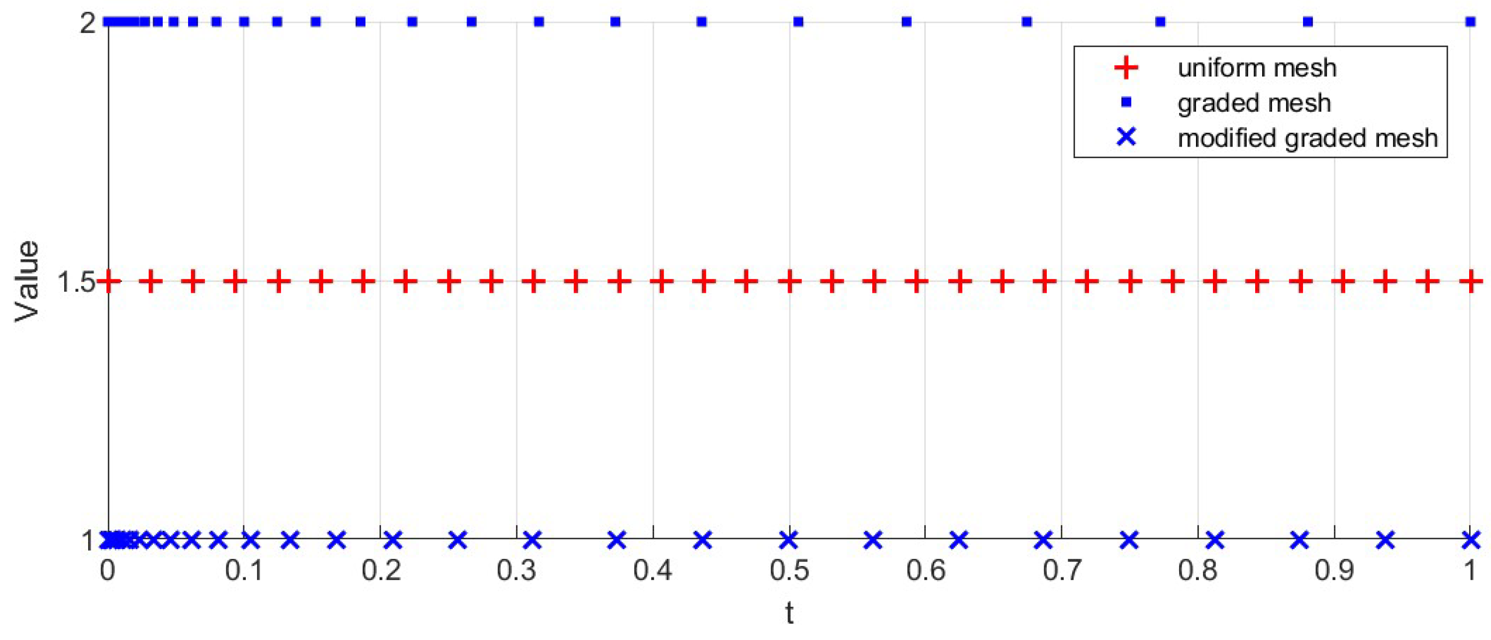
Let N be a positive integer. Let $0=t_0<t_1<\cdots <t_N=T$ be the partition of $[0,T]$. For the graded mesh, we choose $t_k=T{\left({\displaystyle \frac{k}{N}}\right)}^r$, $k=0,1,2,\dots ,N$ with $r\ge 1$. When $r=1$, this mesh is the uniform mesh. For the modified mesh, we have $t_k={\left({\displaystyle \frac{\alpha Pk}{2KN}}\right)}^{{\displaystyle \frac{2}{\alpha }}}$ for $k=0,1,\dots J-1$ and $t_k=\left(1-{\displaystyle \frac{2}{\alpha }}\right)\overline{\sigma }+{\displaystyle \frac{Pk}{TN}}$ for $k=J,J+1,\dots ,N$.

In Figure 1, we choose $N=2048$ and $T=1$ and plot the graded mesh with $r=4$ and uniform mesh with $r=1$ and the modified mesh with $K=0.44,r=4$, and $t_J=0.335596$ with $J=1369$. The modified graded mesh is uneven from $t_0$ to $t_J$, and uniform from $t_J$ to $t_N$.

Figure 1. Three kinds of temporal mesh partitions.

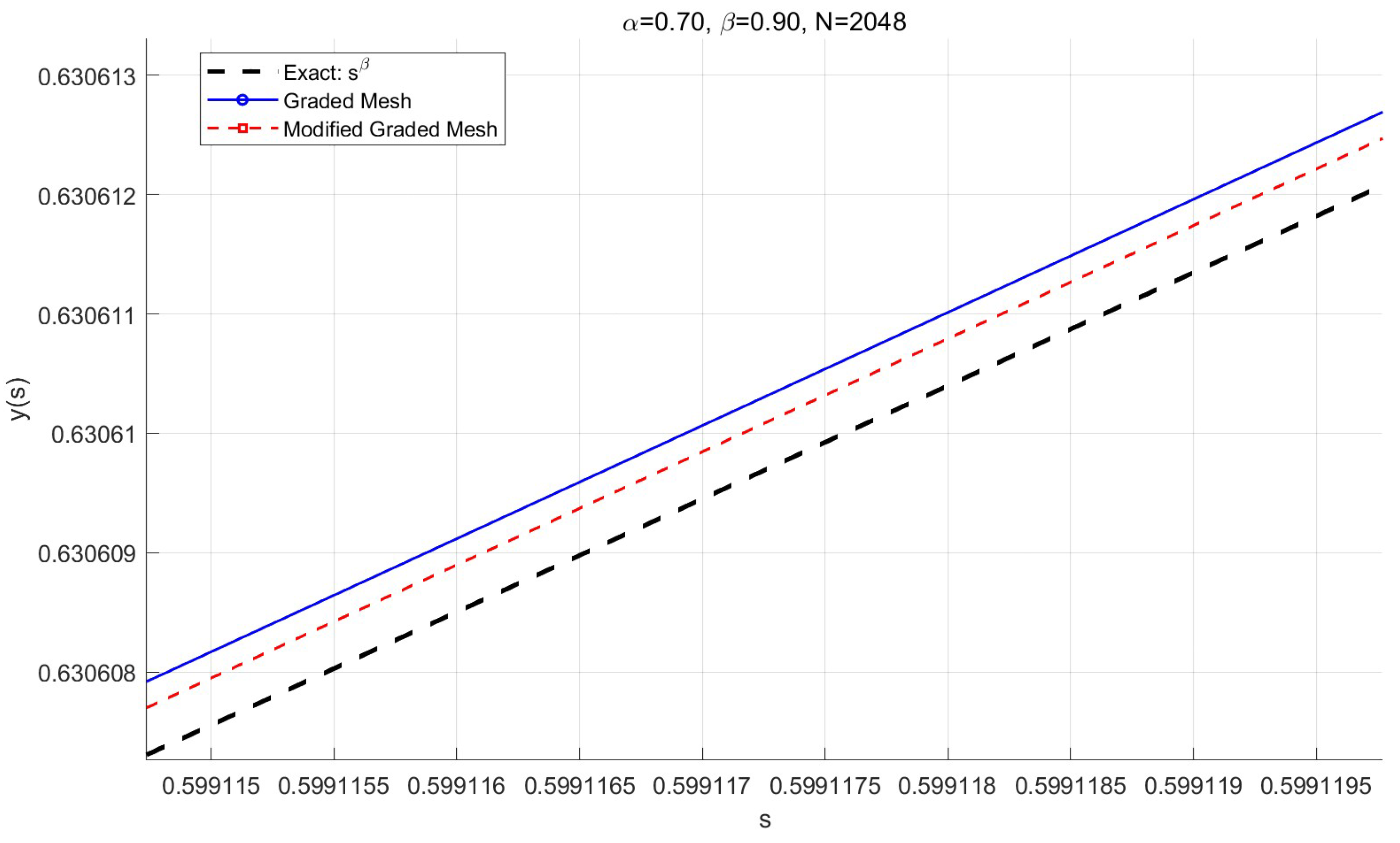
Example 1.

Consider the following fractional differential equation,

$${}_0{}^{C}D_t^{\alpha }u\left(s\right)={\displaystyle \frac{\Gamma (1+\beta )}{\Gamma (1+\beta -\alpha )}}{s}^{\beta -\alpha }+s^{2\beta }-u{\left(s\right)}^2,t\in (0,T],$$

(41)

subject to the initial condition

$$u\left(0\right)=u_0,$$

(42)

where $0<\alpha <1$, $0<\beta <1$, and $\alpha <\beta$, $u_0=0$, and the exact solution is $u\left(t\right)=s^{\beta }$. Here, ${}_0{}^{C}D_t^{\alpha }u\left(s\right)={\displaystyle \frac{\Gamma (1+\beta )}{\Gamma (1+\beta -\alpha )}}{s}^{\beta -\alpha }$, which implies that the regularity of ${}_0{}^{C}D_t^{\alpha }u\left(t\right)$ behaves as $s^{\beta -\alpha }$, which satisfies Assumption 1.

Assume that $u\left(t_k\right)$ and $u_k$, $k=0,1,2,\dots ,N$ are the solutions of (3) and (6), respectively. By Theorem 1 with $\sigma =\beta -\alpha$, we have the following error estimate (note that $t_{n+1}=t_N>t_J$):

$$e_N:=\underset{0\le k\le n+1}{max}|u\left(t_k\right)-u_k|\le C{N}^{-(\alpha +\sigma )}$$

(43)

When $\alpha =0.7$, $\beta =0.9$, $T=1$, and $N=2048$, we compare the exact solution and the numerical solutions for the graded mesh $(r=2.8571)$ and the modified graded mesh $(r=2.8571,K=0.6)$. Figure 2 shows the exact solution along with the numerical solutions obtained using the graded mesh and the modified graded mesh. From the figure, it is evident that both methods approximate the exact solution well, but the modified graded mesh achieves a smaller error compared to the graded mesh. In our numerical tests, we see that the errors from the modified graded mesh depend on the value of K.

Figure 2. The exact solution and the numerical solutions.

For the different values of $\alpha \in (0,1)$, we select the appropriate values of r and set $N=64\times 2^{l-1}$, where $l=1,2,3,4,5,6.$ Then, we compute the maximum nodal error $e_N^{\infty }$ (as previously defined) for various N and determine the experimental order of convergence (EOC) using the following formula:

$${log}_2\left({\displaystyle \frac{e_N^{\infty }}{e_{2N}^{\infty }}}\right).$$

In Table 1, Table 2 and Table 3, we set $\beta =0.9$ and present the experimental order of convergence (EOC) alongside the maximum nodal errors for different values of N. The numerical results indicate that the error of the modified mesh is smaller than that of the graded mesh.

Table 1. Maximum errors at the grid points and convergence rates for Example 1 with parameters $\alpha =0.3$, $\beta =0.9$, $r=6.6667$, $K=0.3$ at $T=t_N=1$.

N	64	128	256	512	1024	2048
G-mesh	$5.2892\times {10}^{-2}$	$1.7169\times {10}^{-2}$	$5.3465\times {10}^{-3}$	$1.7297\times {10}^{-3}$	$5.8865\times {10}^{-4}$	$2.0884\times {10}^{-4}$
	1.6232	1.6832	1.6281	1.5550	1.4950	−
MG-mesh	$1.1599\times {10}^{-2}$	$3.5888\times {10}^{-3}$	$1.1848\times {10}^{-3}$	$4.1230\times {10}^{-4}$	$1.4904\times {10}^{-4}$	$5.5437\times {10}^{-5}$
	1.6924	1.5989	1.5229	1.4680	1.4267	−

Table 2. Maximum errors at the grid points and convergence rates for Example 1 with parameters $\alpha =0.5$, $\beta =0.9$, $r=4$, $K=0.3$, and $T=t_N=1$.

N	64	128	256	512	1024	2048
G-mesh	$4.1827\times {10}^{-3}$	$1.2606\times {10}^{-3}$	$3.9725\times {10}^{-4}$	$1.2959\times {10}^{-4}$	$4.3325\times {10}^{-5}$	$1.4732\times {10}^{-5}$
	1.7303	1.6660	1.6160	1.5807	1.5563	−
MG-mesh	$1.1558\times {10}^{-3}$	$3.6932\times {10}^{-4}$	$1.2194\times {10}^{-4}$	$4.1150\times {10}^{-5}$	$1.4089\times {10}^{-5}$	$4.8689\times {10}^{-6}$
	1.6460	1.5986	1.5673	1.5464	1.5329	−

Table 3. Maximum errors at the grid points and convergence rates for Example 1 with parameters $\alpha =0.7$, $\beta =0.9$, $r=2.8571$, $K=0.5$, and $T=t_N=1$.

N	64	128	256	512	1024	2048
G-mesh	$5.1630\times {10}^{-4}$	$1.4911\times {10}^{-4}$	$4.4181\times {10}^{-5}$	$1.3300\times {10}^{-5}$	$4.0415\times {10}^{-6}$	$1.2353\times {10}^{-6}$
	1.7918	1.7549	1.7320	1.7184	1.7100	−
MG-mesh	$2.4983\times {10}^{-4}$	$7.3910\times {10}^{-5}$	$2.2275\times {10}^{-5}$	$6.7840\times {10}^{-6}$	$2.0783\times {10}^{-6}$	$6.3721\times {10}^{-7}$
	1.7571	1.7304	1.7152	1.7068	1.7055	−

Example 2.

Consider the following

$$\left\{\begin{array}{cc}{}_0{}^{C}D_t^{\alpha }u\left(t\right)+u\left(t\right)=0,\hfill & t\in (0,T],\hfill \\ u\left(0\right)=u_0,\hfill \end{array}\right.$$

where $0<\alpha <1$ and $u_0=1$. The exact solution $u\left(t\right)=E_{\alpha ,1}(-t^{\alpha })$, where $E_{\alpha ,\gamma }\left(z\right)$ is the Mittag-Leffler function defined by

$$E_{\alpha ,\gamma }\left(z\right)={\displaystyle \sum _{k=0}^{\infty }}{\displaystyle \frac{z^k}{\Gamma (\alpha k+\gamma )}},\alpha ,\gamma >0.$$

Hence,

$${}_0{}^{C}D_t^{\alpha }u\left(t\right)=-1-{\displaystyle \frac{(-t^{\alpha })}{\Gamma (\alpha +1)}}-{\displaystyle \frac{{(-t^{\alpha })}^2}{\Gamma (2\alpha +1)}}-\dots ,$$

which suggests that the regularity of ${}_0{}^{C}D_t^{\alpha }u\left(t\right)$ behaves as $c+c{t}^{\alpha }$, where $0<\alpha <1$.

According to Theorem 1, when $\sigma =\alpha$, the error estimate is given by

$$e_N^{\infty }:=\underset{0\le k\le n+1}{max}|u\left(t_k\right)-u_k|\le C{N}^{-2\alpha }.$$

Table 4, Table 5 and Table 6 summarize the experimental order of convergence (EOC) along with the maximum nodal errors for different values of N. The observed EOC closely aligns with the theoretical prediction: $O\left(N^{-2\alpha }\right)$.

Table 4. Maximum errors at the grid points and convergence rates for Example 2 with parameters $\alpha =0.7$, $T=1$, $r=2.8571$, and $K=0.27$.

N	64	128	256	512	1024	2048
G-mesh	$2.5638\times {10}^{-4}$	$7.7441\times {10}^{-5}$	$2.3647\times {10}^{-5}$	$7.2682\times {10}^{-6}$	$2.2630\times {10}^{-6}$	$1.3785\times {10}^{-6}$
	1.7271	1.7114	1.702	1.6833	0.7152	−
MG-mesh	$9.1514\times {10}^{-5}$	$2.8779\times {10}^{-5}$	$9.0681\times {10}^{-6}$	$2.8540\times {10}^{-6}$	$9.0091\times {10}^{-7}$	$3.3928\times {10}^{-7}$
	1.6690	1.6661	1.6678	1.6635	1.4089	−

Table 5. Maximum errors at the grid points and convergence rates for Example 2 with parameters $\alpha =0.8$, $T=1$, $r=2.8571$, and $K=0.1$.

N	64	128	256	512	1024	2048
G-mesh	$1.5459\times {10}^{-4}$	$4.4222\times {10}^{-5}$	$1.2740\times {10}^{-5}$	$3.6820\times {10}^{-6}$	$1.0676\times {10}^{-6}$	$3.2429\times {10}^{-7}$
	1.8056	1.7954	1.7908	1.7861	1.7190	−
MG-mesh	$3.7816\times {10}^{-5}$	$1.1363\times {10}^{-5}$	$3.4120\times {10}^{-6}$	$1.0207\times {10}^{-6}$	$3.0404\times {10}^{-7}$	$9.0227\times {10}^{-8}$
	1.7346	1.7357	1.7411	1.7472	1.7526	−

Table 6. Maximum errors at the grid points and convergence rates for Example 2 with parameters $\alpha =0.9$, $T=1$, $r=2.2222$, and $K=0.58$.

N	64	128	256	512	1024	2048
G-mesh	$9.0168\times {10}^{-5}$	$2.4194\times {10}^{-5}$	$6.5229\times {10}^{-6}$	$1.7627\times {10}^{-6}$	$4.7700\times {10}^{-7}$	$1.3092\times {10}^{-7}$
	1.8980	1.8910	1.8877	1.8857	1.8653	−
MG-mesh	$4.5476\times {10}^{-5}$	$1.2291\times {10}^{-5}$	$3.3370\times {10}^{-6}$	$9.0745\times {10}^{-7}$	$2.4760\times {10}^{-7}$	$7.0494\times {10}^{-8}$
	1.8875	1.8810	1.8787	1.8738	1.8125	−

Through the analysis and numerical experiments, it is clear that the modified graded mesh achieves smaller errors compared to the graded mesh. The traditional graded mesh, with its non-uniform step size, is effective at addressing the weak singularity near the initial time $t=0$. However, as the time nodes $t_k$ move further away from the initial point, the sparsity of the mesh can lead to significant errors. In contrast, the modified graded mesh adopts the graded mesh near $t=0$ to better handle the singularity and transitions to a uniform mesh in later regions, effectively reducing the overall error.

6. Conclusions

In this paper, a modified graded mesh Adams-type predictor–corrector method is proposed for solving fractional differential equations. The traditional graded mesh works well near the initial time $t=0$ because of its non-uniform step sizes, which handle the weak singularity effectively. However, as the time nodes $t_k$ move away from the initial point, the mesh becomes sparse, leading to larger errors. On the other hand, the modified graded mesh uses a graded mesh near $t=0$ to better handle the singularity and switches to a uniform mesh in areas farther from the initial point, significantly reducing the overall error. Numerical experiments further confirm that the modified graded mesh method outperforms the traditional graded mesh in terms of accuracy. This makes the improved Adams-type predictor–corrector method an efficient tool for solving fractional differential equations.

In recent years, some new fractional definitions have been developed, providing new perspectives and tools for the numerical solution of fractional differential equations. Future research directions include extending this method to Caputo–Hadamard fractional derivatives and other fractional definitions (see [27]). We plan to explore numerical methods under these new definitions in future work to further enhance the applicability and accuracy of the proposed approach.