Linear Model and Gradient Feature Elimination Algorithm Based on Seasonal Decomposition for Time Series Forecasting

Abstract

In the wave of digital transformation and Industry 4.0, accurate time series forecasting has become critical across industries such as manufacturing, energy, and finance. However, while deep learning models offer high predictive accuracy, their lack of interpretability often undermines decision-makers’ trust. This study proposes a linear time series model architecture based on seasonal decomposition. The model effectively captures trends and seasonality using an additive decomposition, chosen based on initial data visualization, indicating stable seasonal variations. An augmented feature generator is introduced to enhance predictive performance by generating features such as differences, rolling statistics, and moving averages. Furthermore, we propose a gradient-based feature importance method to improve interpretability and implement a gradient feature elimination algorithm to reduce noise and enhance model accuracy. The approach is validated on multiple datasets, including order demand, energy load, and solar radiation, demonstrating its applicability to diverse time series forecasting tasks.

1. Introduction

With the advent of the Industry 4.0 era, industries such as manufacturing, energy, and finance are undergoing unprecedented digital transformation. This transformation advances automation and signifies a shift toward data-driven intelligent production and decision-making. Accurate time series forecasting is vital to address challenges such as production efficiency, inventory management, energy consumption planning, and financial market prediction. Errors in demand forecasting can lead to serious consequences, including inventory shortages, excess stock, increased costs, or missed business opportunities. Recent developments in machine learning and deep learning models, such as Recurrent Neural Networks (RNNs) [1], Long Short-Term Memory (LSTM) [2], Gated Recurrent Unit (GRU) [3], and Transformer models [4], have significantly improved forecasting accuracy. These models capture nonlinear patterns and long-term dependencies in time series data. However, they often function as black-box models, limiting their interpretability and reducing business decision-makers’ confidence in their results. Understanding the contribution of different features is essential for enhancing trust and optimizing the model.

Interpretability has become a crucial research topic in machine learning. Methods such as Shapley Additive Explanations (SHAPs) [5], Local Interpretable Model-agnostic Explanations (LIMEs) [6], and TimeSHAP [7] provide insights into feature importance for individual predictions. However, these methods are primarily designed for static datasets or classification tasks, and their effectiveness is limited when applied to time series regression models. Furthermore, traditional feature selection methods, such as Recursive Feature Elimination (RFE) [8], are commonly used in static machine learning tasks but are not specifically tailored for time series forecasting, which involves temporal dependencies and dynamic patterns.

To address these challenges, this research proposes a linear time series forecasting model architecture based on seasonal decomposition. Using an additive model, the approach decomposes the time series into trend, seasonality, and residual components. This choice is based on initial data analysis, which revealed that seasonal variations were relatively stable across datasets. Thus, an additive decomposition was deemed appropriate for our data. A multiplicative decomposition would have been more suitable if the seasonal fluctuations had grown or shrunk in proportion to the series level. We further introduce an augmented feature generator to enrich the feature set with differences, rolling statistics, and moving averages to improve predictive performance. Finally, we develop a gradient-based feature importance method and a gradient feature elimination algorithm to provide interpretability and optimize feature selection for time-series-forecasting models.

The proposed method is validated using three datasets: an order demand dataset from a manufacturing company, an energy load dataset, and a solar radiation dataset. Results demonstrate that the proposed approach improves prediction accuracy while enhancing model interpretability, showing its applicability across various domains.

The remainder of this paper is organized as follows—Section 2 reviews related work. Section 3 introduces our approach. Section 4 describes experiments and results. Section 5 concludes the paper.

2. Related Work

2.1. Classical Time-Series-Forecasting Models

Classical statistical models, such as Autoregressive Integrated Moving Average (ARIMA) [9], Kalman Filter (KF) [10], and Exponential Smoothing (ES) [11], have long been regarded as foundational approaches for time series forecasting. ARIMA models rely on differencing, autoregression, and moving averages to handle trends and stochastic behaviors, following the well-known Box–Jenkins methodology. KF methods, on the other hand, recursively compute estimates of a system’s state by minimizing the mean of the squared error, making them effective in systems with continuous updates and noise. ES leverages weighted averages of past observations, placing more emphasis on recent data to capture short-term trends. While these classical models are relatively easy to interpret and effective for stationary or near-stationary time series, they often struggle in scenarios with complex seasonality, nonlinear relationships, or long-range dependencies. Furthermore, they typically assume a fixed functional form and can be sensitive to hyperparameter settings (e.g., ARIMA orders) that may not generalize well across diverse datasets.

2.2. Deep Learning-Based Forecasting Models

In the past decade, deep learning architectures have significantly advanced the capabilities of time series forecasting. Recurrent Neural Networks (RNNs) [1], including Long Short-Term Memory (LSTM) [2] and Gated Recurrent Unit (GRU) [3], were introduced to address the vanishing gradient and long-dependency issues inherent in vanilla RNNs. These models excel at capturing temporal patterns by incorporating gating mechanisms, thus improving gradient flow over long sequences. However, as sequences become incredibly long, training can become computationally expensive, and some information may still be lost due to its recurrent nature.

Transformer-based models [4] have revolutionized sequence learning with the self-attention mechanism, allowing for parallel processing of input elements. Informer [12], Autoformer [13], and FEDformer [14] extend the Transformer architecture for more efficient long-sequence processing by employing novel attention mechanisms or decomposition strategies. Mamba [15] introduces a selective state space approach, updating hidden states efficiently while preserving crucial information from distant time steps. Despite their high performance, these models can sometimes be overkill for datasets lacking complex dependencies, and their interpretability remains challenging without additional techniques.

2.3. Linear Models for Long-Term Forecasting

Contrary to the growing complexity of deep learning models, recent studies have revisited linear approaches for long-term time series forecasting. Zeng et al. [16] proposed LTSF-Linear, demonstrating that simple linear models can match or even surpass Transformer-based methods on specific datasets, especially for extended forecasting horizons. The simplicity of linear models offers faster training, lower memory usage, and improved interpretability. Their limitations lie in the assumption of linear relationships, which might not hold for highly nonlinear series. Nonetheless, when combined with suitable data preprocessing techniques—such as trend/seasonality extraction—they can serve as a robust baseline or a preferred choice, especially in resource-constrained or high-interpretability scenarios.

LTSF-Linear regresses historical time series with a one-layer linear model that captures short-term and long-term temporal relationships and predicts future time series. LTSF-Linear can be mathematically expressed as follows:

$${\widehat{X}}_i=W{X}_i$$

(1)

where $W\in {\mathbb{R}}^{T\times L}$ is a linear layer along the temporal axis, with different variables sharing the same weights and not modeling any spatial correlations. ${\widehat{X}}_i$ and $X_i$ are the predicted and input values for each $i$-th variable, respectively.

The entire process can be represented as follows:

$${\widehat{X}}_i=H_s+H_t$$

(2)

where $H_s=W_s{X}_s\in {\mathbb{R}}^{T\times C}$ and $H_t=W_t{X}_t\in {\mathbb{R}}^{T\times C}$ are the decomposed trend and seasonality sequences. $W_s\in {\mathbb{R}}^{T\times L}$ and $W_t\in {\mathbb{R}}^{T\times L}$ are two linear layers, as shown in Figure 1.

LTSF-Linear includes two variants with different data-preprocessing methods, DLinear and NLinear, to handle time series from various domains. DLinear combines the sequence decomposition method and linear layers used in Autoformer [13] and FEDformer [14]. It first uses the moving average method to decompose the raw input data, extracting the trend sequence and treating the difference between the original sequence and the trend sequence as the seasonal sequence. Then, it applies two single-layer linear layers to each sequence and sums the results to obtain the final prediction. On the other hand, NLinear is suitable for cases where the dataset exhibits distributional shifts. The NLinear model subtracts the last value of the sequence from the input. After passing through the linear layer, the previously subtracted part is added back before making the final prediction. The subtraction and addition in NLinear can be seen as normalizing the input sequence.

2.4. Feature Selection and Importance Estimation

Feature selection and importance estimation are pivotal in improving model accuracy and facilitating interpretability. Recursive Feature Elimination (RFE) [8] is a widely adopted technique that repeatedly removes the least essential features based on model performance. While RFE has proven effective for static datasets, it often disregards temporal order and dependencies in time series. Interpretability methods such as SHAP [5], LIME [6], and TimeSHAP [7] help explain model decisions by estimating the contribution of input features. However, these approaches target classification tasks or static tabular data, limiting their direct applicability to time series regression. In a time series context, features may represent lagged values, moving averages, or seasonal transformations, necessitating specialized feature selection algorithms that account for temporal continuity and the changing relevance of features over time.

2.5. Seasonal Decomposition and Hybrid Models

Seasonal decomposition techniques, such as classical decomposition and STL (Seasonal-Trend decomposition using Loess) [17], have been extensively used to separate a time series into trend, seasonal, and residual components. By isolating these components, researchers and practitioners can model each part with a tailored approach. For instance, Zhang [18] combined a decomposed linear model with a neural network, leveraging the strengths of both methods. Wavelet decomposition and other advanced transforms have also been explored to capture multi-scale behaviors in complex series. These hybrid or ensemble methods underscore the potential of decomposition to simplify data patterns, making downstream modeling more accurate and interpretable. Nevertheless, integrating decomposition with automated feature selection—while preserving interpretability—remains an open challenge.

In summary, the literature reveals a spectrum of approaches for time series forecasting, ranging from classical statistical methods and deep neural networks to linear models and decomposition-based hybrids. However, few works directly integrate decomposition with a gradient-based feature importance framework to simultaneously address nonlinearities, long-range dependencies, and feature interpretability. Our research aims to fill this gap by proposing a linear model architecture with seasonal decomposition, augmented feature generation, and a gradient feature elimination algorithm.

3. Approach

In our research, we propose a linear time series model architecture based on seasonal decomposition, combined with an augmented feature generator to produce augmented features, further improving the model’s accuracy in predicting order demand for the coming weeks and addressing inventory issues. Additionally, we introduce a gradient-based feature importance method to provide interpretability to complex time series models. Using this method, we also implement a gradient feature elimination algorithm to reduce noise and overfitting, further optimizing model accuracy.

Finally, to comprehensively evaluate the effectiveness of our proposed method, we tested it using private datasets and two different open-source datasets: a machine energy consumption dataset and a solar radiation energy dataset. The selection of these datasets demonstrates the generalizability and performance of our method across different types of time-series-forecasting problems.

3.1. Architecture

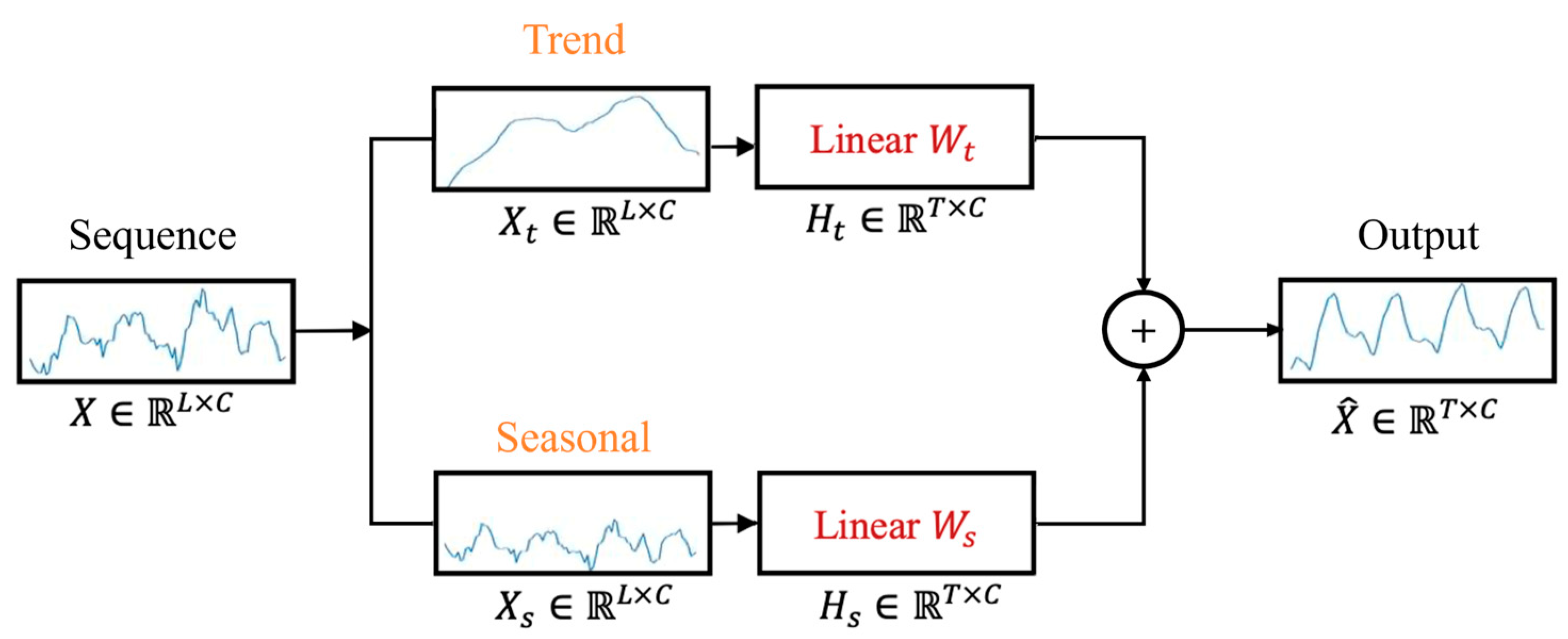
This study proposes a time-series-forecasting framework based on a seasonal decomposition linear model for time series prediction tasks. This framework combines an augmented features generator and a gradient feature importance method to optimize model performance and interpretability. First, we decompose the target data using the seasonal decompose function mentioned in Section 3.4, dividing the time series into trend, seasonality, and residual components. This allows the model to make predictions based on the decomposed trend and seasonal time series data, thereby improving prediction accuracy.

Next, we use the Augmented Features Generator proposed in Section 3.5 for the target data to generate augmented features. These features include differences, rolling statistics, exponential moving averages, rates of change, and Fourier transforms to comprehensively capture the time series characteristics.

To fully utilize the decomposed time series, augmented features, and support data, we preprocess all data using the data-preprocessing methods mentioned in Section 3.3, converting it into a format suitable for training time series models. Then, we use the DLinear model discussed in Section 2. We train two DLinear models, one focusing on the trend and the other on seasonality, allowing the models to specialize in individually predicting trend and seasonal components.

After training the models, we use the gradient feature importance method proposed in Section 3.6 to generate the current gradient feature importance results, providing interpretability for the complex time series model. We employ the gradient feature elimination algorithm described in Section 3.7 to improve model prediction accuracy further. This algorithm iteratively removes features with the lowest gradient importance, reducing model complexity and preventing overfitting, thereby enhancing prediction accuracy.

Finally, we combine the trend, seasonality, and residual component predictions to obtain the final prediction results. The overall architecture is shown in Figure 2.

3.2. Time Series Data Definition

Time series data refers to data collected, recorded, or measured at consecutive time points and is characterized by data points that vary over time. This paper uses multidimensional data, including target sequences and support sequential data, to infer predictions for single or multiple time points. Here is our data definition:

• Target data: This is the primary series for which we wish to make predictions, using past time points to forecast future values. The target data $T$ is a vector comprising values representing the target variable over a series of time points, denoted by $t_i$, where $n$ is the number of time points in the data, and mathematically represented as $T={\left[t_1,t_2,\dots ,t_n\right]}^T$, with $T^T$ indicating the transpose of the vector.
• Support data: These are support data sequences related to the forecasting target sequence. These sequences are typically used as additional information to aid in predictions. The $j$-th support data $O_j$ is represented as a vector containing values representing the $j$-th variable over a series of time points, denoted by $o_{ji}$, where $n$ is the number of time points in the data, and mathematically represented as $O_j={\left[o_{j1},o_{j2},\dots ,o_{jn}\right]}^T$, with $O_j^T$ indicating the transpose of the vector.
• Multidimensional data X: This integrates the target data $T$ and support data $O_1,O_2,\dots ,O_m$, where each row represents a time point, consisting of the values of the target variable in the first column, and the values of support variables from $O_1,O_2,\dots ,O_m$ in subsequent columns. $X$ can be represented as a matrix:

  $$X=\left[\begin{array}{ccccc}{t}_1& o_{11}& o_{21}& \cdots & o_{m1}\\ t_2& o_{12}& o_{22}& \cdots & o_{m2}\\ ⋮& ⋮& ⋮& \ddots & ⋮\\ t_n& o_{1n}& o_{2n}& \cdots & o_{mn}\end{array}\right]$$

  (3)

This multidimensional data framework facilitates in-depth analysis of time series, enhancing the accuracy and reliability of forecasting models by comprehensively considering both the target data and its related support data.

3.3. Data Processing

(1)

Normalization

During the training of machine learning models, significant discrepancies in the numerical range of raw data can adversely affect the learning efficacy of the models, especially when using gradient descent-based algorithms where the objective function may not operate properly. To facilitate better learning by the model, we employ min–max scaling to preprocess the data, adjusting all feature values in the raw data to a range of the following $\left[\mathrm{0,1}\right]$:

$$x_{norm}={\displaystyle \frac{x-\min \left(x\right)}{max\left(x\right)-min\left(x\right)}}$$

(4)

where $x_{norm}$ represents the normalized data, $x$ represents the original data, and $min\left(x\right)$ and $max\left(x\right)$ are the minimum and maximum values of the original data, respectively.

(2)

Serialize Data

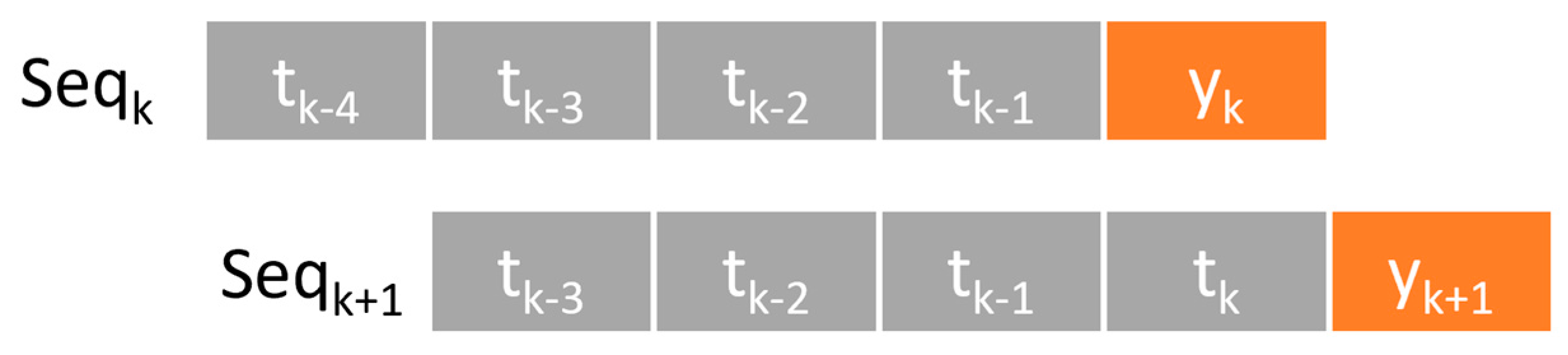
In the training process of time series models, it is essential to transform the data into a suitable format. The window-sliding method accomplishes this transformation. The principle of window sliding involves moving a fixed-size window over the time series data, organizing the data within each window into a sequence, and using the value of the next time step at the end of each window as the prediction target, as shown in Figure 3. For cases with only the target sequence, we represent the sequence as a vector of time series $\{t_1,t_2,\dots ,t_n,y_t\}$, where $t_i$ represents the values from previous time points within the window, $n$ represents the number of time points, indicating the number of prime time points included in each sequence, and $y_t$ is the target value to predict. For multidimensional scenarios, the sequence is represented as $\{t_1,o_1^1,o_1^2,\dots ,o_1^m,\dots ,t_n,o_n^1,o_n^2,\dots ,o_n^m,y_t\}$, where $t_i$ indicates the values from the target sequence at the $i$-th time point within the window, $o_i^j$ are values from support sequences $O_j$, with $o_i^j$ representing the value of the $j$-th support sequences at the $i$-th time point within the window, $m$ being the number of support sequences in the multidimensional time series, $n$ representing the number of time points, and $y_t$ being the target value to predict.

For each sequence set, including target and multidimensional sequences, we can represent it as follows:

• Target sequence:

$$Se{q}_k=\{t_{k-W},t_{k-W+1},\dots ,t_{k-1},y_k\}$$

(5)

where $t_i$ indicates data points in the time series, $y_k$ is the target prediction value, $k$ is the current time point index, and $W$ is the window size.

• Multidimensional sequence:

$$Se{q}_k=\{t_{k-W},o_{k-W}^1,\dots ,o_{k-W}^m,\dots ,t_{k-1},o_{k-1}^1,\dots ,o_{k-1}^m,y_k\}$$

(6)

where $o_i^j$ represents the value of the $j$-th support sequence at time point $i$, and $m$ is the total number of support sequences.

(3)

De-Normalization

After the model completes its predictions, we must transform the predicted results back to the original data’s numerical range to compare the expected sequence and measure the model’s performance. This process is called de-normalization, and its formula is as follows:

$$x_{original}=x_{norm}\times \left(max\left(x\right)-min\left(x\right)\right)+min\left(x\right)$$

(7)

where $x_{norm}$ is the normalized prediction result, $x_{original}$ is the de-normalized prediction result, and $min\left(x\right)$ and $max\left(x\right)$ are the minimum and maximum values of the original data $x_{original}$, respectively.

3.4. Seasonal Decomposition

In time series analysis, seasonal decomposition is a common technique to identify and decompose a sequence into trend, seasonality, and residual components. In this study, we employ the seasonal decompose function from Python’s stats models library to implement seasonal decomposition. This function uses moving average techniques to extract the trend from the time series and calculate the seasonality and residuals accordingly, enhancing subsequent model predictions’ accuracy.

Seasonal decomposition breaks the time series into three subseries:

• Trend: Represents the long-term changes in the time series. It shows whether the overall trend of the data over time is upward, downward, or stable. The trend is obtained using moving averages as a filter.
• Seasonality: Captures the seasonal patterns within the series, i.e., repetitive behaviors occurring at fixed time intervals. The seasonality is the average of the detrended series for each period.
• Residual: Comprises parts of the data that cannot be explained by the trend and seasonality, also known as random fluctuations or noise. Residuals contain other influencing factors not captured by the model, such as sporadic events or random fluctuations. Residuals are calculated by removing the trend and seasonality from the original series.

We expect the model to exhibit improved predictive accuracy when dealing with decomposed trend and seasonal time series data through this decomposition technique.

The seasonal decompose function supports two decomposition models: additive and multiplicative.

(1)

Additive Model

The additive model assumes that the time series is a linear combination of trend, seasonality, and residuals. It can be represented as follows:

$$Y\left[t\right]=T\left[t\right]+S\left[t\right]+e\left[t\right]$$

(8)

where $Y\left[t\right]$ is the original time series value at time $t$, $T\left[t\right]$ is the trend component, $S\left[t\right]$ is the seasonal component, and $e\left[t\right]$ is the residual.

(2)

Multiplicative Model

The multiplicative model assumes that the time series is a product of the trend, seasonality, and residuals. It is typically used when significant seasonal variations are related to the trend. It can be expressed as follows:

$$Y\left[t\right]=T\left[t\right]\times S\left[t\right]\times e\left[t\right]$$

(9)

where each term has the same meaning as the additive model.

Additive vs. Multiplicative Seasonality—When to Use Which: The key distinction between these models lies in whether seasonal fluctuations remain constant or vary with the overall level of the series. In an additive decomposition, seasonal effects are roughly constant in amplitude regardless of the trend level, making it suitable when seasonal patterns do not scale with the series. In contrast, a multiplicative decomposition is appropriate when seasonal effects scale proportionally with the trend (for example, when higher sales volumes come with proportionally more significant seasonal increases). This difference is also reflected in how seasonal indices are calculated. For an additive model, seasonal index (e.g., monthly or weekly seasonal effects) are typically computed by taking the arithmetic mean of the detrended values for each season, and they are often normalized to sum to zero over a complete cycle (ensuring no net seasonal bias is added). For a multiplicative model, seasonal indices are derived as ratios of the original values to the trend (or deseasonalized values), and these factors are usually normalized so that their geometric mean equals one over a cycle (ensuring no overall scale change is introduced). In practice, if the seasonal pattern’s amplitude increases or decreases with the series level, a multiplicative approach (sometimes after transforming the data logarithmically) would capture the dynamics better; otherwise, the additive approach is preferred. In our case, initial exploration of the datasets indicated that an additive seasonal effect was adequate, as seasonal fluctuations were relatively stable and did not exhibit strong dependence on the trend component.

The framework isolates the trend and seasonal components by decomposing each time series using the appropriate model (additive in this study). We expect the model to exhibit improved predictive accuracy when dealing with these separated components since it can independently focus on learning the trend and seasonality patterns rather than the conflated raw series. Any unexplained variation remains in the residual component, which contains factors not captured by the model (such as sporadic events or random noise). These residuals are calculated by removing the estimated trend and seasonal components from the original series.

3.5. Augmented Features Generator

In this section, we introduce an augmented features generator to create additional features from the original target sequence, aiming to improve the predictive accuracy of our time series model. These features include first- and second-order differences, rolling statistics, exponential moving averages, rates of change, and Fourier transform features, among others, to capture the time series characteristics comprehensively.

(1)

First and Second-Order Difference Features

Calculating a time series’ first- and second-order differences is a common technique to stabilize a non-stationary series, making patterns more straightforward to model. The first-order difference (the difference between adjacent time points) often removes a constant trend component and highlights short-term changes. The second-order difference (the difference in the first-order differences) helps capture the acceleration or deceleration in the rate of change in the data, making it particularly useful for detecting more complex or nonlinear trends in the data. By applying these differencing operations, we mitigate underlying trend effects or seasonality to some extent and stabilize the series, leading to more reliable predictions by the model on the transformed data.

(2)

Rolling Statistical Features

Rolling statistical features, calculated using a moving window, capture local properties of the sequence and extract time-related information. These features compute statistics (such as maximum, minimum, mean, standard deviation, median, and percentiles) over a fixed-size window that slides through time. At each time step, the window yields a statistic summarizing the recent history, thereby providing the model with contextual information about recent values. Rolling features can highlight local trends and variability that single-point observations cannot.

(3)

Exponential Moving Average (EMA)

The exponential moving average is a smoothing technique that reduces short-term noise in the data. It assigns exponentially decaying weights to past observations, giving more weight to recent data points. This helps capture recent trends or shifts faster than a simple moving average while smoothing out irregular fluctuations.

(4)

Rate of Change

The rate of change measures the relative change between consecutive data points, often expressed as a percentage. This feature indicates the series’ momentum—whether values increase or decrease and how rapidly. By including the rate of change, the model can capture sudden jumps or drops and steady growth/decline patterns in the time series.

(5)

Fourier Transform Features

The Fourier transform decomposes a time series into a spectrum of frequencies. We can identify dominant cyclic patterns by converting the time-domain data into the frequency domain. In our feature set, we include characteristics derived from the Fourier transform (such as the prominent frequency components’ amplitudes and phases or summary statistics like the mean of real/imaginary parts) to help the model recognize seasonality or periodic behavior that might not be immediately obvious in the time domain.

(6)

Lag Features

We also include lag features, simply past values of the target time series used as additional inputs for forecasting. By feeding the model recent historical values (e.g., the value one-time step ago, two-time steps ago, etc.), we enable it to capture temporal dependencies directly. Lag features are a straightforward yet powerful way to incorporate autoregressive information into the model.

3.6. Gradient Feature Importance

In our research, we propose a gradient-based feature importance method as an innovative explainability framework to address the challenge of interpretability in time-series-forecasting models. Traditional model interpretation methods, such as SHAP [5], LIME [6], and Anchors [19], while influential in many domains, encounter limitations when interpreting time series models. These methods typically ignore the sequential nature of data or are designed for classification contexts. TimeSHAP [7] provides some interpretability for RNN predictions by perturbing sequences, but it has not been adapted for regression tasks in time series.

Instead, our gradient feature importance approach leverages the model’s gradients concerning input features to quantify each feature’s contribution to the prediction. This method directly applies to our linear model and augmented features framework, offering insight into how each feature (including those generated by the augmented features generator) influences the forecast.

Using gradients for importance has the advantage of being model-specific and sequence-aware: it considers how slight changes in a feature at a given time step would affect the prediction, thereby capturing the temporal context. We compute the gradient of the model’s output concerning each input feature dimension; a larger magnitude indicates that changes in that feature would significantly impact the prediction, hence higher importance. By averaging or otherwise aggregating these gradient-based importance scores over the evaluation period, we obtain an importance ranking of features for the model’s forecasting task. This gradient feature importance forms the basis for the subsequent feature elimination strategy.

The gradient feature importance results are illustrated in Figure 4. As shown, ‘Quantity_in_stock’ emerges as the most significant feature, followed by ‘change_rate’, ‘rolling_max’, and others. The least important feature is ‘Inbound’. The pseudocode for the algorithm is presented in Algorithm 1.

Algorithm 1 Gradient Feature Importance Algorithm

Input: Trained model M, Training dataset $D\{(x_1,y_1),\dots ,(x_n,y_n)\}$, Feature set $F\{f_1,f_2,\dots ,f_n\}$, Number of features N. Output: Importance score for each feature $f_j$. 1: $I\left(F\right)\leftarrow \{0,0,\dots ,0\}$   ▷ Initialize importance scores 2: for each $(X_i,y_i)$ in D do 3:    ${\widehat{y}}_i=M\left(x_i\right)$ 4:    $\mathcal{L}\leftarrow \mathrm{Loss}({\widehat{y}}_i,y_i)$    ▷ Compute loss 5:    for each feafure fj in F do 6:     $I\left(f_j\right)\leftarrow I\left(f_j\right)+\left|{\displaystyle \frac{\partial \mathcal{L}}{\partial f_j}}\right|$    ▷ Accumulate absolute gradient 7:    end for 8: end for 9: for each feafure fj in F do 10:     $\mathit{I}\left({\mathit{f}}_{\mathit{j}}\right)\mathbf{\leftarrow }{\displaystyle \frac{\mathit{I}\left({\mathit{f}}_{\mathit{j}}\right)}{\mathit{N}}}$    ▷ Calculate the average gradient 11: end for 12: return $I\left(F\right)$    ▷ Return importance scores for all features

3.7. Gradient Feature Elimination

Building on the importance ranking, we implement a gradient feature elimination algorithm to iteratively remove less essential features and observe the impact on model performance. Starting with the complete feature set (including all augmented features), we gradually eliminate the feature with the lowest importance score and retrain or re-evaluate the model. If the model’s accuracy remains acceptable (or improves due to noise reduction), we continue eliminating the next least important feature. This process continues until removing any additional feature causes a significant drop in performance, indicating that all remaining features are crucial. The result is a simplified model with a smaller set of features, often leading to reduced overfitting risk, improved generalization, and more straightforward interpretability since fewer features are involved. We provide the results of this procedure in the Experimental Section to demonstrate how feature elimination based on gradient importance can maintain or even enhance forecasting accuracy while using a more parsimonious input feature set.

The algorithm pseudocode is shown in Algorithm 2.

Algorithm 2 Gradient Feature Elimination Algorithm
Input: Trained model M, Training dataset $D=((x_1,y_1),\dots ,(x_n,y_n))$, Number of Features N, P is patience. Output: Reduced feature set
1: $F\leftarrow \{f_1,f_2,\dots ,f_N\}$	▷ Initialize feature set
2: ${\mathcal{L}}_{\mathcal{b}\mathcal{e}\mathcal{s}\mathcal{t}}\leftarrow \mathrm{\infty }$	▷ Initialize best validation loss
3: $p\leftarrow 0$	▷ Initialize patience counter
4: while $\left|F\right|>0$ do
5:   $I\left(F\right)\leftarrow \mathbf{GradientFeatureImportance}(M,D,F)$
6:   $f_{min}\leftarrow argminI\left(F\right)$	▷ Find feature with lowest importance
7:   $F\leftarrow F\setminus \left\{f_{min}\right\}$	▷ Remove least important feature
8:   Retrain model M using feature set F
9:   Evaluate validation loss ${\mathcal{L}}_{\mathcal{v}\mathcal{a}\mathcal{l}}$	▷ Evaluate model performance
10:  if ${\mathcal{L}}_{\mathcal{v}\mathcal{a}\mathcal{l}}<{\mathcal{L}}_{\mathcal{b}\mathcal{e}\mathcal{s}\mathcal{t}}$ then
11:   ${\mathcal{L}}_{\mathcal{b}\mathcal{e}\mathcal{s}\mathcal{t}}\leftarrow {\mathcal{L}}_{\mathcal{v}\mathcal{a}\mathcal{l}}$	▷ Update best validation loss
12:   $p\leftarrow 0$	▷Reset patience counter
13:  else
14:   $p\leftarrow p+1$	▷Increment patience counter
15:  end if
16:  if $p\ge P$ then
17:   return F	▷Return reduced feature set
18:   end if
19: end while
20: return F	▷Return reduced feature set

3.8. Calculate Inventory Improvement from the Order Dataset

With the advent of Industry 4.0, the manufacturing sector actively pursues intelligent management models, where inventory management is critical. To effectively reduce inventory levels, we rely not only on the internal customer order quantities introduced by ERP systems but also utilize our proposed linear time series model architecture based on seasonal decomposition and augmented features with an augmented features generator to improve forecast accuracy. Further, we integrate the gradient feature importance method and gradient feature elimination algorithm to ensure the interpretability of the forecast results and optimize the model.

Finally, we calculate the improvement in inventory based on the forecast results to verify whether our proposed method can effectively reduce inventory levels and address issues of inventory shortages. Through such methods, we aim to achieve more competent inventory management in manufacturing, thereby reducing costs and better meeting customer demands.

• Updating Weekly Inventory Levels

First, we update the weekly inventory levels based on the quantities of incoming and outgoing goods using the following calculation:

$$Q_{i+1}=Q_i+I_i-O_i$$

(10)

where $Q_{i+1}$ is the inventory level for week $i$ + 1, $Q_i$ is the inventory level for week $i$, $I_i$ is the quantity of goods received during week $i$, and $O_i$ is the quantity of goods dispatched during week $i$.

• Calculating Post-Forecast Inventory Levels

To calculate the post-forecast inventory levels, we subtract the actual order quantity from the forecasted order quantity each week and then add this difference to the initial inventory level. In other words, the new inventory level is the initial inventory level plus the cumulative difference between forecasted and actual order quantities:

$${\widehat{Q}}_{i+1}=Q_{init}+{\sum }_{i=1}^n(P_i-A_i)$$

(11)

where ${\widehat{Q}}_{i+1}$ is the post-forecast inventory level, $Q_{init}$ is the initial inventory level, $P_i$ is the forecasted order quantity for week $i$, $A_i$ is the actual order quantity for week $i$, and $n$ is the total number of weeks.

• Comparing Inventory Level Changes

Finally, we compare the post-forecast inventory level with the original inventory level to assess the improvement in inventory management. If the post-forecast inventory level is higher than the original, it indicates an improvement in inventory management; otherwise, it may indicate a deterioration. To evaluate the effectiveness of inventory management improvements, we calculate the percentage difference between the post-forecast and original inventory levels:

$${\displaystyle \frac{{\widehat{Q}}_{i+1}-Q_i}{Q_i}}\times 100$$

(12)

where ${\widehat{Q}}_{i+1}$ represents the post-forecast inventory level, and $Q_i$ represents the original inventory level for a week $i$.

Through the methods described above, we can calculate the improvement in inventory from the order forecast dataset, thereby guiding manufacturers to adjust their inventory management strategies and reduce inventory costs.

4. Implementation and Experiments

4.1. Datasets and Environment

(1)

Datasets

Datasets: We utilized three datasets to validate our model. The first dataset consists of weekly order data from a collaborating manufacturer’s ERP (Enterprise Resource Planning) system. In addition to customer product orders, we calculated weekly inventory inputs, outputs, transaction quantities, and stock levels as part of this dataset, yielding several features related to inventory movement. The prediction target for this dataset is the customer order quantity. By forecasting this target, we aim to convert the predictions into order recommendations that help reduce the number of weeks with insufficient inventory and optimize overall inventory levels.

The second dataset is a public electric load dataset containing energy load readings for a specific machine collected over time. This dataset spans from November 2016 to November 2019. Features provided include the machine’s energy load and environmental or temporal context features, such as low temperature, high temperature, and time attributes (year, month, day, and hour). In this case, the prediction target is the machine’s energy consumption (Load). These additional features allow the model to account for daily and seasonal temperature effects or time-of-day usage patterns that might influence the energy load.

The third dataset is a public solar radiation dataset consisting of meteorological data from the HI-SEAS weather station, covering four months from September 2016 to December 2016. This dataset includes six features: solar radiation (the target variable to forecast), temperature, humidity, and barometric pressure. The goal is to predict solar radiation energy based on the recent history of these variables, which is relevant for applications like solar panel output forecasting or climate analysis.

Table 1. List of three datasets.

Datasets	Time Range	Features	Train	Validation	Test
Order	2020/03–2023/08	5	162	19	19
Electric load	2016/11–2019/11	7	21,024	2628	2628
Solar radiation	2016/09–2016/12	5	26,148	3269	3269

below summarizes the key details of these three datasets, including the data collection period (Time Range), the number of features, and the train/validation/test split sizes.

(2)

Time-Series Visualization Analysis

Exploratory data analysis of the above datasets provides insight into their trend and seasonal characteristics. In Figure 5, we visualize the time series of each dataset to assess the presence of trends and seasonality and determine the nature of any seasonal effects (additive or multiplicative).

• Order dataset: The weekly order time series (2020/03–2023/08) exhibits a notable upward trend over the three years, indicating increasing order quantities over time. We also observe a repeating pattern that corresponds roughly to annual seasonality—for instance, peaks and troughs occurring at similar times each year—suggesting a seasonal effect. The amplitude of these seasonal fluctuations remains relatively consistent from year to year despite the rising trend (i.e., the seasonal peaks increase roughly in line with the overall growth but not disproportionately so). This indicates an additive seasonal effect: the seasonal component adds a similar absolute amount each year. In other words, the seasonal pattern is stable (the difference between peak and trough orders is about the same each year), and it does not scale with the level of the series. This visual observation supports our additive decomposition model for the order dataset’s seasonality. In Figure 5 are time series plots of the order datasets in Table 1. Each subplot shows the entire dataset time, illustrating trends and seasonal patterns.
• Electric load dataset: The machine energy load series (2016/11–2019/11) shows a strong periodic pattern corresponding to daily and weekly cycles. The visualization shows a regular cyclical fluctuation every 24 h (high loads during certain hours and lower during others) and a repeating weekly pattern (differences between weekdays and weekends, for example). There is no clear long-term upward or downward trend over the three years; the baseline load level appears relatively steady aside from routine fluctuations. The seasonality in this context is the daily cycle (and possibly weekly pattern), and its magnitude does not change significantly over time—peak usage each day remains in a similar range throughout the dataset. This suggests an additive seasonal effect for the electric load data as well. The seasonal component (daily usage pattern) adds and subtracts roughly the same load regardless of the month or year. We do not see the seasonal amplitude growing or shrinking systematically over the years, meaning a multiplicative model is unnecessary here. The consistent daily cycle confirms that additive decomposition is suitable for isolating the recurring patterns in this dataset. In Figure 6 are time series plots of the Electric Load dataset in Table 1. Each subplot shows the entire dataset time, illustrating trends and seasonal patterns.
• Solar radiation dataset: The solar radiation series (2016/09–2016/12) is dominated by a pronounced daily cycle due to the day–night alternation. Each day shows a sharp increase in radiation in the morning, a peak around midday, and a decline to zero at night. Over the four months, there is a slight trend: the peak daily radiation tends to decline as the months progress from September into December, reflecting shorter days and lower solar angles in late autumn. Despite this downward trend in the overall level of radiation, the seasonal pattern (daily cycle) is pretty regular in shape. The daytime peak’s amplitude decreases moderately from September to December, but this can largely be attributed to the trend of changing seasons (moving toward winter) rather than a change like daily fluctuations. Because the baseline at night is zero, a purely multiplicative seasonal model is impractical (multiplicative decomposition would imply zero seasonal factors at night). Instead, we treat the daily cycle as an additive seasonal effect superimposed on a slowly declining trend. The seasonal component contributes roughly the same form each day (with its peak height gradually decreasing in tandem with the trend). An additive model can adequately capture this behavior: the diminishing peak is interpreted as the trend component reducing over time, while the seasonal component remains similar. Thus, we apply an additive decomposition for the solar radiation dataset—the daily seasonality is added to a downward trend over the four months. Figure 7 shows time series plots of the solar radiation datasets in Table 1. Each subplot shows the entire dataset time, illustrating trends and seasonal patterns.

Our visual analysis of all three datasets reveals that each time series contains identifiable trend and seasonal components. Crucially, the seasonal effects appear additive for all cases: seasonal patterns maintain a relatively constant magnitude and do not scale multiplicatively with the overall level of the series. As implemented in our proposed model, these observations justify additive seasonal decomposition across the datasets. If any dataset had shown clear evidence of seasonality with amplitude proportional to its trend (which would indicate a multiplicative effect), we would have adjusted our approach accordingly; however, no such behavior was observed in these three cases.

(3)

Environment

All model training and experiments were conducted on a machine with an NVIDIA RTX A6000 GPU (NVIDIA, Santa Clara, CA, USA).

Table 2. Experiment environment.

Item	Content
OS	Ubuntu 20.04.6 LTS
Python	3.9.18
Cuda	11.6
PyTorch	2.2.0
CPU	AMD Ryzen 9 5950X 16-Core Processor (AMD, Santa Clara, CA, USA)
GPU	NVIDIA RTX A6000 (NVIDIA, Santa Clara, CA, USA)
RAM	64 G

details the software and hardware environment used. The models were implemented in PyTorch 2.2.0 and trained under Ubuntu Linux.

4.2. Training Procedure and Evaluation Metrics

(1)

Seasonal Decomposition and Data Restoration

In our research framework, seasonal decomposition on the target variable is necessary. Seasonal decomposition divides the time series data into trend, seasonal, and residual components. As mentioned in Section 3.4, the sum of these three sub-series equals the original series. We use the trend and seasonal components, combined with support data, to train the models separately. Finally, we need to restore the decomposed data to evaluate prediction accuracy. Therefore, we sum the model-predicted trend, seasonal components, and the residual values obtained through seasonal decomposition to derive the complete prediction results.

(2)

Experimental Setup

Before training the models, we split the datasets into training, validation, and testing sets in an 8:1:1 ratio. The common hyperparameters set for all models are as follows: The number of training epochs is 200, and the batch size is 400, or the highest possible size if the data are insufficient. The time series length is 60, and the mean squared error (MSE) is the loss function. The optimizer is adaptive moment estimation (Adam) with an initial learning rate of 0.001. The learning rate is reduced by 10% if there is no improvement in validation accuracy for nineteen epochs.

(3)

Evaluation Metrics

In this study, we employ multiple metrics to assess our time series prediction models. We chose Mean Square Error (MSE) as the loss function, which calculates the average of the squares of the differences between predicted and actual values:

$$MSE={\displaystyle \frac{1}{n}}{\sum }_{t=1}^n{\left(p_t-y_t\right)}^2$$

(13)

where $p_t$ is the predicted value at time $t$, $y_i$ is the actual value at time $t$, and $n$ is the total number of predictions.

To comprehensively assess model performance, we selected the following three evaluation metrics: Mean Absolute Error (MAE), Root Mean Square Error (RMSE), and the Coefficient of Determination denoted as $R^2$:

(a)

Mean Absolute Error (MAE):

Measuring the average absolute difference between the predicted and actual values, representing the average distance from the valid values, it uses absolute values instead of squares, making it less sensitive to outliers.

$$MAE={\displaystyle \frac{1}{n}}{\sum }_{t=1}^n\left|p_t-y_t\right|$$

(14)

where $p_t$ is the predicted value at time $t$, $y_t$ is the actual value at time $t$, and $n$ is the total number of predictions.

(b)

Root Mean Square Error (RMSE):

This measures the average square root of the squared differences between predicted and actual values, more sensitive to large error outliers:

$$RMSE=\sqrt{{\displaystyle \frac{1}{n}}{\sum }_{t=1}^n{\left(p_t-y_t\right)}^2}$$

(15)

where $p_t$ is the predicted value at time $t$, $y_t$ is the actual value at time $t$, and $n$ is the total number of predictions.

(c)

Coefficient of Determination (${\mathrm{R}}^2$):

This measures how well the prediction model explains the variance of the real data, focusing on the variability of the mean error. The closer its value is to 1, the stronger the model’s predictive power:

$$R^2=1-{\displaystyle \frac{{\sum }_{t=1}^n{\left(y_t-p_t\right)}^2}{{\sum }_{t=1}^n{\left(y_t-\overline{y}\right)}^2}}$$

(16)

where $p_t$ is the predicted value at time $t$, $y_t$ is the actual value at time $t$, $\overline{y}$ is the average of all actual values $y_t$, and $n$ is the total number of predictions.

4.3. Experimental Results

To evaluate and demonstrate the feasibility of our proposed method, we present the experimental results of various analyses step by step. First, in Section 4.3.1, we introduce the impact of the augmented features generator by comparing model accuracy before and after using the augmented features. Next, in Section 4.3.2, we conduct experiments for the gradient-based feature importance method, verifying its effectiveness by analyzing evaluation metrics for each iteration of feature elimination and showcasing the importance rankings of different features. Then, Section 4.3.3 integrates our linear time series model architecture based on seasonal decomposition to perform single-point and multi-point forecasting; these results are compared with other models to assess the accuracy of our method in practical applications. Finally, Section 4.3.4 presents an inventory improvement analysis, illustrating the practical benefits in inventory management when our forecasting method is applied to the order demand data. The following subsections detail these results.

4.3.1. Impact of Augmented Features Generator

In this part of the experiment, we explore how including augmented features (as described in Section 3) affects model accuracy. We compare two scenarios: the baseline linear decomposition model using only the original features and the same model augmented with additional features (differences, rolling statistics, etc.).

Table 3. Performance comparison of models on order dataset with and without augmented features.

Models	Without Augmented Features			With Augmented Features
	MAE	RMSE	R2	MAE	RMSE	R2
LSTM	791.6	1024	−0.261	645.8	744.5	0.33
RNN	771.3	978.0	−0.150	520.4	697.0	0.41
GRU	735.4	926.6	−0.032	557.4	672.7	0.45
Seq2Seq	789.2	987.4	−0.172	546.3	697.3	0.41
TCN	713.7	939.5	−0.061	487.8	655.1	0.48
Transformer	745.2	962.0	−0.112	545.0	668.4	0.46
Mamba	710.3	935.7	−0.052	605.3	740.0	0.34
DLinear	689.9	853.5	0.124	369.6	520.4	0.67

reports the prediction performance (using MAE, RMSE, and R2) on the order dataset with and without the augmented features. We observe that the model with augmented features outperforms the one without across all metrics. For instance, the MAE and RMSE are lower when augmented features are included, indicating more precise predictions. The R2 is higher, indicating that the model explains more variance in the order quantities. This improvement demonstrates that the new features generated by our augmented-features generator indeed provide valuable information that boosts forecasting accuracy. We find similar trends in the other two datasets (electric load and solar radiation), as shown later in

Table 4. Performance comparison of models on electric load dataset with and without augmented features.

Models	Without Augmented Features			With Augmented Features
	MAE	RMSE	R2	MAE	RMSE	R2
LSTM	16.61	20.27	0.66	11.36	14.61	0.826
RNN	13.72	17.12	0.76	12.19	15.56	0.803
GRU	15.78	19.20	0.70	11.81	15.02	0.817
Seq2Seq	17.73	21.87	0.61	11.19	14.37	0.832
TCN	18.93	23.96	0.53	12.10	15.38	0.808
Transformer	22.78	28.97	0.31	15.65	19.73	0.684
Mamba	14.72	18.44	0.72	12.64	16.17	0.788
DLinear	9.670	12.46	0.87	8.777	11.30	0.896

and

Table 5. Performance comparison of models on solar radiation dataset with and without augmented features.

Models	Without Augmented Features			With Augmented Features
	MAE	RMSE	R2	MAE	RMSE	R2
LSTM	30.55	52.66	0.91	26.00	49.94	0.923
RNN	28.52	50.30	0.92	21.75	47.39	0.930
GRU	30.75	51.69	0.91	22.02	48.01	0.929
Seq2Seq	30.18	52.40	0.91	25.99	50.57	0.921
TCN	29.17	54.64	0.90	23.16	51.45	0.918
Transformer	35.74	59.09	0.89	27.61	51.73	0.917
Mamba	29.06	51.97	0.91	27.24	49.41	0.924
DLinear	25.81	50.26	0.92	19.09	45.80	0.935

, confirming that the augmented-features generator consistently enhances the predictive performance of the linear model in different contexts.

Similarly, Table 4 and Table 5 present the performance of the electric load and solar radiation datasets, respectively, comparing models with and without augmented features. The results mirror those of the order dataset: augmented features lead to uniformly better forecasting accuracy. These consistent improvements across all three datasets highlight the generalizability of our augmented-feature approach. By capturing trend dynamics, seasonality changes, and other patterns more effectively, these features help the linear model adapt to different types of time series data. From Table 3, Table 4 and Table 5, we conclude that the augmented-features generator yields superior performance across all MAE, RMSE, and R2 datasets. This demonstrates that our augmented feature set can significantly enhance the prediction accuracy of the time series model, validating the effectiveness of our feature-engineering approach.

4.3.2. Gradient Feature Importance and Feature Elimination

This section evaluates the proposed gradient-based feature importance method and the iterative feature elimination procedure. We experimented on each dataset, progressively removing the least essential feature (as determined by the gradient importance score) and recording the model’s performance at each step. Figure 4 illustrates the feature importance results for the order dataset. As shown, “Quantity_in_stock” emerges as the most significant feature, followed by “change_rate”, “rolling_max”, and others; the least important feature, in this case, is “Inbound”. We then eliminate features in ascending order of importance and track the performance. For clarity, the pseudocode of the feature elimination algorithm is provided in Algorithm 1. Throughout this elimination process on the order dataset, we find that the model’s MAE and RMSE remain relatively stable until the most critical features begin to be removed, at which point performance degrades. This indicates that a subset of top-ranked features (approximately the top 5–6 features out of the complete set in this dataset) is sufficient to achieve near-optimal accuracy. By removing the rest, we simplify the model with minimal loss in accuracy. We observed a similar pattern with the electric load and solar radiation datasets, confirming that our gradient-based importance reliably identifies which features can be pruned. Figure 4. Gradient Feature Importance for the order dataset (left) and the effect of iterative feature elimination on MAE (right). The bar chart (left) ranks features by their importance score (absolute gradient magnitude). The line plot (right) shows how the model’s MAE changes as features are removed individually in order of increasing importance (removing the least significant first). We see that MAE stays low and nearly flat until only the top few features remain; at this point, it rises, indicating those features were crucial. Following feature elimination, we have a reduced feature set that simplifies the model. Importantly, this reduction also tends to reduce noise and overfitting. By focusing only on the most relevant features, the model generalizes better to new data, as evidenced by slightly improved validation R2 in some cases after eliminating unimportant features. The interpretability is also enhanced, as decision-makers can concentrate on a handful of key factors (inventory levels and recent changes in the order data scenario) that drive the forecasts. This experiment verifies that our gradient feature importance method effectively explains model behavior and that the gradient-based feature elimination strategy can streamline the model without sacrificing accuracy.

Table 6. Impact of gradient feature importance and elimination on DLinear model performance across iterations for order dataset.

Iteration	DLinear
	MAE	RMSE	R2
1	595.719	766.930	0.232
2	738.409	940.409	−0.063
3	599.051	763.645	0.298
4	729.204	891.716	0.043
5	486.205	644.575	0.500
6	522.214	694.810	0.419
7	488.075	671.965	0.457
8	492.561	660.092	0.476
9	499.132	673.745	0.454
10	648.556	819.830	0.191
11	457.117	630.441	0.522
12	581.587	786.233	0.256

,

Table 7. Impact of gradient feature importance and elimination on DLinear model performance across iterations for electric load dataset.

Iteration	DLinear
	MAE	RMSE	R2
1	9.248	11.861	0.886
2	9.140	11.771	0.887
3	8.600	11.106	0.900
4	8.680	11.214	0.898
5	8.696	11.224	0.897
6	8.627	11.147	0.899
7	9.061	11.642	0.890
8	8.954	11.548	0.891
9	9.657	12.465	0.874
10	9.714	12.562	0.872
11	9.614	12.449	0.874
12	9.826	12.708	0.869

and

Table 8. Impact of gradient feature importance and elimination on DLinear model performance across iterations for solar radiation dataset.

	DLinear
	MAE	RMSE	R2
1	19.888	46.000	0.934
2	19.365	46.690	0.932
3	19.309	46.734	0.932
4	20.006	46.814	0.932
5	19.881	46.794	0.932
6	19.895	46.798	0.932
7	19.867	46.795	0.932
8	19.353	46.765	0.932
9	19.524	46.773	0.932
10	26.876	50.656	0.921
11	25.302	50.197	0.922
12	25.640	50.195	0.922

show that the gradient feature elimination algorithm allows the model to achieve better accuracy in specific iterations compared to the initial iteration. This demonstrates that the gradients of each feature can effectively measure feature importance. It also indicates that this method effectively identifies the features that contribute most to the model’s predictions. This helps users understand the importance of each feature, making the time series model interpretable, and it also assists in further optimizing the model through the gradient feature elimination algorithm.

4.3.3. Forecasting Performance of Decomposition-Based Linear Model

After validating the components of our approach (augmented features and feature selection), we integrate everything into our linear time series model architecture based on seasonal decomposition and evaluate its forecasting performance. We test our model on forecasting horizons (predicting 1 step, 3 steps ahead, and 6 steps ahead) and compare the results with benchmark models, including standard linear models and recent deep learning approaches. These comparisons are carried out on each of the three datasets.

For the order dataset (one-week ahead forecasting),

Table 9. Performance comparison of models on order dataset for forecasting one-time points.

Models	Original			Our Method
	MAE	RMSE	R2	MAE	RMSE	R2
LSTM	791.6	1024	−0.261	117.8	162.9	0.968
RNN	771.3	978.0	−0.150	98.3	145.9	0.974
GRU	735.4	926.6	−0.032	127.6	177.3	0.962
Seq2Seq	789.2	987.4	−0.172	155.6	204.9	0.949
TCN	713.7	939.5	−0.061	142.8	187.8	0.957
Transformer	745.2	962.0	−0.112	98.31	134.2	0.978
Mamba	710.3	935.7	−0.052	105.7	137.4	0.977
DLinear	689.9	853.5	0.124	91.74	122.9	0.981

summarizes the forecasting accuracy using different models: our proposed model, a baseline linear model without decomposition, a decomposition-only model without augmented features, and advanced models like LSTM or Transformer-based forecasters. Our proposed model achieves the lowest error (and highest R2) among the linear models and is competitive with the deep learning models, especially considering the interpretability and efficiency gains of our approach.

For the electric load dataset (1-h ahead forecasting),

Table 10. Performance comparison of models on electric load dataset for forecasting one-time point.

Models	Original			Our Method
	MAE	RMSE	R2	MAE	RMSE	R2
LSTM	16.61	20.27	0.666	4.040	5.418	0.976
RNN	13.72	17.12	0.762	6.332	7.834	0.950
GRU	15.78	19.20	0.701	3.574	4.660	0.982
Seq2Seq	17.73	21.87	0.612	3.313	4.410	0.984
TCN	18.93	23.96	0.534	7.257	9.208	0.931
Transformer	22.78	28.97	0.319	20.77	25.084	0.490
Mamba	14.72	18.44	0.724	5.855	7.694	0.952
DLinear	9.670	12.46	0.874	2.461	3.216	0.991

shows the results. The electric load data have a strong daily periodicity, which all models attempt to capture. Our decomposition-based model again shows robust performance, significantly outperforming the baseline linear model and coming close to the accuracy of more complex models.

For the solar radiation dataset (1-h ahead forecasting),

Table 11. Performance comparison of models on solar radiation dataset for forecasting one-time point.

Models	Original			Our Method
	MAE	RMSE	R2	MAE	RMSE	R2
LSTM	30.55	52.66	0.914	11.09	13.830	0.994
RNN	28.52	50.30	0.922	7.205	8.973	0.996
GRU	30.75	51.69	0.917	10.20	11.948	0.995
Seq2Seq	30.18	52.40	0.915	11.39	14.272	0.993
TCN	29.17	54.64	0.908	10.35	13.780	0.994
Transformer	35.74	59.09	0.892	11.99	14.181	0.993
Mamba	29.06	51.97	0.916	13.36	15.638	0.992
DLinear	25.81	50.26	0.922	6.986	8.416	0.997

presents the results. This dataset’s strong daily cycle and short duration make forecasting challenging once we move beyond a few hours. Still, our method provides reasonable forecasts and surpasses the standard linear baseline. In the 1-h ahead scenario, our model’s MAE and RMSE are only slightly higher than those of a specialized neural network model, demonstrating that a cleverly engineered linear model can perform admirably even for highly nonlinear data like solar radiation.

4.3.4. Inventory Improvement Analysis

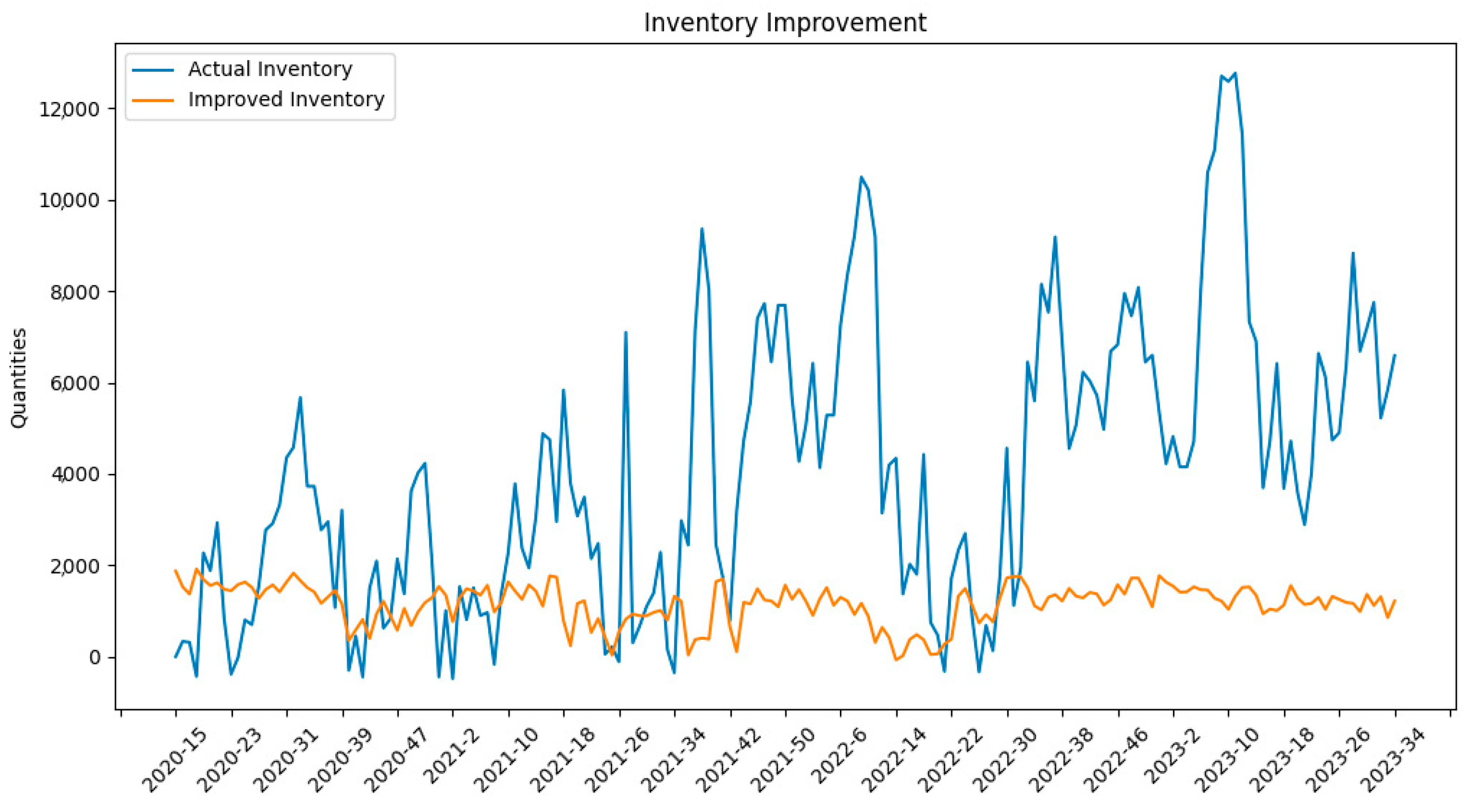
An important practical aspect of our work is evaluating how improved forecasting translates into better decision-making outcomes. To assess this, we carried out an inventory management simulation for the order dataset. We took the forecasting results of our model. We used them to drive an ordering policy for the manufacturer’s inventory and then compared inventory levels and stockout occurrences to the original scenario. As shown in Figure 8, our method effectively reduces overall inventory levels by about 80.62% compared to the original data without increasing stockouts. The stockout issue in the original data (where certain weeks had insufficient inventory to meet demand) is resolved within 12 weeks of applying our forecasting-based policy. The figure illustrates how inventory on hand evolves under the original vs. the new approach. Initially, both strategies start at the same inventory level; as our model’s order recommendations kick in, the inventory held begins to drop to a much lower trajectory while still covering the demand. By the end of the simulation period, the original system was carrying a large stock surplus, whereas our system maintained a leaner inventory that met all orders. This result is significant for the manufacturer—it implies that adopting our forecasting model to plan inventory could free up working capital tied in excess stock and reduce holding costs while avoiding the lost sales or disruption caused by stockouts.

For the order dataset (three-week ahead forecasting),

Table 12. Performance comparison of models on order dataset for forecasting three time points.

Models	Original			Our Method
	MAE	RMSE	R2	MAE	RMSE	R2
LSTM	741.8	935.2	−0.103	207.8	255.5	0.894
RNN	816.1	984.6	−0.276	221.4	273.2	0.888
GRU	776.4	933	−0.091	199.6	245.7	0.899
Seq2Seq	795.2	1022	−0.355	193.4	247.9	0.905
TCN	774.4	983.9	−0.178	206.6	225.2	0.916
Transformer	750.8	944.8	−0.073	190.7	232.0	0.926
Mamba	811.1	1003	−0.327	157.2	221.6	0.918
DLinear	741.1	964.3	−0.111	154.1	180.4	0.956

reports the performance. With the longer horizon, the error increases for all models (as expected), but our model’s performance degrades more gracefully compared to others. We attribute this to the decomposition effectively isolating trend and seasonality, and to the augmented features providing the model with richer information to handle multi-step dependencies.

For the electric load dataset (3-h ahead forecasting),

Table 13. Performance comparison of models on electric load dataset for forecasting three time points.

Models	Original			Our Method
	MAE	RMSE	R2	MAE	RMSE	R2
LSTM	21.34	27.00	0.407	3.573	4.700	0.982
RNN	19.83	24.76	0.499	5.228	6.220	0.968
GRU	21.50	26.57	0.424	5.279	7.025	0.959
Seq2Seq	21.66	27.56	0.383	4.084	5.408	0.976
TCN	21.76	27.35	0.391	8.179	10.51	0.909
Transformer	19.50	24.50	0.510	13.53	16.60	0.772
Mamba	19.58	24.64	0.505	6.289	8.196	0.945
DLinear	13.06	16.89	0.767	3.129	4.069	0.986

provides the results. As the horizon extends to 3 h, the errors increase relative to the 1-h case, but our decomposition-based model still maintains strong performance. It continues to outperform the baseline linear model and remains competitive with the more complex models at this intermediate horizon.

For the solar radiation dataset (3-h ahead forecasting),

Table 14. Performance comparison of models on solar radiation dataset for forecasting three time points.

Models	Original			Our Method
	MAE	RMSE	R2	MAE	RMSE	R2
LSTM	38.64	62.03	0.881	15.17	19.65	0.988
RNN	36.92	58.86	0.893	9.890	12.50	0.995
GRU	37.30	59.13	0.892	11.04	14.16	0.993
Seq2Seq	36.96	61.27	0.884	14.73	19.17	0.988
TCN	34.48	62.91	0.878	11.36	15.67	0.992
Transformer	48.68	69.78	0.850	13.82	18.58	0.989
Mamba	31.92	56.50	0.901	14.66	17.13	0.990
DLinear	38.20	60.21	0.888	8.517	11.30	0.996

shows the results. We observe the forecast error growing compared to the 1-h horizon, yet our method continues to exceed the baseline linear model’s accuracy. The performance remains strong given the nonlinear, short-cycle nature of the data, indicating the effectiveness of our decomposition and feature-engineering approach at this intermediate horizon.

For the order dataset (six-week ahead forecasting),

Table 15. Performance comparison of models on order dataset for forecasting six time points.

Models	Original			Our Method
	MAE	RMSE	R2	MAE	RMSE	R2
LSTM	801.2	1010.	−2.572	264.0	289.7	0.505
RNN	894.5	1094	−2.799	257.6	299.5	0.397
GRU	783.6	1009	−2.463	280.0	319.5	0.380
Seq2Seq	762.8	1001	−2.313	314.6	357.7	0.250
TCN	789.7	1052	−2.276	229.3	274.1	0.514
Transformer	854.5	1021	−2.642	218.5	268.9	0.706
Mamba	838.2	1048	−3.070	305.4	348.1	0.249
DLinear	825.6	1022	−2.928	177.0	235.4	0.727

shows the performance comparison. As expected, the prediction error further increases for all models at this longer horizon. Nonetheless, our model’s accuracy degrades more gracefully than the others, maintaining a relatively better R2 and lower error than the competing approaches at six weeks ahead.

For the electric load dataset (6-h ahead forecasting),

Table 16. Performance comparison of models on electric load dataset for forecasting six time points.

Models	Original			Our Method
	MAE	RMSE	R2	MAE	RMSE	R2
LSTM	20.42	26.22	0.457	5.248	6.665	0.962
RNN	19.38	24.40	0.528	6.090	7.585	0.951
GRU	19.87	25.36	0.489	6.999	8.681	0.937
Seq2Seq	21.24	27.29	0.415	5.034	6.513	0.964
TCN	28.49	35.65	−0.049	7.848	10.019	0.916
Transformer	28.15	35.57	−0.035	12.11	15.215	0.802
Mamba	21.10	25.81	0.475	5.414	6.888	0.960
DLinear	15.25	19.75	0.680	4.920	6.255	0.966

reports the results. At this longer horizon, all models experience higher errors; however, our model maintains a relatively low RMSE compared to the deep learning models. This highlights our model’s ability to capture the essential structure of the series, likely due to the explicit modeling of daily seasonality and trend components in the decomposition.

For the solar radiation dataset (6-h ahead forecasting),

Table 17. Performance comparison of models on solar radiation dataset for forecasting six time points.

Models	Original			Our Method
	MAE	RMSE	R2	MAE	RMSE	R2
LSTM	49.01	74.10	0.831	16.59	21.349	0.985
RNN	46.66	70.32	0.847	14.75	18.403	0.987
GRU	45.47	69.20	0.852	15.65	19.889	0.987
Seq2Seq	55.84	81.40	0.796	17.83	22.815	0.983
TCN	39.44	73.51	0.834	16.22	22.089	0.984
Transformer	48.03	74.07	0.830	36.38	41.333	0.947
Mamba	38.62	66.87	0.862	20.49	23.581	0.982
DLinear	44.63	69.36	0.851	14.56	18.394	0.989

shows the performance comparison. In this scenario, the gap between our linear model and the neural network models widens, suggesting that incorporating additional nonlinear components or exogenous variables might further improve performance for longer horizons on this dataset. Nonetheless, our method still outperforms the standard linear baseline and provides reasonable forecasts even at this challenging horizon, confirming that our approach is broadly effective across different types of time series.

Figure 8 shows an inventory level comparison before and after applying our forecasting method on the order dataset. The blue curve shows the original inventory levels over time (which are high and include some periods of stockouts), and the orange curve shows the improved inventory levels using our forecast-driven order recommendations. Our method keeps inventory much lower and more stable and, crucially, eliminates stockout events (weeks where inventory would drop to zero).

By quantitatively demonstrating improvements in an operational metric (inventory level), our forecasting approach’s benefits extend beyond error metrics—they can translate into tangible gains for business operations.

5. Conclusions and Future Work

In this work, we presented a linear model for time series forecasting that balances accuracy, interpretability, and efficiency. The model is built on a seasonal decomposition framework (using an additive model due to the stable seasonal patterns observed in the data) combined with an augmented-features generator and a gradient-based feature importance mechanism. Our results on three diverse datasets (product orders, machine energy load, and solar radiation) showed that this approach can achieve high forecasting accuracy on par with more complex models. The decomposition of time series into trend and seasonality allowed the linear model to focus on simplified sub-problems, while the augmented features captured additional structure (like acceleration/deceleration and frequency components) that further boosted performance. The gradient feature importance and elimination steps added interpretability and feature optimization, enabling the model to remain parsimonious without sacrificing predictive power.

We also demonstrated the practical impact of our method in a real-world scenario by showing significant improvements in inventory management when our forecasts are used for decision-making. This underscores the value of interpretable and reliable forecasting models in operational settings: not only can they produce accurate predictions, but they can do so in a way that stakeholders trust and act upon, leading to concrete benefits.

Despite these successes, there are several avenues for future work. First, while we adopted an additive decomposition model across all datasets (given that seasonal effects did not appear to scale with the series level in our cases), future research could explore adaptive or hybrid decomposition approaches that dynamically select between additive and multiplicative models based on data characteristics. For instance, a model could perform a preliminary check on seasonal variability and choose the decomposition type accordingly or even switch models if a time series exhibits regime changes in its seasonal behavior. Second, the current augmented feature set could be expanded with domain-specific features or nonlinear transformations. Although our linear model benefited from features capturing nonlinearity indirectly, another strategy is incorporating mild nonlinear modeling elements (like piecewise linear components or interactions between features) to handle patterns that pure linearity might miss. Third, our gradient-based importance method is well-suited to our linear model; applying similar ideas to more complex models (like neural networks) is not straightforward due to their nonlinear nature, so developing analogous interpretability techniques for deep time series models would be valuable. Finally, in our implementation, we trained the trend and seasonal forecasting models sequentially (one after the other). A possible improvement is to train or optimize them jointly or in parallel, which could reduce computation time and improve how the two components complement each other.

In conclusion, our study highlights that with thoughtful decomposition and feature engineering, simple linear models can offer a compelling blend of accuracy and interpretability for time series forecasting. By making model predictions more transparent and tying them to actionable insights (such as optimized inventory levels), we pave the way for broader acceptance and integration of advanced forecasting methods in industry practice. Future works will further bridge the gap between model complexity and interpretability, ensuring that improvements in predictive performance translate into real-world value.