Langlands Duality and Invariant Differential Operators

Abstract

Langlands duality is one of the most influential topics in mathematical research. It has many different appearances and influential subtopics. Yet there is a topic that until now has seemed unrelated to the Langlands program. That is the topic of invariant differential operators. It is strange since both items are deeply rooted in Harish-Chandra’s representation theory of semisimple Lie groups. In this paper we start building the bridge between the two programs. We first give a short review of our method of constructing invariant differential operators. A cornerstone in our program is the induction of representations from parabolic subgroups $P=MAN$ of semisimple Lie groups. The connection to the Langlands program is through the subgroup M, which other authors use in the context of the Langlands program. Next we consider the group $SL(2n,\mathbb{R})$, which is currently prominently used via Langlands duality. In that case, we have $M=SL(n,\mathbb{R})\times SL(n,\mathbb{R})$. We classify the induced representations implementing $P=MAN$. We find out and classify the reducible cases. Using our procedure, we classify the invariant differential operators in this case.

1. Introduction

In the last 50 years, Langlands duality has become one of the most influential topics in mathematical research [1,2]. It has many different appearances and influential subtopics, cf., an incomplete list: [3,4,5,6,7,8,9,10,11,12,13,14,15,16,17,18,19,20,21,22,23,24,25,26,27,28,29,30,31,32,33,34,35,36,37,38,39,40,41,42,43,44,45,46,47,48,49,50,51,52,53,54]. Note that some papers are written by authors who have created influential topics themselves. The last fact stresses the omnipresence of the Langlands program.

Yet, the concept of invariant differential operators has not been related to the Langlands program in the literature. That is strange, since both items are deeply rooted in Harish-Chandra’s representation theory of semisimple Lie groups. In this paper, we start building a bridge between the two programs.

Our attempt is based on our approach to the construction of invariant differential operators—for an exposition, we refer to [55], which is based also on many papers; see loc.cit. Our approach is deeply related to the Langlands general classification of representations of real semisimple groups G [2], taking into account the refinement by Knapp–Zuckermann [56].

One main ingredient in [2] is the parabolic subgroups $P=MAN$, such that M is a semisimple subgroup of our group G under study, A is an abelian subgroup, and N is a nilpotent subgroup preserved by the action A. Altogether, there is a local (Bruhat) decomposition of G using the subgroup $G^{\prime }=P\tilde{N}$, where $\tilde{N}$ is a nilpotent subgroup of G isomorphic to N also preserved by the action A, so that $G^{\prime }$ is dense in G. According to the construction of Langlands–Knapp–Zuckermann, every admissible irreducible representation of G may be obtained as a subrepresentation of representations of G induced by a representation of some P (some classes are enough—see details below).

Our construction of intertwining differential operators is based on the fact that the structure of parabolic subgroups is related to various subgroups of the Weyl groups $W({\mathcal{G}}^{\mathbb{C}},{\mathcal{H}}^{\mathbb{C}})$, where $\mathcal{G}$ is the Lie algebra of G, and $\mathcal{H}$ is the Cartan subalgebra of some $MA$. This is also related to various intertwining operators in the Langlands dual group, cf. [11,21].

Another aspect of the above is the Chevalley automorphism in the case of real groups, which is an exhibition of the local Langlands correspondence over R [3]. This is also related to the notion of Hermitian dual; see the case of $SL(n,\mathbb{R})$ below. Another application to representation theory using Heisenberg modules is done in [8].

Gauge theory aspects of the geometric Langlands program are studied in [31,33,42,51,54]. An exotic ’Chtoucas’ application of the Langlands program is given in [45]. Similarly, Langlands duality extends to Poisson–Lie duality via cluster theory [5]. Further, Langlands duality extends to representations of W-algebras in the quantum framework [6]. A proof of the global Langlands conjecture for GL(2) over a function field is given in [19].

Further, a two-parameter generalization of the geometric Langlands correspondence is proved for all simply laced Lie algebras [4]. This is related to two-parameter quantum groups, e.g., [55], and to 6d conformal supersymmetry [57]. The conformal case is also studied in [26]. The supersymmetry case is also studied in [7].

Various aspects of the Langlands program are given in [25]. The local Langlands correspondence is studied in [22,23]. Applications to integrability are shown in [18,24,29,52,53].

P.S. Some more recent references are added in [58,59,60,61,62,63,64,65].

Further, the present paper is organized as follows. In the next section, we give a synopsis of our approach. Then we apply this to the group $SL(2n,\mathbb{R})$, using the Langlands duality of the subgroup M used in the example. The cases $n=2,3,4$ are exposed in separate subsections.

2. Preliminaries

We start by giving a synopsis of our program of canonical construction of invariant differential operators.

Let G be a semisimple, non-compact Lie group, and K a maximal compact subgroup of G. Then, we have an Iwasawa decomposition $G=K{A}_0{N}_0$, where $A_0$ is an Abelian simply connected vector subgroup of G and $N_0$ is a nilpotent simply connected subgroup of G preserved by the action of $A_0$. Furthermore, let $M_0$ be the centralizer of $A_0$ in K. Then, the subgroup $P_0=M_0{A}_0{N}_0$ is a minimal parabolic subgroup of G. A parabolic subgroup $P^{\prime }=M^{\prime }{A}^{\prime }{N}^{\prime }$ is any subgroup of G which contains a minimal parabolic subgroup.

Furthermore, let $\mathcal{G},\mathcal{K},\mathcal{P},\mathcal{M},\mathcal{A},\mathcal{N}$ denote the Lie algebras of $G,K,P,M,A,N$, resp.

Further, for simplicity, we restrict it to maximal parabolic subgroups $P=MAN$, i.e., $\mathrm{rank}A=1$, resp., to maximal parabolic subalgebras $\mathcal{P}=\mathcal{M}\oplus \mathcal{A}\oplus \mathcal{N}$ with $dim\mathcal{A}=1$.

Let $\nu$ be a (non-unitary) character of A, $\nu \in {\mathcal{A}}^{*}$, parameterized by a real number d, called (for historical reasons) the conformal weight or energy.

Furthermore, let $\mu$ fix a discrete series representation $D^{\mu }$ of M on the Hilbert space $V_{\mu }$, or the finite-dimensional (non-unitary) representation of M with the same Casimirs.

We call the induced representation $\chi ={\mathrm{Ind}}_P^G(\mu \otimes \nu \otimes 1)$ an elementary representation of G [66]. (These are called generalized principal series representations (or limits thereof) in [67]). Their spaces of functions are

$${\mathcal{C}}_{\chi }=\{\mathcal{F}\in C^{\infty }(G,V_{\mu })|\mathcal{F}\left(gman\right)=e^{-\nu \left(H\right)}·D^{\mu }\left(m^{-1}\right)\mathcal{F}\left(g\right)\}$$

(1)

where $a=exp\left(H\right)\in A^{\prime }$, $H\in {\mathcal{A}}^{\prime }$, $m\in M^{\prime }$, $n\in N^{\prime }$. The representation action is the left regular action:

$$\left({\mathcal{T}}^{\chi }\left(g\right)\mathcal{F}\right)\left(g^{\prime }\right)=\mathcal{F}\left(g^{-1}{g}^{\prime }\right),g,g^{\prime }\in G.$$

(2)

An important ingredient in our considerations is the highest/lowest-weight representations of ${\mathcal{G}}^{\mathbb{C}}$. These can be realized as (factor-modules of) Verma modules $V^{Ł}$ over ${\mathcal{G}}^{\mathbb{C}}$, where $Ł\in {\left({\mathcal{H}}^{\mathbb{C}}\right)}^{*}$, ${\mathcal{H}}^{\mathbb{C}}$ is a Cartan subalgebra of ${\mathcal{G}}^{\mathbb{C}}$ and the weight $Ł=Ł\left(\chi \right)$ is determined uniquely from $\chi$ [55].

Actually, since our ERs may be induced from finite-dimensional representations of $\mathcal{M}$ (or their limits), the Verma modules are always reducible. Thus, it is more convenient to use generalized Verma modules ${\tilde{V}}^{Ł}$ such that the role of the highest/lowest-weight vector $v_0$ is taken by the (finite-dimensional) space $V_{\mu }{v}_0$. For the generalized Verma modules (GVMs), the reducibility is controlled only by the value of the conformal weight d. Relatedly, for the intertwining differential operators, only the reducibility with regard to non-compact roots is essential.

Another main ingredient of our approach is as follows. We group the (reducible) ERs with the same Casimirs in sets called multiplets [55]. The multiplet corresponding to fixed values of the Casimirs may be depicted as a connected graph, the vertices of which correspond to the reducible ERs, and the lines (arrows) between the vertices correspond to intertwining operators. The explicit parameterization of the multiplets and of their ERs is important in understanding the situation. The notion of multiplets was introduced in [68] and applied to representations of $S{O}_o(p,q)$ and $SU(2,2)$, resp., induced from their minimal parabolic subalgebras. Then it was applied to the conformal superalgebra [69], to quantum groups, and to infinite-dimensional (super)algebras; see later volumes of [55].

In fact, the multiplets contain explicitly all the data necessary to construct the intertwining differential operators. Actually, the data for each intertwining differential operator consist of the pair ($\beta$,m), where $\beta$ is a (non-compact) positive root of ${\mathcal{G}}^{\mathbb{C}}$, $m\in \mathbb{N}$, such that the BGG Verma module reducibility condition (for the highest-weight modules) is fulfilled:

$$(Ł+\rho ,{\beta }^{\vee })=m,{\beta }^{\vee }\equiv 2\beta /(\beta ,\beta )$$

(3)

where $\rho$ is half the sum of the positive roots of ${\mathcal{G}}^{\mathbb{C}}$. When the above holds, then the Verma module with shifted weight $V^{Ł-m\beta }$ (or ${\tilde{V}}^{Ł-m\beta }$ for GVM and $\beta$ non-compact) is embedded in the Verma module $V^{Ł}$ (or ${\tilde{V}}^{Ł}$). This embedding is realized by a singular vector $v_s$ determined by a polynomial ${\mathcal{P}}_{m,\beta }\left({\mathcal{G}}^{-}\right)$ in the universal enveloping algebra $\left(U\left({\mathcal{G}}_{-}\right)\right)v_0$, and ${\mathcal{G}}^{-}$ is the subalgebra of ${\mathcal{G}}^{\mathbb{C}}$ generated by the negative root generators [70]. More explicitly [55], $v_{m,\beta }^s={\mathcal{P}}_{m,\beta }{v}_0$ (or $v_{m,\beta }^s={\mathcal{P}}_{m,\beta }{V}_{\mu }{v}_0$ for GVMs). Then, there exists an [55] intertwining differential operator

$${\mathcal{D}}_{m,\beta }:{\mathcal{C}}_{\chi \left(Ł\right)}⟶{\mathcal{C}}_{\chi (Ł-m\beta )}$$

(4)

given explicitly by

$${\mathcal{D}}_{m,\beta }={\mathcal{P}}_{m,\beta }\left(\widehat{{\mathcal{G}}^{-}}\right)$$

(5)

where $\widehat{{\mathcal{G}}^{-}}$ denotes the right action on the function $\mathcal{F}$.

3. Main Results

3.1. Restricted Weyl Groups and Related Notions

In our exposition below, we shall use the so-called Dynkin labels:

$$m_i\equiv (Ł+\rho ,{\alpha }_i^{\vee }),i=1,\dots ,n,$$

(6)

where $Ł=Ł\left(\chi \right)$, $\rho$ is half the sum of the positive roots of ${\mathcal{G}}^{\mathbb{C}}$.

We shall also use the so-called Harish–Chandra parameters:

$$m_{\beta }\equiv (Ł+\rho ,{\beta }^{\vee }),$$

(7)

where $\beta$ is any positive root of ${\mathcal{G}}^{\mathbb{C}}$. These parameters are redundant, since they are expressed in terms of the Dynkin labels; however, some statements are best formulated in their terms. (Clearly, both the Dynkin labels and Harish–Chandra parameters have their origin in the BGG reducibility condition (3)).

Next, we recall the action of the Weyl group on highest weights:

$$w_{\beta }\left(Ł\right)\doteq Ł-(Ł+\rho ,{\beta }^{\vee })\beta$$

(8)

and thus,

$$w_{\beta }\left(Ł\right)=Ł-m_{\beta }\beta$$

(9)

and the shifted weight in (4) results by the action of the Weyl group as in (9).

Next, we mention the important notion of restricted Weyl group. We first need the so-called restricted roots.

Let ${\Delta }_{{\mathcal{A}}^{\prime }}$ be the restricted root system of $(\mathcal{G},{\mathcal{A}}^{\prime })$:

$$\begin{array}{c}{\Delta }_{{\mathcal{A}}^{\prime }}\doteq \{\lambda \in {\mathcal{A}}^{\prime *}|\lambda \ne 0,{\mathcal{G}}_{{\mathcal{A}}^{\prime }}^{\lambda }\ne 0\},\hfill \\ {\mathcal{G}}_{{\mathcal{A}}^{\prime }}^{\lambda }\doteq \{X\in \mathcal{G}|[Y,X]=\lambda \left(Y\right)X,\forall Y\in {\mathcal{A}}^{\prime }\}.\hfill \end{array}$$

(10)

The elements of ${\Delta }_{{\mathcal{A}}^{\prime }}$ are called ${\mathcal{A}}^{\prime }$-restricted roots.

[The terminology comes from the fact that things may be arranged so that these roots are obtained as a restriction to ${\mathcal{A}}^{\prime }$ of some roots of the root system $\Delta$ of the pair $({\mathcal{G}}^{\mathbb{C}},{\mathcal{H}}^{\mathbb{C}})$.]

For $\lambda \in {\Delta }_{{\mathcal{A}}^{\prime }}$, ${\mathcal{G}}_{{\mathcal{A}}^{\prime }}^{\lambda }$ are called ${\mathcal{A}}^{\prime }$-restricted root spaces, ${\dim }_R{\mathcal{G}}_{{\mathcal{A}}^{\prime }}^{\lambda }\ge 1$.

Next we introduce some ordering (e.g., the lexicographic one) in ${\Delta }_{{\mathcal{A}}^{\prime }}$. Accordingly, the latter is split into positive and negative restricted roots: ${\Delta }_{{\mathcal{A}}^{\prime }}={\Delta }_{{\mathcal{A}}^{\prime }}^{+}\cup {\Delta }_{{\mathcal{A}}^{\prime }}^{-}$.

Furthermore, we introduce the simple restricted root system ${\Delta }_{{\mathcal{A}}^{\prime }}^R$, which is the simple root system of the restricted roots. Next we introduce the restricted Weyl reflections: for each root $\lambda \in {\Delta }_{{\mathcal{A}}^{\prime }}^{+}$ we define a reflection $s_{\lambda }$ in ${{\mathcal{A}}^{\prime }}^{*}$:

$$s_{\lambda }\left(\mu \right)\equiv \mu -2{\displaystyle \frac{(\lambda ,\mu )}{(\lambda ,\lambda )}}\lambda ,\mu \in {{\mathcal{A}}^{\prime }}^{*}$$

(11)

Clearly, $s_{\lambda }\left(\lambda \right)=-\lambda$, $s_{\lambda }^2={\mathrm{id}}_{{{\mathcal{A}}^{\prime }}^{*}}$.

The above reflections generate the ${\mathcal{A}}^{\prime }$-restricted Weyl group $W(\mathcal{G},{\mathcal{A}}^{\prime })$.

The above may be applied to the case when, instead of some ${\mathcal{A}}^{\prime }$, we use an arbitrary subalgebra ${\mathcal{H}}^{\prime }$ of $\mathcal{H}$.

3.2. The Case of $SL(2n,\mathbb{R})$

In this paper, we treat the case of $G=SL(2n,\mathbb{R})$, $\mathcal{G}=sl(2n,\mathbb{R})$. We restrict it to maximal parabolic subalgebra

$$\begin{array}{ccc}\mathcal{P}\hfill & =& \mathcal{M}\oplus \mathcal{A}\oplus \mathcal{N}\hspace{1em}\hspace{1em}\hspace{1em}\hspace{1em}\hspace{1em}\hspace{1em}\hspace{1em}\hspace{1em}\hspace{1em}\hspace{1em}\hspace{1em}\hspace{1em}\hspace{1em}\hfill \end{array}$$

(12)

$$\begin{array}{ccc}\hfill \mathcal{M}& =& sl(n,\mathbb{R})\oplus sl(n,\mathbb{R}),dim\mathcal{A}=1,dim\mathcal{N}=n^2\hfill \end{array}$$

(13)

In the context of relative Langlands duality, this case was studied in, e.g., [10], as the subcase of hyperspherical dual pairs [71]. There, the relation to physics appeared as an arithmetic analog of the electric–magnetic duality of boundary conditions in the four-dimensional supersymmetric Yang–Mills theory. This aspect will be recovered for $n=2$ below.

In this section, we start with $G=SL(m,\mathbb{R})$, the group of invertible $m\times m$ matrices with real elements and determinant 1. Then $\mathcal{G}=sl(m,\mathbb{R})$, and the Cartan involution is given explicitly by $\tilde{h}X=-{}^{t}X$, where ${}^{t}X$ is the transpose of $X\in \mathcal{G}$. Thus, $\mathcal{K}\cong so\left(m\right)$, and is spanned by the matrices (r.l.s. stands for real linear span)

$$\mathcal{K}=\mathrm{r}.\mathrm{l}.\mathrm{s}.\{X_{ij}\equiv e_{ij}-e_{ji},1\le i<j\le m\},$$

(14)

where $e_{ij}$ are the standard matrices with only nonzero entry (=1) on the i-th row and j-th column, ${\left(e_{ij}\right)}_{k\ell }={\delta }_{ik}{\delta }_{j\ell }$. (Note that $\mathcal{G}$ does not have discrete series representations if $m>2$.)

Further, the complementary space $\mathcal{P}$ is given by

$$\begin{array}{ccc}\hfill \mathcal{P}& =& \mathrm{r}.\mathrm{l}.\mathrm{s}.\{Y_{ij}\equiv e_{ij}+e_{ji},1\le i<j\le m,\hfill \end{array}$$

(15)

$$\begin{array}{c}\hspace{1em}\hspace{1em}\hspace{1em}{H}_j\equiv e_{jj}-e_{j+1,j+1},1\le j\le m-1\}.\hfill \end{array}$$

(16)

The split rank is $r=m-1$, and from (15) it is obvious that in this setting one has

$$\mathcal{H}=\mathrm{r}.\mathrm{l}.\mathrm{s}.\{H_j,1\le j\le n-1=r\}.$$

(17)

The simple root vectors are given explicitly by

$$X_j^{+}\doteq e_{j,j+1},X_j^{-}\doteq e_{j+1,j},1\le j\le m-1.$$

(18)

Note that matters are arranged so that

$$[X_j^{+},X_j^{-}]=H_j,[H_j,X_j^{\pm }]=\pm 2X_j^{\pm },$$

(19)

and further we shall denote by $sl{(2,\mathbb{R})}_j$ the $sl(2,\mathbb{R})$ subalgebra of $\mathcal{G}$ spanned by $X_j^{\pm },H_j$.

In our case of consideration, $m=2n$, we have

$$\mathcal{M}=sl\left(n\right)\oplus sl\left(n\right)$$

(20)

and we use representations of $\mathcal{M}$ indexed as follows:

$$\widehat{\mathcal{M}}=(m_1,\dots ,m_{n-1};m_{n+1},\dots ,m_{2n-1})$$

(21)

When all $m_j$ are natural numbers, $\widehat{\mathcal{M}}$ indexes the unitary finite-dimensional irreps of $\mathcal{M}$.

3.3. $sl\left(4\right)$

In the case of $sl\left(4\right)$, the parabolic $\mathcal{M}$ factor is

$${\mathcal{M}}_4=sl\left(2\right)\oplus sl\left(2\right)$$

(22)

the representations being indexed by the numbers $m_1,m_3$.

Relatedly, the representations of $\mathcal{G}$ are indexed by

$${\chi }_4=[m_1,m_2,m_3]$$

(23)

It is well-known that when all $m_j$ are natural numbers, ${\chi }_4$ exhausts the finite-dimensional representations of $\mathcal{G}$. Each representation ${\chi }_4$ is part of 24-member multiplet naturally corresponding to the 24 elements of the Weyl group of $sl\left(4\right)$. When we consider induction from ${\mathcal{M}}_4$, we have six-member multiplets (sextets) parametrized as follows:

$$\begin{array}{ccc}\hfill {\chi }^{-}& =& \{m_1,m_2,m_3\},\hfill \\ \hfill {\chi }^{\prime -}& =& \{m_{12},-m_2,m_{23}\},{Ł}^{\prime -}={Ł}^{-}-m_2{\alpha }_2\hfill \\ \hfill {\chi }^{″-}& =& \{m_2,-m_{12},m_{13}\},{Ł}^{″-}={Ł}^{\prime -}-m_1{\alpha }_{12}\hfill \\ \hfill {\chi }^{″+}& =& \{m_{13},-m_{23},m_2\},{Ł}^{″+}={Ł}^{\prime -}-m_3{\alpha }_{23}\hfill \\ \hfill {\chi }^{\prime +}& =& \{m_{23},-m_{13},m_{12}\},{Ł}^{\prime +}={Ł}^{″-}-m_3{\alpha }_{23}={Ł}^{″+}-m_1{\alpha }_{12}\hfill \\ \hfill {\chi }^{+}& =& \{m_3,-m_{13},m_1\},{Ł}^{+}={Ł}^{\prime +}-m_2{\alpha }_2\hfill \end{array}$$

(24)

where $m_{12}\equiv m_1+m_2$, $m_{23}\equiv m_2+m_3$, $m_{13}\equiv m_1+m_2+m_3$. Note that the ± pairs are related by Knapp–Stein [72] integral intertwining operators $G^{\pm }$ so that the operators $G^{+}$ act from ${\chi }^{-}$ to ${\chi }^{+}$, while $G^{-}$ act from ${\chi }^{+}$ to ${\chi }^{-}$, etc.

Thus, the Knapp–Stein duality is a manifestation of the Langlands duality.

We recall the number $N_M$ of ERs in a multiplet corresponding to induction from a parabolic given by [55]

$$N_M={\displaystyle \frac{\left|W\right(\mathcal{G},\mathcal{H}\left)\right|}{\left|W\right(\mathcal{M},{\mathcal{H}}_m\left)\right|}}$$

(25)

which in our case ($\mathcal{M}={\mathcal{M}}_4$) gives

$$N_M={\displaystyle \frac{24}{4}}=6.$$

(26)

This is what we have obtained.

An alternative parametrization stressing the duality is given as follows:

$$\begin{array}{ccc}\hfill {\chi }^{\pm }& =& \{{(m_1;m_3)}^{\pm };c=\pm (m_2+\frac{1}{2}(m_1+m_3))\},\hfill \\ \hfill {\chi }^{\prime \pm }& =& \{{(m_{12},m_{23})}^{\pm };c=\pm \frac{1}{2}(m_1+m_3)\},\hfill \\ \hfill {\chi }^{″\pm }& =& \{{(m_2,m_{13})}^{\pm };c=\pm \frac{1}{2}(m_1-m_3)\},\hfill \end{array}$$

where ${(p;q)}^{+}=(q;p)$, ${(p;q)}^{-}=(p;q)$,

The irreducible subrepresentations $\mathcal{E}$ of ${\chi }^{-}$ are finite-dimensional, exhausting all finite-dimensional (non-unitary) representations of $sl\left(4\right)$, and of all real forms.

Note also that the dimensions of the ±-inducing pair of $\mathcal{M}$ are the same, namely, $m_1{m}_3$ for ${\chi }^{\pm }$, $m_{12}{m}_{23}$ for ${\chi }^{\prime \pm }$, and $m_2{m}_{13}$ for ${\chi }^{\prime \prime \pm }$.

Finally, we use the simplest case $m_1=m_2=m_3=1$ to exhibit the electro-magnetic duality which has transparent physical meaning for the conformal real form $su(2,2)$. The multiplet is depicted on Figure 1 (complete treatment may be found in [55]).

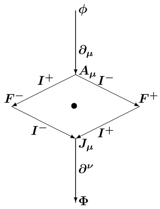
Figure 1. Simplest case of conformal invariant differential operators $F^{\pm }$ depict the duality decomposition of the electromagnetic eld $F_{\mu v}$. $A_{\mu }$, resp., $J_{\mu }$, is the electromagnetic potential, resp., the current. $I^{\pm }$ depict the differential operators which come from the equation ${\partial }_{\left[\mu Av\right]=F_{\mu v}}$. Knapp-Stein operators relate cases symmetric w.r.t. the central black dot.

Multiplets containing the finite-dimensional subrepresentations are called main multiplets. The other multiplets are called reduced multiplets. These contain inducing finite-dimensional representations of $\mathcal{M}$.

In the case at hand, there are three such cases so that each is a doublet (containing two ERs). Explicitly, the three cases are

$$\begin{array}{ccc}\hfill {\chi }_1^{\pm }& =& \{{(m_2,m_{23})}^{\pm };c=\pm \frac{1}{2}{m}_3\},{Ł}_1^{+}={Ł}_1^{-}-m_3{\alpha }_{23}\hfill \end{array}$$

(27a)

$$\begin{array}{ccc}\hfill {\chi }_2^{\pm }& =& \{{(m_1;m_3)}^{\pm };c^{\pm }=\pm \frac{1}{2}(m_1+m_3)\},\hspace{1em}\hspace{1em}\hspace{1em}\hspace{1em}\hfill \end{array}$$

(27b)

$$\begin{array}{ccc}\hfill {\chi }_3^{\pm }& =& \{{(m_{12},m_2)}^{\pm };c=\pm \frac{1}{2}{m}_1\},{Ł}_3^{+}={Ł}_3^{-}-m_1{\alpha }_{12}\hfill \end{array}$$

(27c)

Note that here the invariant operators are deformations of the Knapp–Stein integral operators from the sextet picture. Thus, those from ${\chi }^{+}$ to ${\chi }^{-}$ are still integral operators, while those from ${\chi }^{-}$ to ${\chi }^{+}$ are differential operators via degeneration of the Knapp–Stein integral operators. Yet, in the first and third case, these are differential operators inherited from the sextets, and only the operators in (27b) from ${\chi }_2^{-}$ to ${\chi }_2^{+}$ are obtained due to genuine degeneration of the Knapp–Stein integral operators [55]. This is the standard degeneration of the two-point function-kernel, which at the reducibility points is a generalized function with regularization, turning it into delta-function (cf. Gelfand et al. [73]). Finally, we add that in the case $m_1=m_3=n$ the operators (27b), which become a degree of the d’Alembert operator

$${\mathcal{D}}_{n,n}=const{☐}^{c^{+}}=const{☐}^n$$

(28)

3.4. $sl\left(6\right)$

Here, we take up the case $sl\left(6\right)$ with the parabolic $\mathcal{M}$ factor

$${\mathcal{M}}_5=sl(3,\mathbb{R})\oplus sl(3,\mathbb{R})={\mathcal{M}}_{2L}\oplus {\mathcal{M}}_{2R}$$

(29)

We start with elementary representations of $sl(6,\mathbb{R})$ indexed by five numbers

$$\chi =\{m_1,m_2,m_3,m_4,m_5\},$$

(30)

so that $m_1,m_2$ index the representations of ${\mathcal{M}}_{2L}$, $m_4,m_5$ index the representations of ${\mathcal{M}}_{2R}$, while $m_3$ indexes the representations of the dilatation subalgebra $\mathcal{A}$.

When all $m_j$ are positive integers, we use Formula (25) so we have a multiplet of 20 members, since

$$N_M={\displaystyle \frac{\left|W\right(\mathcal{G},\mathcal{H}\left)\right|}{\left|W\right({\mathcal{M}}_5,{\mathcal{H}}_5\left)\right|}}={\displaystyle \frac{6!}{{(3!)}^2}}=20.$$

(31)

Theorem 1.

The signatures of the reducible induced representations are

$$\begin{array}{c}{\chi }_1=\{m_1,m_2,m_3,m_4,m_5\},\hfill \\ {\chi }_2=\{m_1,m_{23},-m_3,m_{34},m_5\},{Ł}_2={Ł}_1-m_3{\alpha }_3\hfill \\ {\chi }_3=\{m_{12},m_3,-m_{23},m_{24},m_5\},{Ł}_3={Ł}_2-m_2{\alpha }_{23}\hfill \\ {\chi }_4=\{m_1,m_{24},-m_{34},m_3,m_{45}\},{Ł}_4={Ł}_2-m_4{\alpha }_{34}\hfill \\ {\chi }_5=\{m_2,m_3,-m_{13},m_{14},m_5\},{Ł}_5={Ł}_3-m_1{\alpha }_{13}\hfill \\ {\chi }_6=\{m_{12},m_{34},-m_{24},m_{23},m_{45}\},{Ł}_6={Ł}_3-m_4{\alpha }_{34}\hfill \\ {\chi }_7=\{m_1,m_{25},-m_{35},m_3,m_4\},{Ł}_7={Ł}_4-m_5{\alpha }_{35}\hfill \\ {\chi }_8=\{m_2,m_{34},-m_{14},m_{13},m_{45}\},{Ł}_8={Ł}_6-m_1{\alpha }_{13}\hfill \\ {\chi }_9=\{m_{13},m_4,-m_{24},m_2,m_{35}\},{Ł}_9={Ł}_6-m_3{\alpha }_{24}\hfill \\ {\chi }_{10}=\{m_{12},m_{35},-m_{25},m_{23},m_4\},{Ł}_{10}={Ł}_6-m_5{\alpha }_{35}\hfill \\ {\chi }_{11}=\{m_{23},m_4,-m_{14},m_{12},m_{35}\},{Ł}_{11}={Ł}_8-m_3{\alpha }_{24}\hfill \\ {\chi }_{12}=\{m_2,m_{35},-m_{15},m_{13},m_4\},{Ł}_{12}={Ł}_8-m_5{\alpha }_{35}\hfill \\ {\chi }_{13}=\{m_{13},m_{45},-m_{25},m_2,m_{34}\},{Ł}_{13}={Ł}_{10}-m_3{\alpha }_{24}\hfill \\ {\chi }_{14}=\{m_3,m_4,-m_{14},m_1,m_{25}\},{Ł}_3={Ł}_{11}-m_2{\alpha }_{14}\hfill \\ {\chi }_{15}=\{m_{23},m_{45},-m_{15},m_{12},m_{34}\},{Ł}_{15}={Ł}_{11}-m_5{\alpha }_{35}\hfill \\ {\chi }_{16}=\{m_{14},m_5,-m_{25},m_2,m_3\},{Ł}_{13}={Ł}_{10}-m_4{\alpha }_{25}\hfill \\ {\chi }_{17}=\{m_3,m_{45},-m_{15},m_1,m_{24}\},{Ł}_{17}={Ł}_{15}-m_2{\alpha }_{14}\hfill \\ {\chi }_{18}=\{m_{24},m_5,-m_{15},m_{12},m_3\},{Ł}_{18}={Ł}_{15}-m_4{\alpha }_{25}\hfill \\ {\chi }_{19}=\{m_{34},m_5,-m_{15},m_1,m_{23}\},{Ł}_{19}={Ł}_{17}-m_4{\alpha }_{25}\hfill \\ {\chi }_{20}=\{m_4,m_5,-m_{15},m_1,m_2\},{Ł}_{20}={Ł}_{19}-m_3{\alpha }_{15}\hfill \end{array}$$

(32)

Proof. 

The Proof is constructive. We start with the representation ${\chi }_1$; then, by our procedure, we find the embedded representation ${\chi }_2$. Then from the latter we find the embedded representations ${\chi }_3$ and ${\chi }_4$. We proceed to the last case ${\chi }_{20}$, which is reducible only by the Knapp–Stein operator intertwining it with its Langlands dual ${\chi }_1$. □

Note that we have indicated some embeddings between the representations, but not all in order not to clutter the formulae. The full picture is seen in Figure 2.

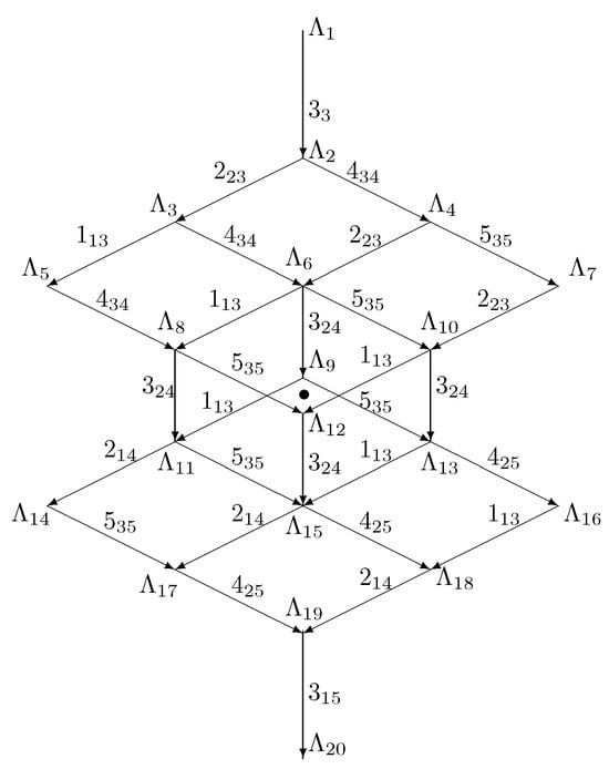
Figure 2. Main multiplets for $sl(6,\mathbb{R})$.

We quickly observe that the representations ${\chi }_n$ and ${\chi }_{21-n}$ are Langlands duals related by Knapp–Stein operators. More explicitly, this duality is given by the following presentation of the same multiplet:

$$\begin{array}{c}{\chi }_1^{\pm }=\{{(m_1,m_2;m_4,m_5)}^{\pm };c=\pm (m_3+\frac{1}{2}{m}_{12,45})\},\hfill \\ {\chi }_2^{\pm }=\{{(m_1,m_{23};m_{34},m_5)}^{\pm };c=\pm \frac{1}{2}{m}_{12,45}\},\hfill \\ {\chi }_3^{\pm }=\{{(m_{12},m_3;m_{24},m_5)}^{\pm };c=\pm \frac{1}{2}{m}_{1,45}\},\hfill \\ {\chi }_4^{\pm }=\{{(m_1,m_{24};m_3,m_{45})}^{\pm };c=\pm \frac{1}{2}{m}_{12,5}\},\hfill \\ {\chi }_5^{\pm }=\{{(m_2,m_3;m_{14},m_5)}^{\pm };c=\pm \frac{1}{2}(m_{45}-m_1)\},\hfill \\ {\chi }_6^{\pm }=\{{(m_{12},m_{34};m_{23},m_{45})}^{\pm };c=\pm \frac{1}{2}(m_1+m_5)\},\hfill \\ {\chi }_7^{\pm }=\{{(m_1,m_{25};m_3,m_4)}^{\pm };c=\pm \frac{1}{2}(m_{12}-m_5)\},\hfill \\ {\chi }_8^{\pm }=\{{(m_2,m_{34};m_{13},m_{45})}^{\pm };c=\pm \frac{1}{2}(m_5-m_1)\},\hfill \\ {\chi }_9^{\pm }=\{{(m_{13},m_4;m_2,m_{35})}^{\pm };c=\pm \frac{1}{2}(m_1+m_5)\},\hfill \\ {\chi }_{10}^{\pm }=\{{(m_{12},m_{35};m_{23},m_4)}^{\pm };c=\pm \frac{1}{2}(m_1-m_5)\},\hfill \end{array}$$

(33)

where ${(p,q;r,s)}^{+}\equiv (r,s;p,q)$, ${(p,q;r,s)}^{-}\equiv (p,q;r,s)$, and the inducing number of the dilatation subalgebra $\mathcal{A}$ is replaced by the conformal factor c. Clearly, ${\chi }_n^{-}={\chi }_n$, ${\chi }_n^{+}={\chi }_{21-n}$ for $1\le n\le 10$.

3.5. Reduced Multiplets

Here, we just list the reduced multiplets which contain finite-dimensional irreps of the inducing $\mathcal{M}$.

$$\begin{array}{ccc}& 1& {\chi }_3^{\prime \pm }=\{{(m_2,m_3;m_{24},m_5)}^{\pm };c=\pm \frac{1}{2}{m}_{45}\},\hfill \\ & & {\chi }_6^{\prime \pm }=\{{(m_2,m_{34};m_{23},m_{45})}^{\pm };c=\pm \frac{1}{2}{m}_5\},\hfill \\ & & {\chi }_9^{\prime \pm }=\{{(m_{23},m_4;m_2,m_{35})}^{\pm };c=\pm \frac{1}{2}{m}_5\},\hfill \\ & 13& {\chi }_6^{″\pm }=\{{(m_2,m_4;m_2,m_{45})}^{\pm };c=\pm \frac{1}{2}{m}_5\},\hfill \\ & 14& {\chi }_3^{″\pm }=\{{(m_2,m_3;m_{23},m_5)}^{\pm };c=\pm \frac{1}{2}{m}_5\},\hfill \end{array}$$

(34a)

$$\begin{array}{cc}15& {\chi }_9^{″\pm }=\{{(m_{23},m_4;m_2,m_{34})}^{\pm };c=0\},\hspace{1em}\hfill \end{array}$$

(34b)

$$\begin{array}{cc}135& {\chi }_6=\{(m_2,m_4;m_2,m_4);c=0\},\hspace{1em}\hspace{1em}\hfill \end{array}$$

(34c)

$$\begin{array}{cc}2& {\chi }_2^{\prime \pm }=\{{(m_1,m_3;m_{34},m_5)}^{\pm };c=\pm \frac{1}{2}{m}_{1,45}\},\hfill \\ & {\chi }_4^{\prime \pm }=\{{(m_1,m_{34};m_3,m_{45})}^{\pm };c=\pm \frac{1}{2}{m}_{1,5}\},\hfill \\ & {\chi }_7^{\prime \pm }=\{{(m_1,m_{35};m_3,m_4)}^{\pm };c=\pm \frac{1}{2}(m_1-m_5)\},\hfill \\ 24& {\chi }_2^{″\pm }=\{{(m_1,m_3;m_3,m_5)}^{\pm };c=\pm \frac{1}{2}{m}_{1,5}\},\hfill \\ 25& {\chi }_4^{″\pm }=\{{(m_1,m_{34};m_3,m_4)}^{\pm };c=\pm \frac{1}{2}{m}_1\},\hfill \end{array}$$

(35)

$$\begin{array}{cc}3& {\chi }_1^{\prime \pm }=\{{(m_1,m_2;m_4,m_5)}^{\pm };c=\pm \frac{1}{2}{m}_{12,45}\},\hfill \\ & {\chi }_6^{\prime \pm }=\{{(m_{12},m_4;m_2,m_{45})}^{\pm };c=\pm \frac{1}{2}{m}_{1,5}\},\hfill \\ & {\chi }_8^{\prime \pm }=\{{(m_2,m_4;m_{12},m_{45})}^{\pm };c=\pm \frac{1}{2}(m_5-m_1)\},\hfill \end{array}$$

(36)

Note that the numbers on the left indicate which representation numbers are missing in the displayed signatures.

Further, note that the ± pairs are Knapp–Stein pairs, except (34b), where the operator is just a flip of the finite-dimensional inducing irreps. Note also that the case (34c) is a singlet.

Note that we do not display reduced multiplets with the missing labels $m_4$ and $m_5$ since due to duality they are equivalent to multiplets with missing labels $m_2$, $m_1$, resp.

4. Case sl(8)

Here we consider the case $sl\left(8\right)$ with the parabolic $\mathcal{M}$ factor

$${\mathcal{M}}_7=sl(4,\mathbb{R})\oplus sl(4,\mathbb{R})={\mathcal{M}}_{2L}\oplus {\mathcal{M}}_{2R}$$

(37)

Analogously to the previously considered cases, the representations of $sl(8,\mathbb{R})$ are indexed by seven numbers

$$\chi =\{m_1,m_2,m_3,m_4,m_5,m_6,,m_7\},$$

(38)

so that $m_1,m_2,m_3$ index the representations of ${\mathcal{M}}_{2L}$, $m_5,m_6,m_7$ index the representations of ${\mathcal{M}}_{2R}$, and $m_4$ indexes the representations of the dilatation subalgebra $\mathcal{A}$.

When all $m_j$ are positive integers, we again use the formula (25) so we have a multiplet of 70 members, since

$$N_M={\displaystyle \frac{\left|W\right(\mathcal{G},\mathcal{H}\left)\right|}{\left|W\right({\mathcal{M}}_7,{\mathcal{H}}_7\left)\right|}}={\displaystyle \frac{8!}{{(4!)}^2}}=70.$$

(39)

Theorem 2.

The signatures of the reducible induced representations using only the Knapp–Stein dual signatures are

$$\begin{array}{c}{\chi }_1^{\pm }=\{{(m_1,m_2,m_3,m_4,m_5,m_6,m_7)}^{\pm },c^{\pm }=\pm (m_4+\frac{1}{2}{m}_{13,57})\},\hfill \\ {\chi }_2^{\pm }=\{{(m_1,m_2,m_{34},-m_4,m_{45},m_6,m_7)}^{\pm },c^{\pm }=\pm \left(\frac{1}{2}{m}_{17}\right)\}\hfill \\ {\chi }_3^{\pm }=\{{(m_1,m_{23},m_4,-m_{34},m_{35},m_6,m_7)}^{\pm },c^{\pm }=\pm \left(\frac{1}{2}{m}_{12,57}\right)\}\hfill \\ {\chi }_4^{\pm }=\{{(m_1,m_2,m_{35},-m_{45},m_4,m_{56},m_7)}^{\pm },c^{\pm }=\pm \left(\frac{1}{2}{m}_{13,67}\right)\}\hfill \\ {\chi }_5^{\pm }=\{{(m_{12},m_3,m_4,-m_{24},m_{25},m_6,m_7)}^{\pm },c^{\pm }=\pm \left(\frac{1}{2}{m}_{1,57}\right)\}\hfill \\ {\chi }_6^{\pm }=\{{(m_1,m_{23},m_{45},-m_{35},m_{34},m_{56},m_7)}^{\pm },c^{\pm }=\pm \left(\frac{1}{2}{m}_{12,67}\right)\}\hfill \\ {\chi }_7^{\pm }=\{{(m_1,m_2,m_{36},-m_{46},m_4,m_5,m_{67})}^{\pm },c^{\pm }=\pm \left(\frac{1}{2}{m}_{13,7}\right)\}\hfill \\ {\chi }_8^{\pm }=\{(m_2,m_3,m_4,-m_{14}{(m_{15},m_{56},m_7)}^{\pm },c^{\pm }=\pm \left(\frac{1}{2}{m}_{-1,57}\right)\}\hfill \\ {\chi }_9^{\pm }=\{(m_{12},m_3,m_{45},-m_{25}{(m_{24},m_{56},m_7)}^{\pm },c^{\pm }=\pm \left(\frac{1}{2}{m}_{1,67}\right)\}\hfill \\ {\chi }_{10}^{\pm }=\{(m_1,m_{24},m_5,-m_{35}{(m_3,m_{46},m_7)}^{\pm },c^{\pm }=\pm \left(\frac{1}{2}{m}_{12,67}\right)\}\hfill \\ {\chi }_{11}^{\pm }=\{(m_1,m_{23},m_{46},-m_{36}{(m_{34},m_5,m_{67})}^{\pm },c^{\pm }=\pm \left(\frac{1}{2}{m}_{12,7}\right)\}\hfill \\ {\chi }_{12}^{\pm }=\{{(m_1,m_2,m_{37},-m_{47},m_4,m_5,m_6)}^{\pm },c^{\pm }=\pm \left(\frac{1}{2}{m}_{13,-7}\right)\}\hfill \\ {\chi }_{13}^{\pm }=\{(m_2,m_3,m_{45},-m_{15}{(m_{14},m_{56},m_7)}^{\pm },c^{\pm }=\pm \left(\frac{1}{2}{m}_{-1,67}\right)\}\hfill \\ {\chi }_{14}^{\pm }=\{(m_{12},m_{34},m_5,-m_{25}{(m_{23},m_{46},m_7)}^{\pm },c^{\pm }=\pm \left(\frac{1}{2}{m}_{1,67}\right)\}\hfill \\ {\chi }_{15}^{\pm }=\{(m_{12},m_3,m_{46},-m_{26}{(m_{24},m_5,m_{67})}^{\pm },c^{\pm }=\pm \left(\frac{1}{2}{m}_{1,7}\right)\}\hfill \\ {\chi }_{16}^{\pm }=\{(m_1,m_{24},m_{56},-m_{36}{(m_3,m_{45},m_{67})}^{\pm },c^{\pm }=\pm \left(\frac{1}{2}{m}_{12,7}\right)\}\hfill \\ {\chi }_{17}^{\pm }=\{{(m_1,m_{23},m_{47},-m_{37},m_{34},m_5,m_6)}^{\pm },c^{\pm }=\pm \left(\frac{1}{2}{m}_{12,-7}\right)\}\hfill \\ {\chi }_{18}^{\pm }=\{{(m_2,m_3,m_{46},-m_{16},m_{14},m_5,m_{67})}^{\pm },c^{\pm }=\pm \left(\frac{1}{2}{m}_{-1,7}\right)\}\hfill \\ {\chi }_{19}^{\pm }=\{{(m_2,m_{34},m_5,-m_{15},m_{13},m_{46},m_7)}^{\pm },c^{\pm }=\pm \left(\frac{1}{2}{m}_{-1,67}\right)\}\hfill \\ {\chi }_{20}^{\pm }=\{{(m_{13},m_4,m_5,-m_{25},m_2,m_{36},m_7)}^{\pm },c^{\pm }=\pm \left(\frac{1}{2}{m}_{1,67}\right)\}\hfill \\ {\chi }_{21}^{\pm }=\{{(m_{12},m_{34},m_{56},-m_{26},m_{23},m_{45},m_{67})}^{\pm },c^{\pm }=\pm \left(\frac{1}{2}{m}_{1,7}\right)\}\hfill \\ {\chi }_{22}^{\pm }=\{{(m_1,m_{25},m_6,-m_{36},m_3,m_4,m_{57})}^{\pm },c^{\pm }=\pm \left(\frac{1}{2}{m}_{12,7}\right)\}\hfill \\ {\chi }_{23}^{\pm }=\{{(m_1,m_{24},m_{57},-m_{37},m_3,m_{45},m_6)}^{\pm },c^{\pm }=\pm \left(\frac{1}{2}{m}_{12,-7}\right)\}\hfill \\ {\chi }_{24}^{\pm }=\{{(m_{12},m_3,m_{47},-m_{27},m_{24},m_5,m_6)}^{\pm },c^{\pm }=\pm \left(\frac{1}{2}{m}_{1,-7}\right)\}\hfill \\ {\chi }_{25}^{\pm }=\{{(m_2,m_3,m_{47},-m_{17},m_{14},m_5,m_6)}^{\pm },c^{\pm }=\mp \left(\frac{1}{2}{m}_{1,7}\right)\}\hfill \\ {\chi }_{26}^{\pm }=\{{(m_2,m_{34},m_{56},-m_{16},m_{13},m_{45},m_{67})}^{\pm },c^{\pm }=\pm \left(\frac{1}{2}{m}_{-1,7}\right)\}\hfill \\ {\chi }_{27}^{\pm }=\{{(m_{23},m_4,m_5,-m_{15},m_{12},m_{36},m_7)}^{\pm },c^{\pm }=\pm \left(\frac{1}{2}{m}_{-1,67}\right)\}\hfill \\ {\chi }_{28}^{\pm }=\{{(m_{13},m_4,m_{56},-m_{26},m_2,m_{35},m_{67})}^{\pm },c^{\pm }=\pm \left(\frac{1}{2}{m}_{1,7}\right)\}\hfill \\ {\chi }_{29}^{\pm }=\{{(m_{12},m_{35},m_6,-m_{26},m_{23},m_4,m_{57})}^{\pm },c^{\pm }=\pm \left(\frac{1}{2}{m}_{1,7}\right)\}\hfill \\ {\chi }_{30}^{\pm }=\{{(m_1,m_{25},m_{67},-m_{37},m_3,m_4,m_{56})}^{\pm },c^{\pm }=\pm \left(\frac{1}{2}{m}_{12,-7}\right)\}\hfill \\ {\chi }_{31}^{\pm }=\{{(m_{12},m_{34},m_{57},-m_{27},m_{23},m_{45},m_6)}^{\pm },c^{\pm }=\pm \left(\frac{1}{2}{m}_{1,-7}\right)\}\hfill \\ {\chi }_{32}^{\pm }=\{{(m_2,m_{34},m_{57},-m_{17},m_{13},m_{45},m_6)}^{\pm },c^{\pm }=\mp \left(\frac{1}{2}{m}_{1,7}\right)\}\hfill \\ {\chi }_{33}^{\pm }=\{{(m_2,m_{35},m_6,-m_{16},m_{13},m_4,m_{57})}^{\pm },c^{\pm }=\pm \left(\frac{1}{2}{m}_{-1,7}\right)\}\hfill \\ {\chi }_{34}^{\pm }=\{{(m_{23},m_4,m_{56},-m_{16},m_{12},m_{35},m_{67})}^{\pm },c^{\pm }=\pm \left(\frac{1}{2}{m}_{-1,7}\right)\}\hfill \\ {\chi }_{35}^{\pm }=\{{(m_3,m_4,m_5,-m_{15},m_1,m_{26},m_7)}^{\pm },c^{\pm }=\pm \left(\frac{1}{2}{m}_{-12,67}\right)\}\hfill \end{array}$$

(40)

where ${(p,q,u;r,s,v)}^{+}\equiv (r,s,v;p,q,u)$, ${(p,q,u;r,s,v)}^{-}\equiv (p,q,u;r,s,v)$.

Proof. 

The Proof is constructive. We start with the representation ${\chi }_1^{-}$, then by our procedure we find the embedded representation ${\chi }_2^{-}$. Then from the latter we find the embedded representations ${\chi }_3^{-}$ and ${\chi }_4^{-}$. We proceed to the last case ${\chi }_1^{+}$, which is reducible only by the Knapp–Stein operator, intertwining it with its Langlands dual ${\chi }_1$. □

5. Conclusions

In the example of the group $SL(2n,\mathbb{R})$, we started building a bridge between the Langlands program and our approach to the construction and classification of invariant differential operators. We have obtained full new results in the cases of $sl(6,\mathbb{R})$ and $sl(8,\mathbb{R})$.

Our paper opens the perspective of applications to many other groups, in particular, the group $SL(2n+1,\mathbb{R})$, which looks similar but has different families of intertwining differential operators—this work is already in progress.

References

- Langlands, R.P. Problems in the theory of automorphic forms. Lecture Notes Math. 1970, 170, 18–61. [Google Scholar]
- Langlands, R.P. On the Classification of Irreducible Representations of Real Algebraic Groups. Mimeographed notes Princeton 1973. Math. Surveys Monogr. 1989, 31, 101–170. [Google Scholar]
- Adams, J.; Vogan, D.A., Jr. Contragredient representations and characterizing the local Langlands correspondence. Am. J. Math. 2016, 138, 657–682. [Google Scholar] [CrossRef][Green Version]
- Aganagic, M.; Frenkel, E.; Okounkov, A. Quantum q-Langlands Correspondence. Trans. Moscow Math. Soc. 2018, 79, 1–83. [Google Scholar] [CrossRef]
- Alekseev, A.; Berenstein, A.; Hoffman, B.; Li, Y. Langlands Duality and Poisson-Lie Duality via Cluster Theory and Tropicalization. Sel. Math. New Ser. 2021, 27, 69. [Google Scholar] [CrossRef]
- Arakawa, T.; Frenkel, E. Quantum Langlands duality of representations of W-algebras. Compos. Math. 2019, 155, 2235–2262. [Google Scholar] [CrossRef]
- Balasubramanian, A.; Teschner, J. Supersymmetric field theories and geometric langlands: The other side of the coin. Proc. Symp. Pure Math. 2018, 98, 79–105. [Google Scholar]
- Beilinson, A. Langlands parameters for Heisenberg modules. In Studies in Lie Theory. Progress in Mathematics; Bernstein, J., Hinich, V., Melnikov, A., Eds.; Birkhäuser: Boston, FL, USA, 2006; Volume 243. [Google Scholar]
- Ben-Zvi, D.; Nadler, D. Loop Spaces and Langlands Parameters. arXiv 2007, arXiv:0706.0322. [Google Scholar] [CrossRef]
- Ben-Zvi, D.; Sakellaridis, Y.; Venkatesh, A. Relative Langlands Duality. arXiv 2024, arXiv:2409.04677. [Google Scholar] [CrossRef]
- Braverman, A.; Kazhdan, D. Normalized intertwining operators and nilpotent elements in the Langlands dual group. Moscow Math. J. 2002, 2, 533–553. [Google Scholar] [CrossRef]
- Campbell, J.; Raskin, S. Langlands duality on the Beilinson-Drinfeld Grassmannian. arXiv 2023, arXiv:2310.19734. [Google Scholar] [CrossRef]
- Chen, T.-H.; Nadler, D. Real groups, symmetric varieties and Langlands duality. arXiv 2024, arXiv:2403.13995. [Google Scholar] [CrossRef]
- Chen, E.Y.; Venkatesh, A. Some Singular Examples of Relative Langlands Duality. arXiv 2024, arXiv:2405.18212. [Google Scholar]
- Chua, A. Kazhdan-Lusztig map and Langlands duality. arXiv 2024, arXiv:2403.07080. [Google Scholar] [CrossRef]
- Dat, J.-F.; Helm, D.; Kurinczuk, R.; Moss, G. Local Langlands in families: The banal case. arXiv 2024, arXiv:2406.09283. [Google Scholar] [CrossRef]
- Dinh, D.; Teschner, J. Classical limit of the geometric Langlands correspondence for SL(2,C). arXiv 2023, arXiv:2312.13393. [Google Scholar] [CrossRef]
- Donagi, R.; Pantev, T. Langlands duality for Hitchin systems. Invent. Math. 2012, 189, 653–735. [Google Scholar] [CrossRef]
- Drinfeld, V.G. Proof of the global Langlands conjecture for GL(2) over a function field. Funct. Anal. Its Appl. 1977, 11, 223–225. [Google Scholar] [CrossRef]
- Espinosa, M. The Multiplicative Formula of Langlands for Orbital Integrals in GL(2). arXiv 2024, arXiv:2402.08013. [Google Scholar] [CrossRef]
- Etingof, P.; Frenkel, E.; Kazhdan, D. A general framework for the analytic Langlands correspondence. Pure Appl. Math. Quart. 2024, 20, 307–426. [Google Scholar] [CrossRef]
- Fargues, L. Cohomology of moduli spaces of p-divlsible groups and local Langlands correspondence. Asterisque 2004, 291, 1–199. [Google Scholar]
- Fargues, L.; Scholze, P. Geometrization of the local Langlands correspondence. arXiv 2021, arXiv:2102.13459. [Google Scholar] [CrossRef]
- Feigin, B.; Frenkel, E. Quantization of soliton systems and Langlands duality. In Exploration of New Structures and Natural Constructions in Mathematical Physics; Advanced Studies in Pure Mathematics; Mathematical Society of Japan: Japan, Tokyo, 2011; Volume 61, p. 185274. [Google Scholar]
- Frenkel, E. Langlands Program, Trace Formulas, and their Geometrization. Bull. AMS 2013, 50, 1–55. [Google Scholar] [CrossRef]
- Frenkel, E.; Gaiotto, D. Quantum Langlands dualities of boundary conditions, D-modules, and conformal blocks. Commun. Number Theory Phys. 2020, 14, 199–313. [Google Scholar] [CrossRef]
- Frenkel, E.; Gaitsgory, D.; Kazhdan, D.; Vilonen, K. Geometric Realization of Whittaker Functions and the Langlands Conjecture. J. AMS 1998, 11, 451–484. [Google Scholar] [CrossRef]
- Frenkel, E.; Gaitsgory, D.; Vilonen, K. On the geometric Langlands conjecture. J. AMS 2022, 15, 367–417. [Google Scholar] [CrossRef]
- Frenkel, E.; Hernandez, D. Spectra of Quantum KdV Hamiltonians, Langlands Duality, and Affine Opers. Commun. Math. Phys. 2018, 362, 361–414. [Google Scholar] [CrossRef]
- Gaiotto, D.; Teschner, J. Quantum Analytic Langlands Correspondence. arXiv 2024, arXiv:2402.00494. [Google Scholar] [CrossRef]
- Gaiotto, D.; Witten, E. Gauge Theory and the Analytic Form of the Geometric Langlands Program. Ann. Henri Poincare 2024, 25, 557–671. [Google Scholar] [CrossRef]
- Ginzburg, V. Langlands Reciprocity for Algebraic Surfaces. arXiv 1995, arXiv:q-alg/9502013. [Google Scholar] [CrossRef]
- Gukov, S.; Witten, E. Gauge Theory, Ramification, and the Geometric Langlands Program. arXiv 2006, arXiv:hep-th/0612073. [Google Scholar] [CrossRef]
- Hameister, T.; Luo, Z.; Morrissey, B. Relative Dolbeault Geometric Langlands via the Regular Quotient. arXiv 2024, arXiv:2409.15691. [Google Scholar] [CrossRef]
- Hansen, D. Beijing notes on the categorical local Langlands conjecture. arXiv 2024, arXiv:2310.04533. [Google Scholar] [CrossRef]
- Hausel, T. Enhanced mirror symmetry for Langlands dual Hitchin systems. arXiv 2022, arXiv:2112.09455. [Google Scholar] [CrossRef]
- Hitchin, N. Langlands duality and G2 spectral curves. Q. J. Math. 2007, 58, 319–344. [Google Scholar] [CrossRef]
- van den Hove, T. The stack of spherical Langlands parameters. arXiv 2024, arXiv:2409.09522. [Google Scholar] [CrossRef]
- Ikeda, K. Topological aspects of matters and Langlands program. Rev. Math. Phys. 2024, 36, 2450005. [Google Scholar] [CrossRef]
- Imai, N. On the geometrization of the local Langlands correspondence. arXiv 2024, arXiv:2408.16571. [Google Scholar] [CrossRef]
- Jeong, S.; Lee, N.; Nekrasov, N. di-Langlands correspondence and extended observables. J. High Energy Phys. 2024, 6, 105. [Google Scholar] [CrossRef]
- Kapustin, A.; Witten, E. Electric-Magnetic Duality and the Geometric Langlands Program. Commun. Num. Theor. Phys. 2007, 1, 1–236. [Google Scholar] [CrossRef]
- Kimura, T.; Noshita, G. Gauge origami and quiver W-algebras II: Vertex function and beyond quantum q-Langlands correspondence. arXiv 2024, arXiv:2404.17061. [Google Scholar] [CrossRef]
- Koroteev, P.; Sage, D.S.; Zeitlin, A.M. (SL(N),q)-opers, the q-Langlands correspondence, and quantum/classical duality. Commun. Math. Phys. 2021, 381, 641–672. [Google Scholar] [CrossRef]
- Lafforgue, V. Chtoucas for Reductive Groups and Parameterization of Global Langlands. J. AMS 2018, 31, 719–891. [Google Scholar]
- Lenart, C.; Zhao, G.; Zhong, C. Elliptic classes via the periodic Hecke module and its Langlands dual. arXiv 2023, arXiv:2309.09140. [Google Scholar] [CrossRef]
- De Martino, M.; Opdam, E. A remark on the Langlands correspondence for tori. arXiv 2024, arXiv:2410.06346. [Google Scholar] [CrossRef]
- Matringe, N. Local converse theorems and Langlands parameters. arXiv 2024, arXiv:2409.20240. [Google Scholar] [CrossRef]
- Nakajima, H. S-dual of Hamiltonian G spaces and relative Langlands duality. arXiv 2024, arXiv:2409.06303. [Google Scholar] [CrossRef]
- Suzuki, K. Rationality of the Local Jacquet-Langlands Correspondence for GL(n). arXiv 2023, arXiv:2307.06039. [Google Scholar] [CrossRef]
- Tai, T.S. Seiberg-Witten prepotential from WZNW conformal block: Langlands duality and Selberg trace formula. Mod. Phys. Lett. A 2012, 27, 1250129. [Google Scholar] [CrossRef]
- Tan, M.-C. M-Theoretic Derivations of 4d-2d Dualities: From a Geometric Langlands Duality for Surfaces, to the AGT Correspondence, to Integrable Systems. J. High Energy Phys. 2013, 7, 171. [Google Scholar] [CrossRef]
- Teschner, J. Quantization of the Hitchin moduli spaces, Liouville theory and the geometric Langlands correspondence I. Adv. Theor. Math. Phys. 2011, 15, 471–564. [Google Scholar] [CrossRef]
- Witten, E. More on gauge theory and geometric Langlands. Adv. Math. 2018, 327, 624–707. [Google Scholar] [CrossRef]
- Dobrev, V.K. Invariant Differential Operators, Volume 1: Noncompact Semisimple Lie Algebras and Groups; De Gruyter Studies in Mathematical Physics; De Gruyter: Berlin, Germany; Boston, MA, USA, 2016; Volume 35, p. 408. ISBN 978-3-11-042764-6. [Google Scholar]
- Knapp, A.W.; Zuckerman, G.J. Lecture Notes in Mathematics; Springer: Berlin/Heidelberg, Germany, 1977; Volume 587, pp. 138–159. [Google Scholar]
- Dobrev, V.K. Positive energy unitary irreducible representations of D = 6 conformal supersymmetry. J. Phys. 2002, A35, 7079–7100. [Google Scholar] [CrossRef]
- Collacciani, E. A Reduction over finite fields of the tame local Langlands correspondence for SLn. arXiv 2025, arXiv:2501.09085. [Google Scholar] [CrossRef]
- Scholze, P. Geometrization of the local Langlands correspondence, motivically. arXiv 2025, arXiv:2501.07944. [Google Scholar] [CrossRef]
- Braverman, A.; Finkelberg, M.; Kazhdan, D.; Travkin, R. Relative Langlands duality for osp(2n + 1|2n). arXiv 2024, arXiv:2412.20544. [Google Scholar] [CrossRef]
- Tong, X. p-adic Local Langlands Correspondence. arXiv 2013, arXiv:2412.12055. [Google Scholar] [CrossRef]
- Letellier, E.; Scognamiglio, T. PGL2(C) -character stacks and Langlands duality over finite fields. arXiv 2024, arXiv:2412.03234. [Google Scholar] [CrossRef]
- Kapranov, M.; Schechtman, V.; Schiffmann, O.; Yuan, J. The Langlands formula and perverse sheaves. arXiv 2024, arXiv:2412.01638. [Google Scholar] [CrossRef]
- Solleveld, M.; Xu, Y. Hecke algebras and local Langlands correspondence for non-singular depth-zero representations. arXiv 2024, arXiv:2411.19846. [Google Scholar] [CrossRef]
- Dospinescu, G.; Esteban Rodríguez Camargo, J. A Jacquet-Langlands functor for p-adic locally analytic representations. arXiv 2024, arXiv:2411.17082. [Google Scholar] [CrossRef]
- Dobrev, V.K.; Mack, G.; Petkova, V.B.; Petrova, S.G.; Todorov, I.T. Harmonic Analysis on the n-Dimensional Lorentz Group and Its Application to Conformal Quantum Field Theory. Lecture Notes Phys. 1977, 63, 1–280. [Google Scholar]
- Knapp, A.W. Lie Groups Beyond an Introduction, 2nd ed.; Progr. Math.; Birkhäuser: Boston, MA, USA; Basel, Switzerland; Stuttgart, Germany, 2002; Volume 140. [Google Scholar]
- Dobrev, V.K. Multiplet classification of the reducible elementary representations of real semisimple Lie groups: The SOe(p,q) example. Lett. Math. Phys. 1985, 9, 205–211. [Google Scholar] [CrossRef]
- Dobrev, V.K.; Petkova, V.B. On the group-theoretical approach to extended conformal supersymmetry: Classification of multiplets. Lett. Math. Phys. 1985, 9, 287–298. [Google Scholar] [CrossRef]
- Dixmier, J. Enveloping Algebras; North Holland: New York, NY, USA, 1977. [Google Scholar]
- Jacquet, H.; Rallis, S. Uniqueness of linear periods. Compos. Math. 1996, 102, 65–123. [Google Scholar]
- Knapp, A.W.; Stein, E.M. Interwining operators for semisimple groups. Ann. Math. 1971, 93, 489–578. [Google Scholar] [CrossRef]
- Gel’fand, I.M.; Graev, M.I.; Vilenkin, N.Y. Generalised Functions; Academic Press: New York, NY, USA, 1966; Volume 5. [Google Scholar]
Disclaimer/Publisher’s Note: The statements, opinions and data contained in all publications are solely those of the individual author(s) and contributor(s) and not of MDPI and/or the editor(s). MDPI and/or the editor(s) disclaim responsibility for any injury to people or property resulting from any ideas, methods, instructions or products referred to in the content. |
© 2025 by the author. Licensee MDPI, Basel, Switzerland. This article is an open access article distributed under the terms and conditions of the Creative Commons Attribution (CC BY) license (https://creativecommons.org/licenses/by/4.0/).