Abstract
This paper presents a second examination of trigonometric step sizes and their impact on Warm Restart Stochastic Gradient Descent (SGD), an essential optimization technique in deep learning. Building on prior work with cosine-based step sizes, this study introduces three novel trigonometric step sizes aimed at enhancing warm restart methods. These step sizes are formulated to address the challenges posed by non-smooth and non-convex objective functions, ensuring that the algorithm can converge effectively toward the global minimum. Through rigorous theoretical analysis, we demonstrate that the proposed approach achieves an convergence rate for smooth non-convex functions and extend the analysis to non-smooth and non-convex scenarios. Experimental evaluations on FashionMNIST, CIFAR10, and CIFAR100 datasets reveal significant improvements in test accuracy, including a notable increase on CIFAR100 compared to existing warm restart strategies. These results underscore the effectiveness of trigonometric step sizes in enhancing optimization performance for deep learning models.
Keywords:
warm restart SGD; learning rate scheduling; trigonometric step sizes; deep learning optimization; non-convex optimization; image classification MSC:
90C26; 90C15; 68T07; 90C30
1. Introduction
Stochastic Gradient Descent (SGD) is a cornerstone optimization algorithm in machine learning and deep learning, renowned for its simplicity, efficiency, and ability to handle large-scale datasets [1]. Unlike Batch Gradient Descent, which requires the computation of gradients over the entire dataset, SGD approximates these gradients using individual or small batches of data points. This stochastic approach not only accelerates the training process but also enables the optimization of complex models such as neural networks, linear models, natural language processing systems, recommendation engines, and reinforcement learning agents [2,3].
A pivotal aspect of SGD is the step size, or learning rate, which governs the magnitude of parameter updates during each iteration [4]. The selection of an appropriate step size is critical for the algorithm’s convergence and overall performance. If the learning rate is too high, SGD may overshoot the optimal solution, leading to divergence, whereas a too-small learning rate can result in slow convergence and increased computational costs [5]. To address these challenges, various strategies for adjusting the step size—such as constant, decreasing, or adaptive learning rates—have been developed, enhancing the robustness and efficiency of SGD across different applications [6,7]. Exploring these step-size strategies is essential for optimizing the performance of SGD in diverse machine learning tasks.
Decay step size is a technique in the SGD that gradually reduces the learning rate during training to improve convergence [6]. Initially, a larger learning rate allows the model to make significant progress by taking bigger steps toward the optimal solution. As training progresses, the learning rate is decreased, which helps the model fine-tune its parameters with greater precision, reducing the likelihood of overshooting or oscillating around the minimum [2]. Common approaches include exponential decay, step decay, polynomial decay, and inverse time decay, each offering different strategies to balance learning speed and convergence stability [4].
The trigonometric step size, often implemented using a cosine function, is a technique used in warm restart algorithms within the SGD. This approach, known as Cosine Annealing with Warm Restarts (SGDR), involves cyclically adjusting the learning rate according to a cosine schedule [8]. The learning rate starts at a maximum value and gradually decreases to a minimum within each cycle, after which it is reset to the maximum at the beginning of the next cycle. The key advantage of using a trigonometric step size in warm restarts is that it prevents the model from getting stuck in local minima and promotes better generalization [8]. This technique is particularly effective in training deep neural networks, where the periodic resetting of the learning rate encourages the model to explore different regions of the loss landscape, leading to more robust learning outcomes.
In the SGD, the warm restart technique periodically resets the learning rate to enhance convergence, particularly in deep learning models. This strategy effectively balances high learning rates that facilitate exploration of the loss landscape and help the algorithm avoid being trapped in suboptimal minima, with low learning rates that enable fine-tuning and precise convergence to more optimal minima. A key innovation in this area is the SGDR (Stochastic Gradient Descent with Warm Restarts) algorithm, introduced by Loshchilov and Hutter [8]. The foundational idea behind SGDR is to periodically reset the learning rate based on a cyclical schedule, which allows the model to escape shallow local minima and explore the broader regions of the loss function. This cyclical schedule improves not only the convergence speed but also the model’s generalization capabilities by preventing overfitting to local optima. SGDR demonstrated notable advantages over traditional SGD with static learning rates, which often suffer from slower convergence rates and can stagnate at local minima. The SGDR method employs periodic learning rate resets, which significantly enhance convergence speed and generalization performance compared to SGD with fixed learning rates. This technique has been shown to lead to considerable improvements in various applications, particularly in deep neural networks, where it can substantially reduce training time while maintaining or even improving model accuracy [9]. Empirical evidence suggests that SGD with warm restarts can be up to twice as efficient as conventional learning rate schedules, requiring only 25% to 50% of the time needed for methods with static learning rates [10]. Furthermore, several variations of the warm restart approach have been proposed to address specific challenges, such as optimizing the frequency and amplitude of restarts, or dynamically adapting the learning rate based on the network’s progress [6,8].
Recent studies have explored further refinements to the warm restart technique, especially in the context of large-scale training. For instance, the cyclical learning rates proposed by Smith [6] enable the learning rate to oscillate between a lower and upper bound, showing improved performance in large dataset training scenarios. Additionally, recent theoretical advancements have extended the analysis of convergence guarantees for SGD with warm restarts, both in convex and non-convex optimization settings. Works such as [9,10,11,12,13,14] have provided deeper insights into the convergence rates of warm restarts. These studies demonstrate that careful design of the restart strategy, including the use of cosine annealing [9,11] and polynomial learning rate policies [15], can lead to provable improvements in convergence rates. This strategy is particularly effective in addressing complex loss functions and high-dimensional optimization problems, where they significantly improve convergence efficiency and overall performance. This is evident in applications such as gas recognition [12] and image-based identification [10], where they have demonstrated notable benefits.
Research suggests that using larger step sizes during the initial stages of training a model can provide the necessary momentum to navigate through critical points, as demonstrated in Mishra et al.’s [15] study on polynomial optimization. These larger steps enable the model to bypass potential stagnation points early in the training process. Conversely, employing smaller step sizes in the later phases is essential for guiding the model towards more stable and favorable local minima, thus achieving a more balanced optimization process [16].
The convergence rate is a fundamental metric for evaluating the effectiveness and efficiency of an algorithm, particularly in the context of the SGD. This rate is influenced by several factors, including the nature of the objective function—whether it is strongly convex, convex, or non-convex—and the step size employed at each iteration. For convex and smooth functions with Lipschitz continuous gradients, it has been established that the SGD algorithm can achieve a convergence rate of [17,18]. When dealing with strongly convex functions, the convergence rate improves to [19,20]. In the realm of smooth and non-convex functions, Ghadimi and Lan [18] demonstrated that SGD can maintain a convergence rate of using a constant step size, specifically . Building on this, Li et al. [9] extended the analysis to include cosine and exponential step sizes, initially introduced by Loshchilov and Hutter [8], and confirmed that both step sizes also achieve an convergence rate. Their empirical findings further validated that these step sizes offer superior accuracy and training loss performance. Ge et al. [21] explored the use of decay step sizes in solving least squares problems, highlighting their effectiveness in specific scenarios. Additionally, Wang et al. [16] investigated the impact of the probability distribution on both the practical implementation and theoretical outcomes of the algorithm. They discovered that under this framework, SGD with an exponential step size can achieve a convergence rate of . Notably, their results emphasized that increasing the probability of selecting final iterations through the step size can lead to significant improvements in accuracy and reductions in the loss function, demonstrating the practical benefits of a well-designed step size schedule.
Optimization of non-smooth and non-convex functions is a central challenge in many fields such as machine learning, signal processing, and optimization theory [22]. Non-smooth functions lack continuous gradients, which makes conventional gradient-based methods unsuitable. Common examples include functions with -regularization [23] or ReLU activation in neural networks [24]. In such cases, the subgradient method [25] extends traditional gradient descent by using subgradients, providing a valid direction of descent even when gradients are undefined. When non-smoothness is combined with non-convexity, the optimization problem becomes more complex. Non-convex functions may contain multiple local minima, saddle points, or flat regions, making it difficult to find the global optimum. This is common in deep learning, where the loss functions are typically non-convex and non-smooth due to complex architectures and activation functions [2]. In this context, algorithms like stochastic subgradient descent and proximal gradient methods have been developed to handle large-scale non-smooth convex problems [26]. Recent advances have focused on adaptive methods such as Adam [3], which adjusts learning rates based on past gradients, stabilizing optimization in non-smooth settings. Additionally, momentum-based techniques like Nesterov’s accelerated gradient [27] have been shown to improve convergence by smoothing the optimization trajectory.
Contributions
This paper makes the following key contributions:
- We introduce a novel set of trigonometric step sizes for warm restart SGD, leveraging tangent properties to enhance performance.
- The new proposed step sizes demonstrate a clear advantage over the cosine step size [8,9] in terms of their probability distribution, represented by as detailed in Theorem 1. This distribution is essential in influencing the likelihood of selecting outputs during each iteration. As shown in Figure 1 (Right), the cosine step size tends to favor earlier iterations by assigning them higher selection probabilities, while significantly diminishing the probability towards the final iterations, nearly approaching zero. In contrast, the proposed step sizes ensure that the final iterations have a higher selection probability than the cosine step size. As a result, the new step sizes excel during the final iterations, enhancing the chances of selecting the optimal solution in these crucial stages.
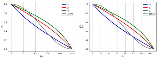 Figure 1. Comparison of new step sizes and cosine step size.
 - We demonstrate that the proposed step sizes achieve an convergence rate for smooth non-convex functions.
- We analyze the convergence behavior of SGD applied to non-smooth and non-convex functions, utilizing new step sizes. Theoretical guarantees for the convergence are provided, supporting the effectiveness of the new step sizes.
- We conduct extensive experiments on popular datasets, showing that the proposed step sizes outperform the cosine step size and achieve superior results compared to other existing step sizes.
This paper is organized in the following manner: Section 1 details the newly developed trigonometric step sizes and explores their characteristics. The convergence rates of these step sizes, particularly for smooth non-convex functions, are analyzed in Section 2. Section 3 analyzes the convergence of SGD for non-smooth and non-convex functions based on the new trigonometric step sizes. Numerical results derived from the application of these novel step sizes are presented and examined in Section 4. The paper concludes with Section 5, where we encapsulate our key discoveries and provide conclusions from our research.
In this paper, we use the following notations:
- We represent the Euclidean norm of any vector using .
- The terms and denote the nonnegative orthant and positive orthant of , respectively.
- and are used to represent the optimal point and the optimal value of the objective function.
- The expression signifies that for some positive constant , the relationship holds true for all .
2. Formulation of the Problem and Proposed Methodology
We focus on the following optimization problem:
where represents the loss function associated with the i-th training sample, and is the variable to be optimized. The scalar n denotes the total number of training samples. This minimization problem is foundational in machine learning, particularly in the training of models where the objective is to minimize the average loss across all samples. Various iterative methods have been developed to solve Equation (1) efficiently, especially when the dimensionality d or the number of samples n is large [28]. Among these methods, SGD is particularly favored for its efficiency in high-dimensional settings and its ability to handle large-scale data [17,29].
SGD updates the variable x by selecting a random training sample at each iteration k and applying the update rule:
where is the step size at iteration k, and is the gradient of the loss function with respect to the variable at the current iteration [30]. This approach enables SGD to make incremental adjustments to x, gradually converging to a minimum of the objective function.
Our analysis and results in this paper are based on the following key assumptions:
Assumption 1.
The function f is differentiable and L-smooth, meaning that for all , there exists a constant such that
This assumption ensures that the gradients do not change too rapidly, which is crucial for the stability and convergence of the SGD algorithm.
Assumption 2.
For any random , the variance of the stochastic gradient is bounded, such that
This assumption controls the noise in the gradient estimates, which is a critical factor in the convergence behavior of SGD.
Assumption 3.
The objective function f is bounded below on , ensuring that there exists a lower bound such that for all . Moreover, the function f is upper bounded by if for any , we have
This assumption guarantees that the optimization problem is well posed, preventing the algorithm from diverging as it iterates.
These assumptions form the foundation for the theoretical analysis of the convergence properties of SGD and guide the development of effective step size strategies.
2.1. New Step Sizes
In their groundbreaking work, Ref. [8] introduced the cosine step size, which is defined as follows:
where is the initial learning rate. This step size has demonstrated strong performance compared to other step sizes, primarily because it does not rapidly converge to zero, thereby allowing SGD to maintain better performance over time. However, one limitation of the cosine step size is its suboptimal behavior concerning the probability distribution . This issue inspired us to develop new step sizes that offer two key advantages:
- They do not converge to zero rapidly, ensuring sustained learning throughout the iterations.
- They exhibit a more desirable probability distribution, allocating smaller values during the initial iterations and larger values towards the final iterations compared to the cosine step size.
Based on these objectives, we propose three novel trigonometric step sizes for the SGD method:
All of these new step sizes begin at , and and converge to zero by the final iteration T.
Figure 1 illustrates the behavior of the proposed step sizes compared to the cosine step size. The figure reveals that the new step sizes do not rapidly approach zero; instead, they retain higher values, particularly in the final iterations, which enhances the algorithm’s performance even at later stages. Furthermore, the figure on the right highlights the probability distribution for the new step sizes in comparison to the cosine step size. It is evident that and allocate smaller values during the initial iterations and larger values towards the final iterations, providing the algorithm with a better chance of selecting and utilizing the final iterations effectively.
2.2. Algorithm
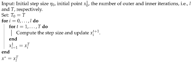
Here, we apply the warm restart SGD algorithm introduced by Loshchilov and Hutter in [8]. The algorithm involves an outer loop and an inner loop. The outer loop periodically resets the learning rate back to its initial value, usually coinciding with the completion of a training cycle or epoch. This reset mechanism is intended to prevent the model from converging prematurely into local minima, promoting a broader exploration of the solution space by reintroducing larger learning rates at specific intervals. The inner loop follows the conventional SGD approach, where model parameters are updated based on the gradients calculated from a randomly selected subset of the training data. During this phase, the learning rate gradually decreases according to the new trigonometric step sizes, eventually reaching a minimum by the end of the cycle. Once this minimum is achieved, the outer loop activates the warm restart, resetting the learning rate and beginning a new cycle. This entire process is outlined in Algorithm 1, where T denotes the number of iterations within the inner loop, and l indicates the total number of epochs for the algorithm.
| Algorithm 1 SGD with Warm Restarts New Step Sizes |
 |
3. Convergence Results
To establish the convergence rate, we first present several fundamental lemmas that are crucial for deriving the convergence results. The following lemma offers the necessary bounds on the function, which are critical for analyzing the behavior of the trigonometric step sizes and proving the overall convergence of the algorithm.
Lemma 1.
For all , the following inequalities are valid:
- 1.
- 2.
Proof.
To prove the first inequality, consider the function and examine its derivative. Specifically, we find that , where . The derivative of is for all . Since is a decreasing function with , it follows that on this interval. Therefore, , which implies that is a decreasing function on . As a result, we obtain the following:
The proof of the second inequality follows directly and is omitted here for brevity. □
Lemma 2.
For the function , we have
Proof.
We have
where the first inequality is derived from the fact that for all x. The second inequality follows from Lemma 1. Finally, the last equality is obtained by recognizing that . □
Lemma 3.
For the function , we have
Proof.
We have
□
Now, we present the upper and lower bounds for the second step size, denoted as .
Lemma 4.
For the step size , we have
Proof.
We have
where the last inequality is obtained using this fact that . □
Lemma 5.
For any , we have the following:
Lemma 6.
For the step size , we have
Proof.
Using Lemma 5, we have
On the other hand, we can show that
Therefore, we have
□
Lemma 7.
For the step size , we have
Proof.
We have
where the last inequality is obtained using this fact that . □
Lemma 8.
For the step size , we have
Proof.
Using Lemma 5, we have
□
To achieve the convergence rate, we recall Lemma 7 in [16].
Lemma 9
(Lemma 7.1 in [16]). Assuming that f is an L-smooth function and Assumption 2 is satisfied, if , then SGD guarantees the following results:
The next theorem establishes a convergence rate of for SGD based on the step size for smooth non-convex functions. Similar results can also be obtained for two other step sizes, and as such, we omit their proofs here.
Theorem 1.
Under Assumptions 1 and 2, the SGD algorithm with the new step size guarantees
where is a random iterate drawn from the sequence with corresponding probabilities . The probabilities are defined as .
Proof.
Using the fact that is randomly selected from the sequence with probability and Jensen’s inequality, we have
We obtain the first and second inequalities by applying Jensen’s inequality and utilizing Lemma 9. Furthermore, considering the fact that and Lemmas 2 and 3, we obtain the following:
Now, using the definition , we have
Setting , we can conclude that
□
Remark 1.
The conditions outlined in the theorem are satisfied for the new step sizes. In fact, Assumption 1, which mandates that the objective function f be differentiable and L-smooth, is fulfilled by the tan step size, ensuring that the gradient variations remain controlled. Assumption 2, which asserts that the variance of the stochastic gradient is bounded, holds true as the tan step size does not violate the bounded variance condition. The step size exhibits a monotonically decreasing behavior, consistent with the requirements for SGD convergence. Additionally, the probabilities , as defined in the theorem, align with the decreasing nature of the tan step size.
4. Convergence Analysis for Non-Smooth Optimization
In this section, we focus on the optimization problem where the objective function is non-smooth and non-convex, presenting additional challenges for convergence analysis. We investigate the convergence behavior of the SGD when applied to such functions, utilizing newly proposed step sizes that facilitate progress toward the global minimum. Our proof is based on the subgradient approach, which is well suited for handling non-smooth functions. Theoretical guarantees for the convergence of the algorithm under some common conditions are also provided. To address this, consider the following optimization problem:
Here, represents the global minimum of the objective function f, which is commonly referred to as the loss function in machine learning contexts. The vector x is the optimization variable, typically representing a set of weights in a model.
For the optimization problem (5), we adopt the following assumptions:
- A vector g is considered a subgradient of at x if it satisfies the inequality
- The subgradient method updates the optimization variable x using the function value and a subgradient g from the subdifferential set . The iterative update rule is given by the following:where is the step size at iteration t. This approach allows optimization over non-smooth functions by following a descent direction within the subdifferential set.
Additionally, by utilizing the properties of the newly proposed step sizes, as outlined in Lemma 2, and for sufficiently large T, we can derive the following results:
The following theorem presents the convergence results of SGD for non-smooth, non-convex functions when the newly proposed step sizes are applied. The proof is inspired by the work of [31].
Theorem 2.
Proof.
which, combined with the assumption in (11), leads to
Multiplying both sides of (13) by , we obtain
Substituting this into the recursive update equation for the iterates, we have
Since for some constant [32], this leads to
By applying this recursively and using the step size condition (8), we obtain
Finally, since as , the right-hand side of (15) tends to 0, leading to a contradiction. This completes the proof of the theorem, showing that as . □
To prove the theorem, we aim to show that for every , there exists an index such that for all , the inequality
holds. We proceed by contradiction. Assume there exists a constant such that for every , we have
where denotes a subsequence of .
- By applying the subgradient condition (6) with and , we obtain
5. Numerical Results
In this section, we present the evaluation results of our proposed schemes on the CIFAR-10, CIFAR-100, and FashionMNIST datasets. These are popular datasets used in machine learning, particularly for image classification tasks. To evaluate the performance of our proposed methods, we conducted experimental studies comparing them with state-of-the-art techniques. These comparisons provide valuable insights into the effectiveness of our approach and its relative standing against existing methods. The performance is measured using accuracy on the test sets, and we compare our methods against several baseline models. Now, let us explore the specific strategies, datasets, and learning models used for the classification task in more detail. The implementation was carried out using Python 3.9 with PyTorch 2.6.0 as the deep learning framework. The training was performed on a laptop equipped with an Intel Core i9-13000 processor, 16 GB of RAM, and an NVIDIA 4050 GPU.
5.1. Datasets
CIFAR-10, CIFAR-100, and FashionMNIST are widely used benchmark datasets in machine learning and computer vision. CIFAR-10 consists of 60,000 color images divided into 10 classes, each containing 6000 images, such as airplanes, cars, and birds, making it a popular choice for evaluating image classification algorithms. CIFAR-100 is a more challenging variant that contains 100 classes with 600 images per class, providing a finer granularity of categories, which tests the robustness and versatility of models. On the other hand, FashionMNIST is a dataset of 70,000 grayscale images representing various clothing items, such as shirts, shoes, and bags, serving as a more challenging alternative to the traditional MNIST dataset of handwritten digits. Together, these datasets provide a comprehensive evaluation framework for assessing the performance of image classification algorithms across different complexities and domains.
5.2. Models
For the classification task on the FashionMNIST dataset, we utilized a Convolutional Neural Network (CNN) model. Here is a breakdown of the CNN architecture we implemented. It features two convolutional layers, each using a filter size of . We applied padding of 2 to ensure that the output feature maps maintain the same spatial dimensions as the input. Additionally, the model includes two max-pooling layers with a kernel size of . Max-pooling helps reduce spatial dimensions while retaining important features and eliminating irrelevant details. To further process the extracted features, the model has two fully connected layers, each consisting of 1024 hidden nodes. The activation function employed for these hidden nodes is the Rectified Linear Unit (ReLU), which introduces non-linearity and enables the model to effectively learn complex patterns.
To assess the effectiveness of the algorithms on the CIFAR10 dataset, we utilized a deep learning framework called the 20-layer Residual Neural Network (ResNet). Introduced by [33], ResNet has demonstrated significant success in a range of computer vision applications. The model employs cross-entropy loss as its loss function.
In the case of the CIFAR100 dataset, the deep learning model employed is a DenseNet-BC model that consists of 100 layers, with a growth rate of 12 [34]. The overall architecture of this dense model is depicted in Figure 2.
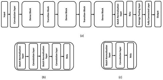
Figure 2.
(a) Overall structure of DenseNet-BC model: (b) dense block; (c) transition block.
5.3. Algorithm and Set Up
In this section, we perform an extensive comparative analysis to assess different step sizes. We take into account the following step sizes:
We investigate a range of step size update strategies, including SGD with constant step size, step sizes that decay at rates of and , cosine step size updates, and newly introduced step decay methods labeled as Alpha (), Beta (), and Gamma (), respectively. In this context, t represents the iteration number within the inner loop, where each outer iteration comprises multiple mini-batch training iterations.
Additionally, we evaluate the effectiveness of the newly introduced step decay methods in comparison to Adam [3], the SGD+Armijo method [30], PyTorch’s ReduceLROnPlateau scheduler (referred to as ReduceLROnPlateau), and a stagewise step size strategy. In this analysis, we designate the points where the step size is reduced in the stagewise approach as milestones. It is worth mentioning that since Nesterov momentum is utilized across all SGD variants, the stagewise step decay method effectively captures the performance of multistage accelerated algorithms (e.g., [35]). To optimize the hyperparameters of the proposed step decay method across the three datasets, we employed a two-stage grid search using the validation set. In the first stage, we performed a coarse grid search to identify a set of candidate hyperparameters that yielded the best validation performance. Based on these initial results, we conducted a second, more fine-grained search around the most promising values to determine the optimal hyperparameter configuration. For the initial step size, the first-stage grid search was conducted over the range {0.00001, 0.0001, 0.001, 0.01, 0.1, 0.2, 0.3, 0.4, 0.5, 0.6, 0.7, 0.8, 0.9, 1}. For CIFAR-10 and CIFAR-100, the second-stage refinement focused on the range {0.11, 0.12, 0.13, 0.14, 0.15, 0.16, 0.17, 0.18, 0.19, 0.20, 0.21, 0.22, 0.23, 0.24, 0.25}. The optimal initial step sizes were found to be 0.2 for CIFAR-10 and 0.15 for CIFAR-100. For FashionMNIST, the best initial step sizes were 0.01 for the Alpha step size and 0.02 for both the Beta and Gamma step sizes. For other step size strategies, we adopted the hyperparameters reported in [9]. We summarize the hyperparameter values for the aforementioned methods in Table 1. Moreover, the symbol − indicates that the respective step size does not require or utilize the specified parameter.

Table 1.
The hyperparameter values for the methods employed on the FashionMnist, CIFAR10, and CIFAR100 datasets. The parameter for the Alpha, Beta, and Gamma methods is consistent with , , and , respectively.
5.4. Results
We conducted three series of experiments to compare the aforementioned methods across various aspects, as detailed below:
- Figure 3 presents the outcomes of implementing our new step decay methods. In experiments conducted on the FashionMNIST dataset, the proposed Beta decay step size demonstrates superior performance in terms of training loss compared to the other methods. However, the efficiency of all proposed decay step sizes—Alpha, Beta, and Gamma—remains largely comparable when evaluated based on test accuracy. For the CIFAR10 and CIFAR100 datasets, the Alpha decay step size shows better performance in training loss, while both Beta and Gamma exhibit superior results in terms of test accuracy.
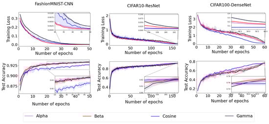 Figure 3. Comparison of tan and cosine step sizes.
 - The proposed decay step sizes were inspired by cosine step decay and designed to address its limitations, as discussed in Section 2.1. To evaluate their effectiveness, we conducted a series of experiments focusing on training loss and test accuracy. The results, presented in Figure 3, indicate that the proposed decay step sizes outperform cosine step decay in both training loss and test accuracy.
- To improve the clarity of our results, we have organized the methods into two separate categories, as shown in Figure 4 and Figure 5. In our experiments with the FashionMnist dataset, both the established methods SGD+Armijo and stagewise step decay-1 milestones successfully reduced training loss to nearly zero; however, our proposed Gamma decay step size outperformed all other approaches in terms of test accuracy. Similarly, for the CIFAR10 dataset, the proposed step sizes exhibited better performance than competing methods in both training loss and test accuracy. In the CIFAR100 dataset, although the established SGD+Armijo and ReduceLROnPlateau methods also achieved training loss close to zero, our proposed decay step sizes excelled compared to other techniques regarding test accuracy.
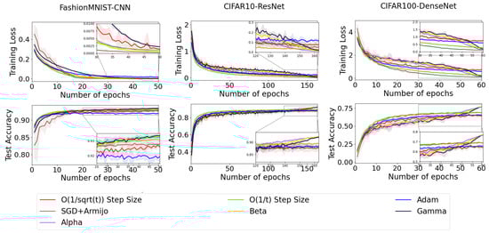 Figure 4. Comparison of new proposed step size and four other step sizes.
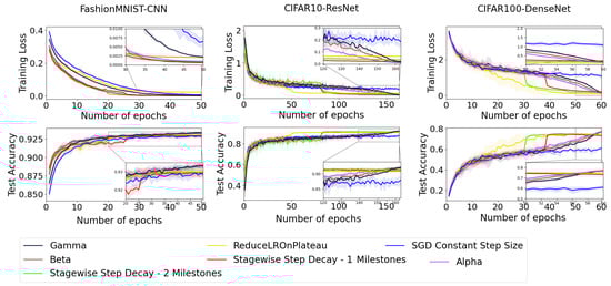 Figure 5. Comparison of new proposed step size and four other step sizes.
 - The average training loss and test accuracy for the FashionMNIST, CIFAR10, and CIFAR100 datasets, based on five runs with different random seeds, are presented in Table 2, Table 3 and Table 4. The bolded values in Table 2, Table 3 and Table 4 represent the highest accuracy achieved and lowest training loss for each dataset among all different step sizes. Analyzing the data from these tables leads us to the following observations:
Table 2. Average final training loss and test accuracy on the FashionMNIST dataset. The confidence intervals of the mean loss and accuracy value over 5 runs starting from different random seeds.
Table 3. Average final training loss and test accuracy obtained by 5 runs starting from different random seeds and ± is followed by an estimated margin of error under confidence on the CIFR10 dataset.
Table 4. Average final training loss and test accuracy obtained by 5 runs starting from different random seeds and ± is followed by an estimated margin of error under confidence on the CIFR100 dataset using the DenseNet-BC model.
- −
- In the case of the FashionMNIST dataset (refer to Table 2), while the SGD+Armijo step size yielded the lowest training loss, the proposed Gamma step size achieved the highest test accuracy.
- −
- For the CIFAR10 dataset (as shown in Table 3), the Alpha step size resulted in the best training loss, whereas the Beta step size produced the highest test accuracy.
- −
- Regarding the CIFAR100 dataset (illustrated in Table 4), while the Cosine step size yielded the lowest training loss, the proposed Beta step size achieved the highest test accuracy.
Table 5 presents a comparative analysis of the three new step size strategies and the cosine step size across three datasets, i.e., FashionMNIST, CIFAR10, and CIFAR100. While all methods achieve near-perfect training performance, their effectiveness varies in test performance, highlighting differences in generalization capability. For FashionMNIST and CIFAR10, the Alpha step size consistently achieves the highest test precision, recall, and F1-score, suggesting superior generalization compared to other approaches. Conversely, the cosine step size exhibits the lowest test performance across all datasets, indicating that its step size schedule may be suboptimal for maintaining generalization. In the more complex CIFAR100 dataset, Gamma outperforms all other methods in test performance, achieving the highest precision, recall, and F1-score. This suggests that Gamma’s step size adaptation may better suit high-dimensional classification tasks, where effective learning dynamics are crucial.
Table 5.
Performance comparison of different step size methods (Cosine, Alpha, Beta, and Gamma) on the FashionMNIST, CIFAR10, and CIFAR100 datasets, showing final training and test precision, recall, and F1 scores.
Figure 6 presents the confusion matrix for the Alpha method evaluated on the test set, providing insights into the model’s performance on both the FashionMNIST and CIFAR-10 datasets. For the FashionMNIST dataset, the matrix highlights the accuracy of the model in classifying 10 different clothing categories, revealing the distribution of correctly and incorrectly predicted labels. For the CIFAR-10 dataset, which consists of 10 diverse classes such as cars, airplanes, and animals, the confusion matrix helps assess the model’s ability to distinguish between more complex visual features.
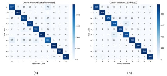
Figure 6.
Confusion matrix of the Alpha method evaluated on the test set for (a) the FashionMNIST dataset and (b) the CIFAR-10 dataset.
6. Conclusions and Future Work
This paper introduced a novel set of trigonometric step sizes based on tangent functions, which were integrated into the warm restart Stochastic Gradient Descent (SGD) framework. It was demonstrated that the proposed step sizes achieved an convergence rate for smooth non-convex functions, aligning with theoretical expectations. Furthermore, the analysis was extended to non-smooth and non-convex optimization landscapes, where standard convergence guarantees were more challenging. To validate the effectiveness of the proposed approach, extensive experiments were conducted using the FashionMNIST, CIFAR-10, and CIFAR-100 datasets. The performance of the proposed step sizes was benchmarked against nine widely used step size strategies, including the cosine step size. Empirical results indicated that the method consistently outperformed existing approaches in terms of both classification accuracy and loss reduction.
Future research should focus on extending the proposed trigonometric step sizes to a broader range of optimization problems. One promising direction is the investigation of their effectiveness in strongly convex and convex non-smooth functions, where theoretical convergence guarantees could provide deeper insights into their stability and efficiency. Moreover, analyzing the impact of these step sizes on saddle point avoidance and escaping sharp minima would further enhance their applicability. Additionally, exploring their integration into adaptive learning rate strategies, such as the Armijo line search method, could offer practical benefits in large-scale deep learning applications. Further empirical studies could be conducted on various neural network architectures, including transformer-based models and generative adversarial networks, to assess their generalization capabilities compared to alternative step size schedules.
Author Contributions
Conceptualization, S.F.H.; methodology, S.F.H. and M.S.S.; visualization, M.S.S.; investigation, S.F.H. and M.S.S.; writing—original draft preparation, S.F.H. and M.S.S.; writing—review and editing, S.F.H. and M.S.S. All authors have read and agreed to the published version of the manuscript.
Funding
This research received no external funding.
Data Availability Statement
The datasets used in this paper are available from the following link: https://www.cs.toronto.edu/~kriz/cifar.html, accessed on 15 March 2024.
Acknowledgments
The authors would like to thank the editors and anonymous reviewers for their constructive comments.
Conflicts of Interest
The authors declare no conflicts of interest.
Abbreviations
The following abbreviations are used in this manuscript:
| SGD | Stochastic Gradient Descent |
| SGDR | Stochastic Gradient Descent with Warm Restarts |
| CNN | Convolutional Neural Network |
| ResNet | Residual Neural Network |
| RNN | Recurrent Neural Networks |
References
- Bottou, L. Large-scale machine learning with stochastic gradient descent. In Proceedings of the COMPSTAT’2010: 19th International Conference on Computational Statistics, Paris, France, 22–27 August 2010; Keynote, Invited and Contributed Papers. Springer: Berlin/Heidelberg, Germany; pp. 177–186. [Google Scholar]
- Goodfellow, I.; Bengio, Y.; Courville, A. Deep Learning; Adaptive Computation and Machine Learning Series; MIT Press: Cambridge, MA, USA, 2016; Volume 1. [Google Scholar]
- Diederik, P.K. Adam: A method for stochastic optimization. arXiv 2014, arXiv:1412.6980. [Google Scholar]
- Ruder, S. An overview of gradient descent optimization algorithms. arXiv 2016, arXiv:1609.04747. [Google Scholar]
- Sutskever, I.; Martens, J.; Dahl, G.; Hinton, G. On the importance of initialization and momentum in deep learning. In Proceedings of the International Conference on Machine Learning, Atlanta, GA, USA, 17–19 June 2013; pp. 1139–1147. [Google Scholar]
- Smith, L.N. Cyclical learning rates for training neural networks. In Proceedings of the 2017 IEEE Winter Conference on Applications of Computer Vision (WACV), Santa Rosa, CA, USA, 24–31 March 2017; pp. 464–472. [Google Scholar]
- Zeiler, M. Adadelta: An adaptive learning rate method. arXiv 2012, arXiv:1212.5701. [Google Scholar]
- Loshchilov, I.; Hutter, F. SGDR: Stochastic gradient descent with warm restarts. arXiv 2016, arXiv:1608.03983. [Google Scholar]
- Li, X.; Zhuang, Z.; Orabona, F. A second look at exponential and cosine step sizes: Simplicity, adaptivity, and performance. In Proceedings of the International Conference on Machine Learning, Virtual, 18–24 July 2021; pp. 6553–6564. [Google Scholar]
- Vrbanič, G.; Podgorelec, V. Efficient ensemble for image-based identification of pneumonia utilizing deep CNN and SGD with warm restarts. Expert Syst. Appl. 2022, 187, 115834. [Google Scholar] [CrossRef]
- Liu, Z. Super Convergence Cosine Annealing with Warm-Up Learning Rate. In Proceedings of the CAIBDA 2022; 2nd International Conference on Artificial Intelligence, Big Data and Algorithms, Nanjing, China, 17–19 June 2022; pp. 1–7. [Google Scholar]
- Li, F.; Li, Y.; Sun, B.; Cui, H.; Yan, J.; Feng, P.; Peng, X. A Novel DenseNet with Warm Restarts for Gas Recognition in Complex Airflow Environments. Microchem. J. 2024, 197, 109864. [Google Scholar] [CrossRef]
- Shamaee, M.S.; Hafshejani, S.F. A Novel Sine Step Size for Warm-Restart Stochastic Gradient Descent. Axioms 2024, 13, 857. [Google Scholar] [CrossRef]
- Shamaee, M.S.; Hafshejani, S.F.; Saeidian, Z. New logarithmic step size for stochastic gradient descent. Front. Comput. Sci. 2025, 19, 191301. [Google Scholar] [CrossRef]
- Mishra, P.; Sarawadekar, K. Polynomial Learning Rate Policy with Warm Restart for Deep Neural Network. In Proceedings of the TENCON 2019-2019 IEEE Region 10 Conference (TENCON), Kochi, India, 17–20 October 2019; pp. 2087–2092. [Google Scholar]
- Wang, X.; Magnússon, S.; Johansson, M. On the convergence of step decay step-size for stochastic optimization. Adv. Neural Inf. Process. Syst. 2021, 34, 14226–14238. [Google Scholar]
- Nemirovski, A.; Juditsky, A.; Lan, G.; Shapiro, A. Robust stochastic approximation approach to stochastic programming. SIAM J. Optim. 2009, 19, 1574–1609. [Google Scholar] [CrossRef]
- Ghadimi, S.; Lan, G. Stochastic first-and zeroth-order methods for nonconvex stochastic programming. SIAM J. Optim. 2013, 23, 2341–2368. [Google Scholar] [CrossRef]
- Moulines, E.; Bach, F. Non-asymptotic analysis of stochastic approximation algorithms for machine learning. Adv. Neural Inf. Process. Syst. 2011, 24, 451–459. [Google Scholar]
- Rakhlin, A.; Shamir, O.; Sridharan, K. Making gradient descent optimal for strongly convex stochastic optimization. arXiv 2011, arXiv:1109.5647. [Google Scholar]
- Ge, R.; Kakade, S.M.; Kidambi, R.; Netrapalli, P. The step decay schedule: A near optimal, geometrically decaying learning rate procedure for least squares. Adv. Neural Inf. Process. Syst. 2019, 32, 14977–14988. [Google Scholar]
- Nesterov, Y. Smooth minimization of non-smooth functions. Math. Program. 2005, 103, 127–152. [Google Scholar] [CrossRef]
- Tibshirani, R. Regression Shrinkage and Selection via the Lasso. J. R. Stat. Soc. Ser. B 1996, 58, 267–288. [Google Scholar] [CrossRef]
- Glorot, X.; Bordes, A.; Bengio, Y. Deep Sparse Rectifier Neural Networks. In Proceedings of the 14th International Conference on Artificial Intelligence and Statistics (AISTATS), Fort Lauderdale, FL, USA, 11–13 April 2011; pp. 315–323. [Google Scholar]
- Shor, N.Z. Minimization Methods for Non-Differentiable Functions; Springer: Berlin/Heidelberg, Germany, 2012. [Google Scholar]
- Beck, A.; Teboulle, M. A Fast Iterative Shrinkage-Thresholding Algorithm for Linear Inverse Problems. SIAM J. Imaging Sci. 2009, 2, 183–202. [Google Scholar] [CrossRef]
- Nesterov, Y. A Method of Solving the Convex Programming Problem with Convergence Rate O(1/k2). Dokl. Akad. Nauk. SSSR 1983, 269, 543–547. [Google Scholar]
- Nocedal, J.; Wright, S.J. Numerical Optimization; Springer Series in Operations Research and Financial Engineering; Springer: New York, NY, USA, 1999. [Google Scholar]
- Robbins, H.; Monro, S. A stochastic approximation method. Ann. Math. Stat. 1951, 22, 400–407. [Google Scholar] [CrossRef]
- Vaswani, S.; Mishkin, A.; Laradji, I.; Schmidt, M.; Gidel, G.; Lacoste-Julien, S. Painless stochastic gradient: Interpolation, line-search, and convergence rates. Adv. Neural Inf. Process. Syst. 2019, 32, 3732–3745. [Google Scholar]
- El Mouatasim, A.; de Cursi, J.E.S.; Ellaia, R. Stochastic perturbation of subgradient algorithm for nonconvex deep neural networks. Comput. Appl. Math. 2023, 42, 167. [Google Scholar] [CrossRef]
- Dem’vanov, V.F.; Vasil’ev, L.V. Nondifferentiable Optimization; Optimization Software, Inc. Publications Division; Springer: New York, NY, USA, 1985. [Google Scholar]
- He, K.; Zhang, X.; Ren, S.; Sun, J. Deep residual learning for image recognition. In Proceedings of the IEEE Conference on Computer Vision and Pattern Recognition, Las Vegas, NV, USA, 27–30 June 2016; pp. 770–778. [Google Scholar]
- Huang, G.; Liu, Z.; Van Der Maaten, L.; Weinberger, K.Q. Densely connected convolutional networks. In Proceedings of the IEEE Conference on Computer Vision and Pattern Recognition, Honolulu, HI, USA, 21–26 July 2017; pp. 4700–4708. [Google Scholar]
- Aybat, N.S.; Fallah, A.; Gurbuzbalaban, M.; Ozdaglar, A. A universally optimal multistage accelerated stochastic gradient method. Adv. Neural Inf. Process. Syst. 2019, 32, 8525–8536. [Google Scholar]
Disclaimer/Publisher’s Note: The statements, opinions and data contained in all publications are solely those of the individual author(s) and contributor(s) and not of MDPI and/or the editor(s). MDPI and/or the editor(s) disclaim responsibility for any injury to people or property resulting from any ideas, methods, instructions or products referred to in the content. |
© 2025 by the authors. Licensee MDPI, Basel, Switzerland. This article is an open access article distributed under the terms and conditions of the Creative Commons Attribution (CC BY) license (https://creativecommons.org/licenses/by/4.0/).