Article

Enhancing Unmanned Aerial Vehicle Object Detection via Tensor Decompositions and Positive–Negative Momentum Optimizers

1
Department of Mathematical Modelling, North-Caucasus Federal University, 355009 Stavropol, Russia
2
Computer-Aided Design Department, St. Petersburg Electrotechnical University “LETI”, 5 Professora Popova St., 197022 Saint Petersburg, Russia
*
Authors to whom correspondence should be addressed.
Mathematics 2025, 13(5), 828; https://doi.org/10.3390/math13050828
Submission received: 16 January 2025 / Revised: 21 February 2025 / Accepted: 28 February 2025 / Published: 1 March 2025

Abstract

:
The current development of machine learning has advanced many fields in applied sciences and industry, including remote sensing. In this area, deep neural networks are used to solve routine object detection problems, satisfying the required rules and conditions. However, the growing number and difficulty of such problems cause the developers to construct machine learning models with higher computational complexities, such as an increased number of hidden layers, epochs, learning rate, and rate decay. In this paper, we propose the Yolov8 architecture with decomposed layers via canonical polyadic and Tucker methods for accelerating the solving of the object detection problem in satellite images. Our positive–negative momentum approaches enabled a reduction in the loss in precision and recall assessments for the proposed neural network. The convolutional layer factorization reduces the shapes and accelerates the computations at kernel nodes in the proposed deep learning models. The advanced optimization algorithms achieve the global minimum of loss functions, which makes the precision and recall metrics superior to the ones for their known counterparts. We examined the proposed Yolov8 with decomposed layers, comparing it with the conventional Yolov8 on the DIOR and VisDrone 2020 datasets containing the UAV images. We verified the performance of the proposed and known neural networks on different optimizers. It is shown that the proposed neural network accelerates the solving object detection problem by 44–52%. The proposed Yolov8 with Tucker and canonical polyadic decompositions has greater precision and recall metrics than the usual Yolov8 with known analogs by 0.84–0.94 and 0.228–1.107 percentage points, respectively.

1. Introduction

One of the key problems in remote sensing, computer vision, and artificial intelligence is object detection in images. This problem arises in various scientific, health, and industrial areas, affecting the quality of modern intellectual systems. Since the 1990s, many researchers have been developing methods for solving the object detection problem. Avionics, radar, space radio, and telescope systems utilize expert system models to increase the accuracy of feature detection by researchers. Nowadays, the rapid development of UAV systems equipped with cameras requires more advanced technologies for object detection on Earth. Instead of expert systems, researchers and engineers prefer to utilize deep learning models. This technique can be found in various areas of human activity, such as remote sensing [1], geolocation [2], astronomy [3], and others.
Due to the development of deep neural networks, valuable gains can be made when using the features of convolutional neural networks (R-CNN) [4]. Such machine learning models contain multiple convolution, pooling, and full-dense layers. The convolution operation analyzes the patterns in the image by compressing it to digital data, which the multilayer perceptron block processes and transfers to backpropagation. Next, the loss function determines the distinction between the true and obtained results. Finally, the backpropagation algorithm updates the weight values in the convolutional and linear layers via gradient-based optimization algorithms. The expressivity and robustness of self-learning algorithms allow us to learn informative object representations without the need to design features manually. The R-CNN improved the quality of solving the object detection problem in images of arbitrary datasets. Since 2014, there have been many promising neural network architectures that detect objects in images relatively fast and with the required precision. Scholars often utilize the fast R-CNN for small object detection in optical remote sensing images. For example, the authors of [5] used SPP-Net to detect the object in speckle noise conditions. Multi-scale object detection in remote sensing imagery was solved using the FRCN model. However, one of the best models that solve the object detection problem is You Only Look Once (Yolov8) neural network [6]. The Yolov8 architecture proved its stability and performance in object detection in images and videos. Moreover, this model is suitable for working with data that have been noised.

1.1. Motivation

Modern neural network architectures that solve the object detection problem [7] with the required precision consume too much computational time and hardware resources. For the acceleration of neural network training, many researchers perform dataset configuration [8], such as compressing [9] and reducing [10]. To reduce the training time of deep neural networks, the authors of paper [11] made the computations using the Strassen and Strassen–Winograd matrix multiplication algorithm, thus obtaining higher performance and preserving precision. These methods made computation in convolutional layers faster. However, such an approach consumes even more hardware resources. In one study [12], the authors use the Ozaki matrix multiplication method in convolutional layers. This approach reduces the computational and time costs. However, it cannot maintain the required precision. Therefore, one needs an approach that may accelerate deep neural network training while maintaining accuracy. One of the most suitable techniques is convolutional layer conversion by tensor decomposition. The idea of tensor-based neural networks [13] came from quantum computing, where the operation over wave functions is similar to analogs, which can be found in tensor analysis. In [14], the authors achieved a higher training speed of neural networks with a minimal loss of accuracy using tensor decompositions. The most utilized tensor decompositions are canonical polyadic (CP) and Tucker. Such approaches consider the convolutional layer as a three-order tensor and decompose it into a sublayer with smaller shapes. It reduces the computational costs and time consumption. However, it remains difficult to maintain the required precision and recall metrics. This problem can be solved by using advanced loss function optimization algorithms. The state-of-the-art (SOTA) stochastic gradient descent (SGD) and adaptive moment estimation (Adam) can achieve the required precision in the case of CP and Tucker decompositions. SGD finds the minimum, considering the gradient directions. Adam uses the exponential moving averages of the gradient and its square. These techniques do not necessarily attain the global minimum of loss function because they do not distinguish the local and global extremes. For example, such flaws can be observed in the minimization of Rastrigin and Rosenbrock test functions. Therefore, one needs to use the optimizer, which can converge to a global minimum for a lesser number of epochs. In papers [15,16], we developed positive–negative momentum approaches such as DiffPNM, YogiPNM, and PNMBeleif. DIffPNM let the ensemble learning model solve the pattern recognition problem in satellite images from the UC-Merced dataset. YogiPNM and PNMBelief allowed the multi-modal neural network to solve the skin lesion recognition problem better than existing analogs. In this work, we propose the Yolov8 architectures with the convolutional decomposition by CP-Astrid and Tucker-2 models and train them using DiffPNM, YogiPNM, and PNMBelief. We clearly demonstrate that the usual Yolov8 with SGD and Adam is inferior in precision and recall properties to accelerated Yolov8 with positive–negative momentum approaches.

1.2. Our Contribution

The main contributions of our study can be summarized as follows:
(i) New Yolov8-CP-Astrid and Yolov8-Tucker-2 neural networks are proposed. Such models can train faster because of the decomposed convolutional layers.
(ii) We integrated our optimization methods DiffPNM, YogiPNM, and PNMBelief into the proposed Yolov8-CP-Astrid and Yolov8-Tucker-2 neural networks. This technique allowed us to minimize the precision and recall losses.
(iii) In the experimental part of the study, we applied the proposed Yolov8-CP-Astrid and Yolov8-Tucker-2 to solve the object detection problem on the DIOR dataset. Our models achieved greater precision and recall metrics than conventional Yolov8 models with SGD and Adam by 0.84–0.94 and 0.228–10.107 percentage points, correspondingly, and reduce the training time by 44–52%.
Thus, the proposed Yolov8-CP-Astrid and Yolov8-Tucker-2 neural networks allowed to improve the accuracy and rate of solving the object detection problem on the DIOR dataset. It should be noted that any deep neural network can be decomposed in several tensor decomposition models. The application of advanced optimization algorithms can minimize precision and recall losses.
The rest of the paper is organized as follows. In Section 2, Yolov8 architecture, tensor decompositions, and optimization methods are described. In Section 3, we propose the Yolov8-CP-Astrid and Yolov8-Tucker-2 neural networks. In Section 4, we demonstrate the results of solving the object detection problem in images from the DIOR dataset using known and proposed neural network architectures. Section 5 discusses the further improvements and applications of the proposed Yolov8-CP-Astrid and Yolov8-Tucker-2 neural networks. Finally, in Section 6, some conclusions on the obtained results of solving the object detection problem via the proposed Yolov8-CP-Astrid and Yolov8-Tucker-2 neural networks are given.

2. State of the Art

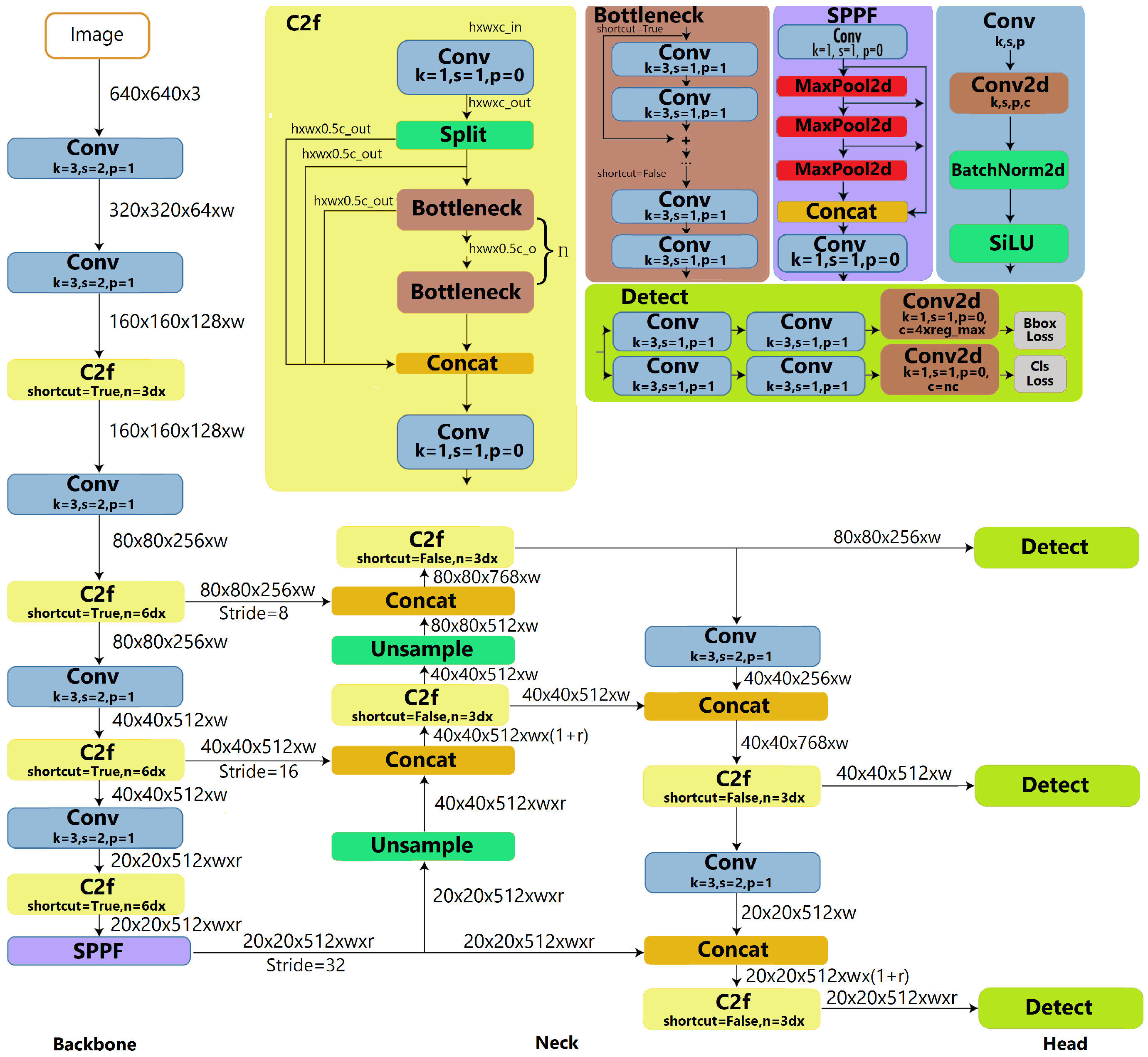
2.1. Yolov8 Architecture

The main feature of Yolo-based neural network architectures is the sequential utilization of special blocks: backbone, neck, and head. The backbone block is the core part of the YOLOv8. It extracts features from the input RGB color images. The neck block aggregates and processes the features of different scales extracted by the backbone network. This block embraces a feature pyramid network structure [6], which effectively fuses features of various scales to construct a more comprehensive representation. The head block is the main part of the YOLOv8 because it locates and identifies objects in the images. The output head contains several detectors, which predict the position and category of objects. The backbone, neck, and head blocks consist of the following modules: Conv, SPPF, BottleNeck, C2f, and Detect. The Yolov8 uses a similar backbone to Yolov5 but with a modified C2f module. The C2f module consists of the two-convolution cross-stage partial bottleneck and combines high-level features with contextual information to enhance detection accuracy. Also, Yolov8 engages the decoupled heads anchor-free model, which helps to handle object detection, classification, and regression tasks independently. Such an architecture permits each branch to focus on its specific task, which improves the overall model accuracy. The output layer of Yolov8 contains the sigmoid function SiLU for object scores, indicating the probability of an object being present within the bounding box. For the class probabilities representation, Yolov8 applies the softmax function, signifying the probability of an object belonging to each possible class.
One should note that Yolov8 considers three loss functions: bounded box, class, and distribution focal losses. Distributed focal is designed to raise object detection accuracy. Unlike standard loss functions, this type of loss focuses on hard-to-detect examples, assigning more weight to challenging instances and making it easier to learn from them. The bounded box loss analyzes the correctness of the model’s predicted boxes aligned with the objects in images. The class loss measures each predicted bounding box classification correctness. The network architecture of YOLOv8 is illustrated in Figure 1.
The Yolov8 model contains multiple convolutional layers: Conv2d in blocks Conv, SPPF, Bottleneck, C2f, and Detect. Therefore, to accelerate the training of the Yolov8, one needs to simplify the structure of layers. In this paper, we modify the Conv2d layers via tensor decompositions.

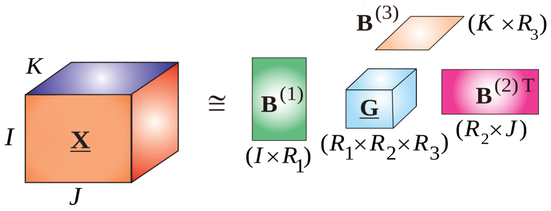
2.2. Tensor Decompositions

The application of tensor analysis to machine learning is a reasonable continuation of the artificial intelligence model development. The structure of such models satisfies the multilinear algebra properties, which allows the processing of more complex data. The conventional convolutional layers in neural networks can be identified via a low-rank tensor with the convolution operator. However, such a layer structure consumes a lot of computational time and resources. Therefore, one can use tensor decomposition methods to accelerate the corresponding convolutional neural networks.
Let us define the necessary notations and operations of tensor analysis [17]. Let X ̲ = [ x i 1 , , i N ] R I 1 × × I N be an N-order tensor. The mode-n unfolding of X ̲ is the rearrangement by mode-n fibers by constructing the columns of matrix X n = [ x i n , j ] R I n × p n I p for n { 1 , , N } , where j = 1 + k = 1 , k n N ( i k 1 ) j k with j k = m = 1 , m n k 1 I m , and i n = 1 , , I n . In a general case, one reshapes a tensor X ̲ into X n R p = 1 n I p × r = n + 1 N I r ( x i 1 , , i N x i , j ), where i = 1 + p = 1 n ( i p 1 ) m = 1 p 1 I m and j = 1 + r > n N ( i r 1 ) m = n + 1 r 1 I m . The next useful tensor operation is the mode- { n } product. Let U R J × I n , then Z ̲ = X ̲ × n U , where Z ̲ = [ z i 1 , , i n 1 , j , i n + 1 , , i N ] R I 1 , , I n 1 , J , I n + 1 , , I N and z i 1 , , i n 1 , j , i n + 1 , , i N = i n = 1 I n x i 1 , , i N u j , i n . The canonical polyadic decomposition transforms an N-order tensor X ̲ R I 1 × × I N into a linear combination of terms b r ( 1 ) b r ( N ) , which are first-order tensors such as
X ̲ r = 1 R λ r b r ( 1 ) b r ( N )
= Λ ̲ × 1 B ( 1 ) × 2 × N B ( N ) .
where λ r are non-zero entries of the diagonal core tensor Λ ̲ R R × × R and B ( n ) = [ b 1 ( n ) , , b R ( n ) ] R I n × R , and ∘ is the outer product. To clarify the concept, the CP decomposition of the three-order tensor is given in Figure 2.
As one can see from Figure 2, the three-order tensor X ̲ can be illustrated as the product of its three-order diagonalized core tensor Λ ̲ and B ( 1 ) , B ( 2 ) , and transposed B ( 3 ) matrices. Computing matrices and diagonalized core tensors separately is a less complex procedure than processing the full tensor format. The CP decomposition with the corresponding structure has the least computational complexity among other approaches.
Unlike the CP decomposition, the Tucker decomposition is a more general factorization of an Nth-order tensor into a small size, not-diagonalized core tensor and factors:
According to Figure 3, three-order tensor X ̲ is isomorphic to the product of its three-order core tensor G ̲ and B ( 1 ) , B ( 2 ) , and transposed B ( 3 ) matrices. Unlike the CP, Tucker decomposition contains full-format core tensor G ̲ , which raises the computational complexity of the solution.
X ̲ r 1 = 1 R 1 r N = 1 R N g r 1 , , r N b r 1 ( 1 ) b r N ( N )
= G ̲ × 1 B ( 1 ) × 2 × N B ( N ) ,
G ̲ R R 1 × × R N is the core tensor, and B ( n ) = [ b 1 ( n ) , , b R n ( n ) ] R I n × R n are the mode-n factor matrices, n = 1 , , N . In Figure 3, the Tucker decomposition of the three-order tensor is demonstrated.
Let X ̲ R I × × I be a N-th order tensor, and R denote the rank of the decomposition. To better illustrate the difference between the full tensor format, CP, and Tucker-decomposed layer, the evaluation of computational complexity is given in Table 1.
According to the calculations given in Table 1, the CP decomposition possesses lower computational complexity than Tucker. This can be explained by the diagonalization Λ ̲ of the core tensor G ̲ in Figure 2 and Figure 3. One should note that along with (1) and (2) decompositions, there exists a hierarchical Tucker (HT) [20] and tensor train (TT) [21]. These approaches require fewer hardware resources than Tucker decomposition and significantly accelerate the work of neural networks. However, the graph structure of HT and TT decompositions does not preserve the precision (accuracy) as the CP and Tucker approaches do. Also, if tensor decompositions reduce the number of computations, it will cause the precision loss. Therefore, it is necessary to use the positive–negative momentum optimization algorithms.

2.3. Optimization Algorithms

The quality of training in machine learning depends on the backward error propagation. In other words, precision, recall, and other metrics have high values if the loss function gives minimal values. The closer optimization algorithms descend to the global minimum, the higher the final precision is that can be achieved.
In paper [22], the authors introduced a regret-bound metric R ( T ) , which estimates the convergence rate of the optimization algorithm to the global minimum. The convergence rate metrics are defined as follows:
R ( T ) : = t = 1 T [ f t ( θ t ) f t ( θ * ) ] ,
where θ * = a r g m i n θ t = 1 T f t ( θ t ) , f t ( θ t ) is a continuous function and g 1 : T , i = ( g 1 , i , . . . , g T , i ) R T is the gradient in 1 , , T iterations and i-th dimension. The conventional optimization algorithms, namely, SGD and Adam, have the R ( T ) as O ( T ) . Such a metric means that the optimization algorithm is proper for machine learning models. Consider the Lebesgue norms L 2 ( R ) and L ( R ) , which have the corresponding norms:
g 1 : T , i 2 : = R g 1 : T , i 2 d θ t , i 1 / 2 G ,
θ n , i θ m , i 2 D ,
g 1 : T , i : = sup θ t , i R ( g 1 : T , i ) G ,
θ n , i θ m , i D ,
where G , D , R , D are positive real numbers and the indices are m , n { 1 , , T } . Next, we provide the positive–negative momentum optimization algorithm.
Let f : Ω R be a smooth function over a closed convex set Ω R n with n 2 that contains one or more extremes. From [23], we are reminded that the most applicable optimization algorithm is stochastic gradient descent
θ t + 1 = θ t α t f ( θ t ) ,
where θ t is a weight, α t is a learning rate, f ( θ t ) is a loss function, and f ( θ t ) is a gradient. This algorithm still finds application in modern neural networks. However, such an optimizer does not achieve the global minimum neighborhood of the objective function. This fact has been checked using test Rastrigin and Rosenbrock functions. Moreover, considering only the learning rate slows the minimization process because of non-dynamical updates. For that reason, the authors proposed Adam with exponential moving averages.
The main feature of the Adam optimizer is the utilization of exponential moving averages of the gradient and its square. Such an approach considers not only gradient directions but also means of moments. The Adam algorithm can be described by the following iterative formula
θ t = θ t 1 α t m ^ t v ^ t + ϵ ,
where
m ^ t = m t 1 β 1 t , v ^ t = v t 1 β 2 t ,
m t = β 1 m t 1 + ( 1 β 1 ) g t , v t = β 2 v t 1 + ( 1 β 2 ) g t 2 .
The parameters β 1 , β 2 are called moments, designed for m t and v t , respectively. Adam has the following regrets bound.
Theorem 1.
([22]). Let γ > 0 , β 1 , β 2 are moments, ϵ is a vanishing parameter, η = β 1 2 β 2 , λ ( 0 , 1 ) , and f t is a continuous convex function, whose g t and θ t with θ * satisfy the conditions (4)–(7). Then, Adam has the following regret-bound assessment:
R ( T ) D 2 T 2 γ ( 1 β 1 ) i = 1 n v T , i
+ γ ( 1 + β 1 ) G 3 G 2 ( 1 β 1 ) 1 β 2 ( 1 η ) 2 i = 1 T g 1 : T , i 2
+ D 2 G 1 β 2 2 γ ( 1 β 1 ) ( 1 λ ) 2 .
The exponential moment estimation accelerates the descent towards the extreme point. However, Adam cannot achieve the global minimum of objective function. Besides the local minimum avoidance problem, this optimizer does not handle the vanishing and exploding gradient issues, which impair the minimization process. This problem inspired us to propose optimization algorithms with positive–negative moment estimations. The DiffPNM was proposed in [15] as a majority voting ensemble learning model for increasing the accuracy of solving the pattern recognition problem in images from the UC-merced dataset. Such an approach is based on the positive–negative moment estimation, which is a more general technique than usual exponential moving averages. For considering the previous gradient values, DiffPNM utilizes the friction parameter
ξ t = 1 1 + exp ( | g t g t 1 | ) ,
which analyzes the nearest domain more precisely and broadly and helps to reach the global minimum of the loss function. The DiffPNM can be described as follows:
θ t = θ t 1 α t ξ t m ^ t ( v ^ t + ϵ ) ( 1 + β 0 2 ) + β 0 2 ,
where
m t = β 1 2 m t 1 + ( 1 β 1 2 ) g t ,
m ^ t = ( 1 + β 0 ) m t β 0 m t 1 1 β 1 t ,
v t = β 2 v t 1 + ( 1 β 2 ) g t 2 ,
v max = max ( v t , v max ) ,
v ^ t = v max 1 β 2 t .
This optimization algorithm contains the additional moment β 0 , which helps to build a more accurate direction towards a global minimum of the loss function.
Theorem 2.
Let α > 0 , β 0 , β 1 , β 2 are moments, ϵ is a vanishing parameter, ξ t is the friction coefficient, η = β 1 2 β 2 , λ ( 0 , 1 ) , and f t is continuous convex function, whose g t and θ t with θ * satisfy the regret bound conditions. Then, the DiffGrad has the following regret-bound assessment:
R ( T ) D 2 T 2 α ( 1 β 0 ) ( 1 β 1 ) 2 i = 1 d ( 1 + exp ( | g 1 , i | ) ) v ^ T , i
+ α ( 1 + β ) G 3 G 2 ( 1 β 0 ) ( 1 β 1 ) 2 ( 1 η ) 2 1 β 2 i = 1 d g 1 : t , i 2
+ D 2 G 1 β 2 2 α i = 1 d β ( 1 β 0 ) ( 1 β 1 ) 2 ( 1 λ ) 2 .
The YogiPNM described in paper [16] shows the best results in solving the pattern recognition problem on skin lesion image datasets. Like DiffPNM, this optimization algorithm relies on the positive–negative moment estimation technique and adjusting the learning rate update. Such an optimizer has the transformed second moment v t by defining a more accurate gradient direction instead of considering that it does not contain the additional parameters. The YogiPNM is defined by the following formula:
θ t = θ t 1 α t m ^ t ( v ^ t + ϵ ) ( 1 + β 0 2 ) + β 0 2 ,
where
m t = β 1 2 m t 1 + ( 1 β 1 2 ) g t ,
m ^ t = ( 1 + β 0 ) m t β 0 m t 1 1 β 1 t ,
v t = β 2 v t 1 + ( 1 β 2 ) s i g n ( u t 1 g t 2 ) g t 2 ,
v max = max ( v t , v max ) ,
v ^ t = v max 1 β 2 t .
Theorem 3.
Let α > 0 , β 0 , β 1 , β 2 be moments, ϵ a vanishing parameter, η = β 1 2 β 2 , λ ( 0 , 1 ) , and f t the continuous convex function, whose g t and θ t with θ * satisfy the regret bound conditions. Then, the YogiPNM has the following regret-bound assessment:
R ( T ) D 2 T 2 α ( 1 β 0 ) ( 1 β 1 ) 2 i = 1 d v ^ T , i
+ α ( 1 + β ) G 3 G 2 ( 1 β 0 ) ( 1 β 1 ) 2 ( 1 η ) 2 1 β 2 i = 1 d g 1 : t , i 2
+ D 2 G 1 β 2 2 α i = 1 d β ( 1 β 0 ) ( 1 β 1 ) 2 ( 1 λ ) 2 .
Like YogiPNM, PNMBelief [16] shows good results in skin disease classification problems. Its main feature is the learning rate adaptation considering the “belief” in the current gradient direction. There is a difference between PNMBelief and YogiPNM in parameters v t and s t , which are defined as exponential moving averages of g t 2 and ( g t m t ) 2 , respectively. Considering s t as the prediction of the gradient at the next time step, if the observed gradient greatly deviates from the prediction, then the algorithm distrusts the current observation and takes a small step; if the observed gradient is close to the prediction, it can be trusted and a large step can be taken.
θ t = θ t 1 α t m ^ t ( s ^ t + ϵ ) ( 1 + β 0 2 ) + β 0 2 ,
where
m t = β 1 2 m t 1 + ( 1 β 1 2 ) g t ,
m ^ t = ( 1 + β 0 ) m t β 0 m t 1 1 β 1 t ,
s t = β 2 s t 1 + ( 1 β 2 ) ( g t m t ) 2 g t 2 ,
s max = max ( s t , s max ) ,
s ^ t = s max 1 β 2 t .
Theorem 4.
Let α > 0 , β 0 , β 1 , β 2 be moments, ϵ a vanishing parameter, η = β 1 2 β 2 , λ ( 0 , 1 ) , and f t the continuous convex function, whose g t and θ t with θ * satisfy the regret bound conditions. Then, the PNMBelief has the following regret-bound assessment:
R ( T ) D 2 T 2 α ( 1 β 0 ) ( 1 β 1 ) 2 i = 1 d v ^ T , i
+ α ( 1 + β ) G 3 G 2 1 + log T ( 1 β 0 ) ( 1 β 1 ) 2 ( 1 η ) 2 1 β 2 i = 1 d g 1 : t , i 2
+ D 2 G 1 β 2 2 α i = 1 d β ( 1 β 0 ) ( 1 β 1 ) 2 ( 1 λ ) 2 .
Positive–negative momentum optimization algorithms showed their ability to increase the quality of solving pattern recognition problems in multi-modal [16] and ensemble neural networks [15]. Considering the properties of DiffPNM, YogiPNM, and PNMBelief in an ensemble network containing factorized convolutional layers, we can decrease the precision loss while solving the object detection problem.

3. Proposed Yolov8-CP-Astrid and Yolov8-Tucker-2 Neural Networks
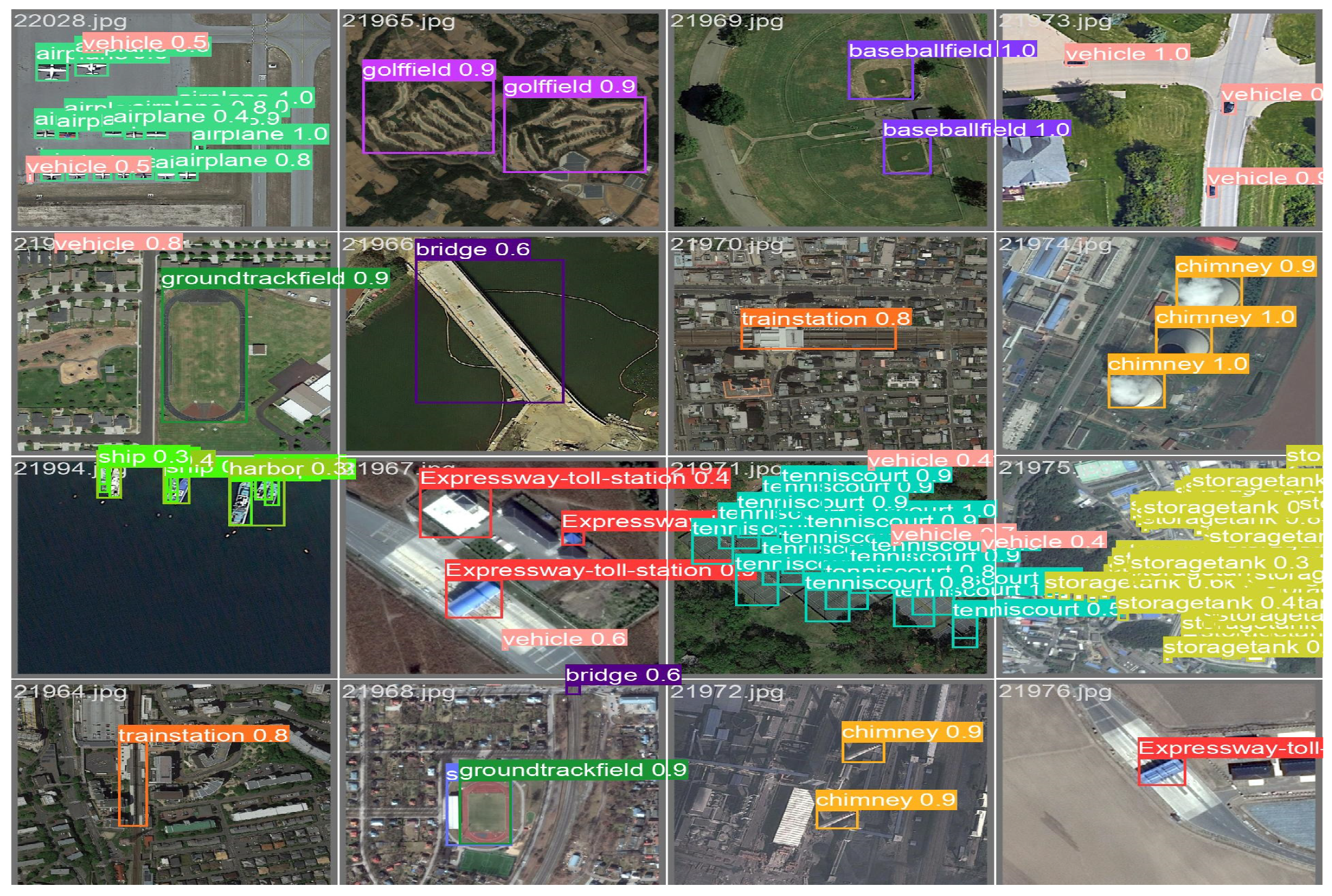
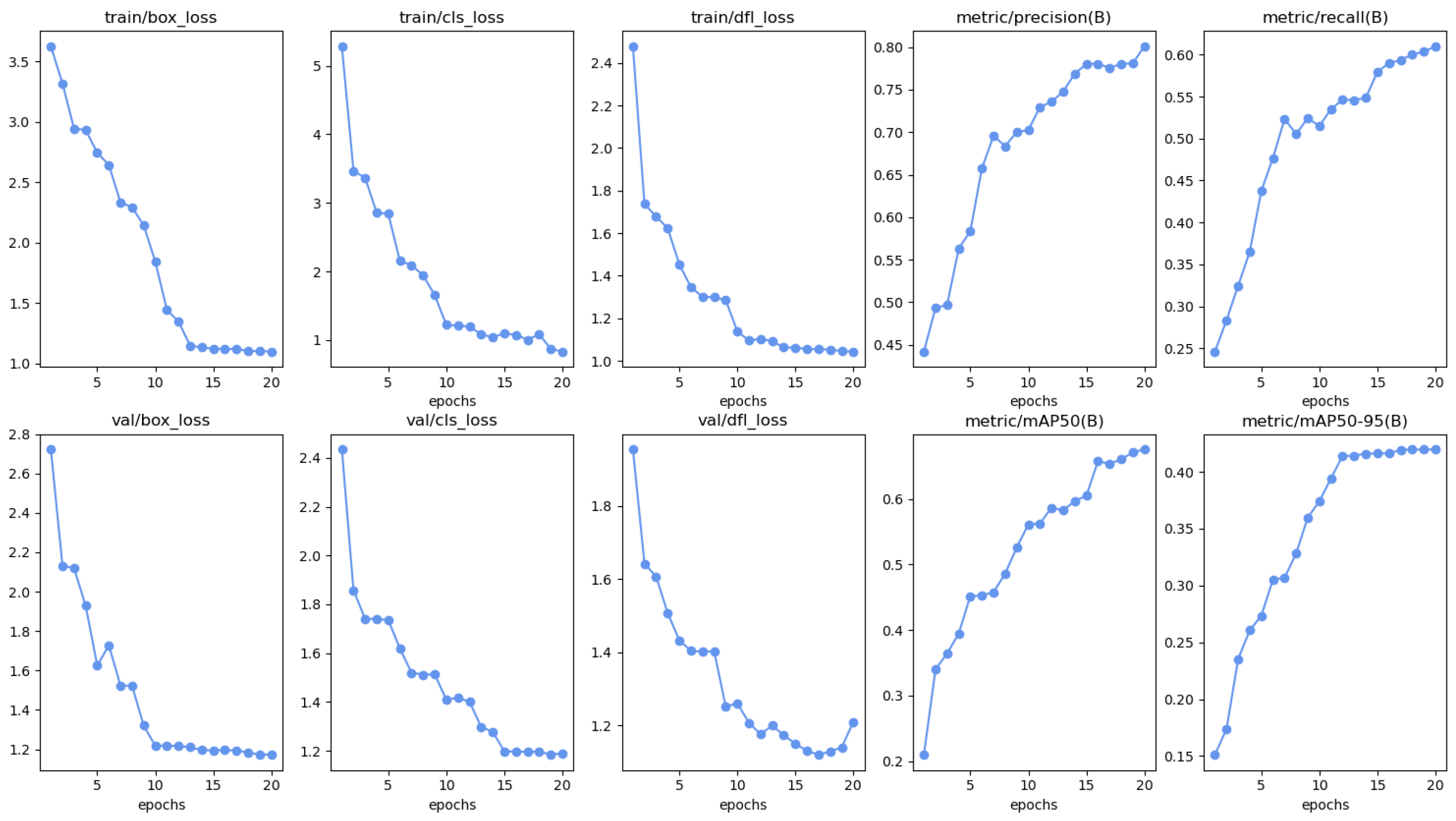
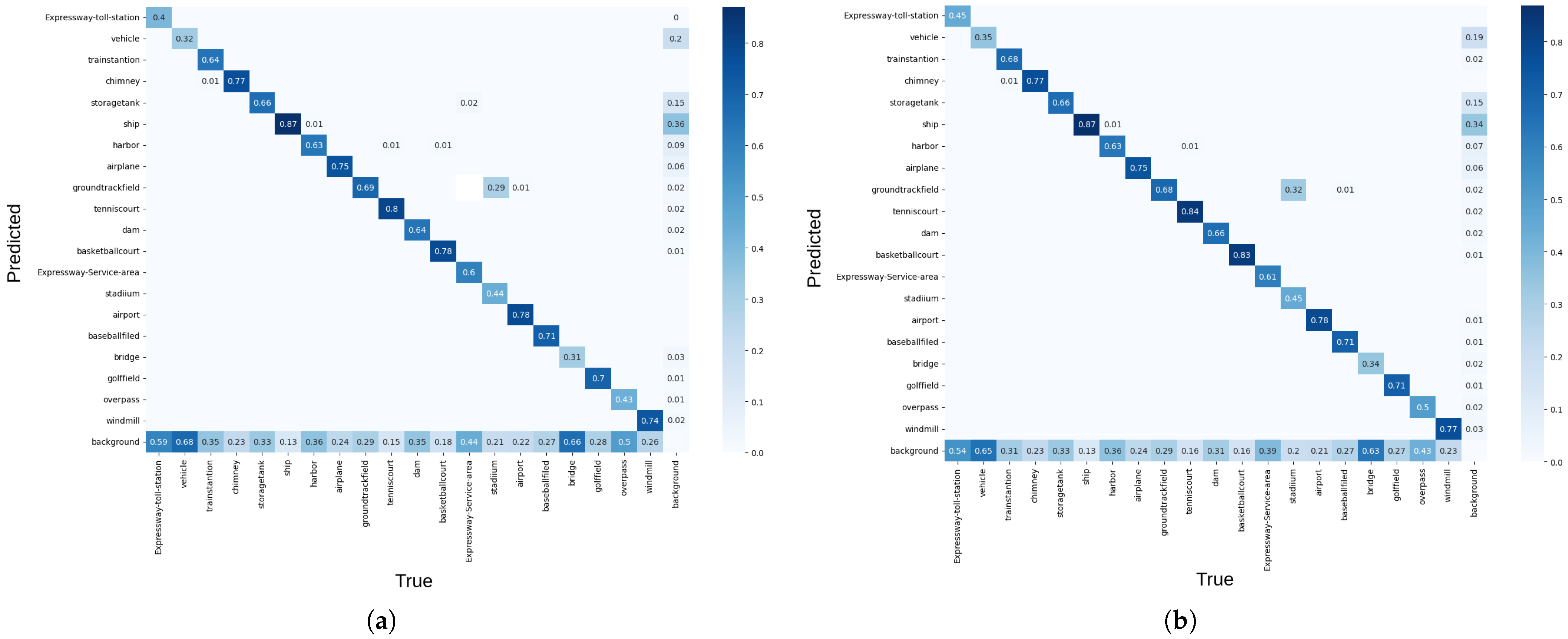
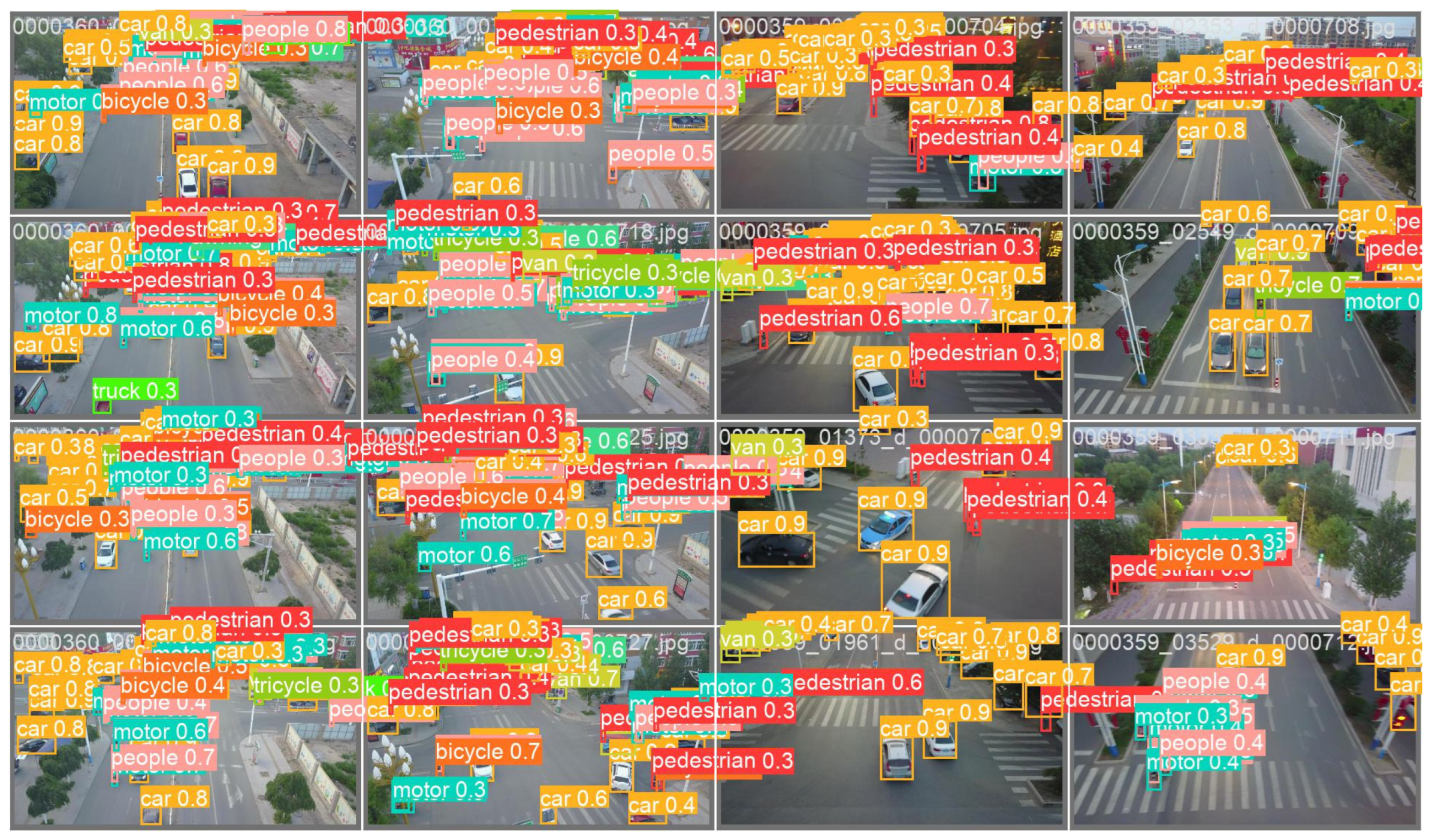
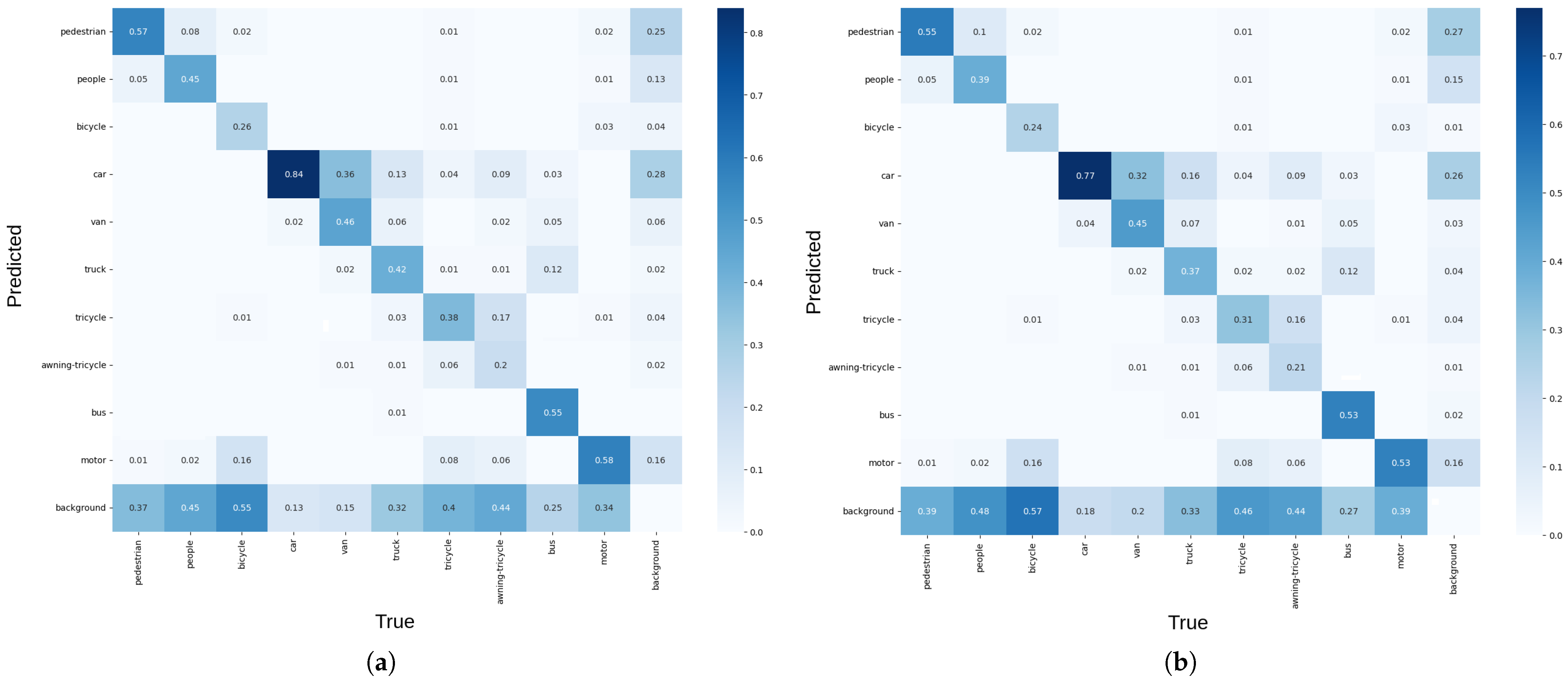
The Yolov8 architecture consists of many convolutional layers in the backbone, neck, and head blocks, as shown in Figure 1. These three blocks contain the Conv, SPPF, Bootleneck, C2f, and detect modules. The kernel in each Yolov8 convolution layer is represented by the fourth-order tensor W ̲ R T × C × D 1 × D 2 , where T and C are the number of output and input channels, and D 1 and D 2 are the size of the filter. In many deep convolutional neural networks, kernels process much redundant information. Therefore, we approximate the kernel tensors by lower-rank structures obtained from various tensor decompositions. To accelerate the training process, we decompose these layers into blocks of sub-layers of a smaller shape. The decomposition of the Conv2d layer is made using the CP-Astrid [24] and Tucker-2 schemes [25], shown in Figure 4 and Figure 5.
In the Yolov8 network, we factorize the Conv2d convolutional layers by CP-Astrid and Tucker-2 decompositions. Next, we substitute the compressed Conv2d layer in Conv, Bootleneck, SPPF, C2f, and Detect blocks from Figure 1. One may use CP-Lebedev and Tucker-2-CP in Yolov8, but these factorization models reduce many more computations that negatively impact the preservation of precision (accuracy). Considering the Figure 4, the full tensor X ̲ R T × C × D 1 × D 2 is Conv2d layer. In the case of CP decomposition, we apply Astrid’s scheme to X ̲ R T × C × D 1 × D 2 and receive three sublayers X ̲ 1 R R × C × 1 × 1 , X ̲ 2 R R × R × D 1 × D 2 , and X ̲ 3 R T × R × 1 × 1 . One should note that the tensor X 2 ̲ R R × R × D 1 × D 2 is the tensor product of X ̲ 2 ( 1 ) R R × R × D 1 × 1 and X ̲ 2 ( 2 ) R R × R × 1 × D 2 . In [26], the authors noticed this fact and proposed the CP-Lebedev decomposition, which is based on factorization of Conv2d tensor X ̲ into X ̲ 1 R R × C × 1 × 1 , X ̲ 2 ( 1 ) R R × R × D 1 × 1 , X ̲ 2 ( 2 ) R R × R × 1 × D 2 , and X ̲ 3 R T × R × 1 × 1 . In the case of Tucker decomposition, we use the Tucker-2 layer decomposition model, which divides X ̲ R T × C × D 1 × D 2 into X ̲ 1 R R 1 × C × 1 × 1 , X ̲ 2 R R 2 × R 1 × D 1 × D 2 , and X ̲ 3 R T × R 2 × 1 × 1 . Using the CP-Astrid scheme to the sublayer X ̲ 2 R R 2 × R 1 × D 1 × D 2 , we obtain X ̲ 2 ( 1 ) R R × R 1 × 1 × 1 , X ̲ 2 ( 2 ) R R × R × D 1 × D 2 , and X ̲ 2 ( 3 ) R R 2 × R × 1 × 1 , which transforms the Tucker decomposition into Tucker-CP analog [27]. In practice, it is usually considered that D = D 1 = D 2 . Let I 1 and I 2 be the height and width of the input image, respectively. Suppose I ^ 1 and I ^ 2 are the reduced height and width after using the convolution operation. For clearness, we list the computational complexities of the layer factorizations in Table 2.
Let us substitute the blocks of the Yolov8 architecture, such as Conv, SPPF, BootleNeckm C2f, and Detect, in convolutional layer decomposition models shown in Figure 6 and Figure 7. The convolution can be presented as the mapping X ̲ R T × C × I Y ̲ R T × C × O by the following formula:
y t , c , o = t = 1 T c = 1 C i = 1 I w t t + 1 , c c + 1 , i , o x t , c , i ,
where T is the height, C is the width, and I is the number of channels of the input data. Analogically, T is the height, C is the width, and O is the number of channels of the output data. Next, we decompose the tensor W ̲ via the Tucker-2 model and obtain the following equation:
w t , c , i , o = r 1 = 1 R 2 r 2 = 1 R 2 r 3 = 1 R 3 g r 1 , r 2 , r 3 b t , r 1 ( 1 ) b c , r 2 ( 2 ) b o , r 3 ( 3 ) ,
where [ g r 1 , r 2 , r 3 ] = G ̲ is the core tensor of shape ( R 1 × R 2 × R 3 ) and [ b t , r 1 ( 1 ) ] = B ( 1 ) R T × R 1 , [ b c , r 2 ( 2 ) ] = B ( 2 ) R C × R 2 , and [ b o , r 3 ( 3 ) ] = B ( 3 ) R O × R 3 are the factor matrices. Next, we incorporate the convolutional layer decomposition (17) into the Yolov8 architecture (Figure 1). We will denote such an architecture as the Yolov8-Tucker-2 neural network.
In the case of CP-Astrid decomposition, we have the following decomposition of W ̲ :
w t , c , i , o = r 1 = 1 R r 2 = 1 R r 3 = 1 R λ r 1 , r 2 , r 3 b t , r 1 ( 1 ) b c , r 2 ( 2 ) b o , r 3 ( 3 ) ,
where the core tensor Λ ̲ = d i a g ( G ̲ ) . Next, we use the convolutional layer decomposition at each module of the Yolov8 architecture. We call this model Yolov8-CP-Astrid.
The proposed Yolov8-Tucker-2 and Yolov8-CP-Astrid architectures are designed to accelerate the solution of the object detection problem. However, it is necessary to reduce the precision and recall losses caused by simplifying the convolutional layers at each Yolov8 module. We address this issue with positive–negative momentum optimizers DiffPNM, YogiPNM, and PNMBelief. The majority of modern neural networks utilize conventional optimization algorithms, such as SGD and Adam. These approaches are still relevant for loss function minimization, which can be found in the backpropagation process. However, these optimization algorithms do not guarantee the achievement of the global minimum of the loss function. Therefore, it is necessary to use DiffPNM, YogiPNM, and PNMBelief, which operate with positive–negative momentum estimation. This technique has proven its superiority over existing basic optimization algorithms in [15] and enables us to achieve the global minimum for a smaller number of epochs (iteration), which speeds up the training process.

4. Results

In this section, we examine the training process of the compressed Yolov8 neural network, containing positive–negative momentum optimizers and tensor decomposition models. The training process is investigated while solving the object detection problem in images from the DIOR dataset.
For the program implementation of the Yolov8 architecture and positive–negative momentum optimizers, we use the PyTorch 1.11 library of Python 3.9.3. For the realization of CP and Tucker decompositions, we use the TensorLy library [28].The splits were originally 50% train and 50% test sample. We made a few changes by keeping the 50% train for only training and splitting the test dataset to 20–80% for validation and testing parts. The number of epochs equals 20. The learning rate α = 0.001 , the moments β 0 = 0.9 , β 1 = 0.999 , β 2 = 0.999 , ϵ = 1 × 10 8 , and the weight decay is 0. For better reinforcement, we use weight decoupling and the amsgrad procedure. The training process is implemented in NVIDIA Tesla T4, PCIe 3.0, 16 GiB GDDR6, 256 bit, and GPU 585 MHz. The rank of CP and Tucker decomposition is 100. In Table 3, we present a list of the results of solving the object detection problem in images from the DIOR dataset [29] by full tensor format and compressed Yolov8 models with SGD, Adam, DiffPNM, YogiPNM, and PNMBelief.
Considering the results shown in Table 3, one can see that the training of conventional Yolov8 models requires 24,119.94–24,503.03 s. In this case, the DiffPNM achieves the highest precision and recall values 86.305 % and 63.841 % with the least values of box, class, and distribution focal losses, which have the values 0.894 , 0.428 , 0.930 , respectively. For 24,283.95 s, the YogiPNM achieves precision and recall with values 86.262 % and 63.517 % , respectively. The box, class, and distribution focal losses are 0.917 , 0.520 , and 0.946 . The PNMBelief lets the Yolov8 model solve the object detection problem in images from the DIOR dataset with lower precision and recall.
The SGD and Adam achieved the worst precision and recall, regardless of the smaller time costs. In the case of training the Yolov8-CP-Astrid model, the best precision and recall were achieved by YogiPNM with values 82.050 % and 60.109 % for 11,501.01 s. The DiffPNM and PNMBelief demonstrated the second and third results in precision and recall, respectively. The SGD and Adam achieved less precision and recall value because of the inferior loss function minimization. For the Yolov8-Tucker-2 model, the DiffPNM received the best precision and recall values, 82.885 % and 60.881 % , respectively. The YogiPNM achieved almost the same results in precision and recall as DiffPNM, 82.843 % and 60.811 % , respectively. The precision and recall achieved by PNMBelief are 82.045 % and 60.292 % . From Figure 8 and Figure 9, one can see that the Yolov8-Tucker-2 with DiffPNM obtained almost the same results as Yolov8 with DiffPNM. However, the proposed neural network does not have distinct train stations and finds false vehicles on 21964 images. In image 21972, the proposed Yolov8-Tucker-2 does not find chimneys and accepts the false building as a train station. In image 21966, the proposed models detected the same bridge twice and discovered a false harbor. In other cases, the proposed Yolov8-Tucker-2 network detects the objects correctly.
Next, in Figure 10 and Figure 11, we demonstrate the per epochs via train and validation bounded box, class and distribution focal loss functions, precision, recall, mAP50(B), and mAP50-95(B).
Figure 12 demonstrates normalized confusion matrices obtained by testing Yolov8 with DIffPNM and Yolov8-Tucker-2 using DiffPNM for identifying detected objects in images from the DIOR dataset.
We considered expanding the study by solving the object detection problem on the VisDrone 2020 dataset, which contains 10 classes of objects. However, the images in this dataset often contain small objects, such as people, bicycles, and motorcycles, which are challenging to detect using considered approaches.
Analyzing the results given in Table 4, one can notice that Yolov8 requires 9433.42–9587.94 s for training. The DiffPNM achieves the highest precision and recall values 79.372 % and 30.084 % with the lowest values of box, class, and distribution focal losses, which have the values 1.084 , 0.844 , 1.159 , respectively. Next, the YogiPNM receives precision and recall, 79.344 % and 30.084 % , respectively. The box, class, and distribution focal losses have values of 1.126 , 0.884 , and 1.190 . The rest of the optimizers show results with greater values of losses and lower values of precision and recall. The Yolov8-CP-Astrid model with DiffPNM gives precision and recall with values 72.571 % and 36.463 % for 5894.03 s. The YogiPNM and PNMBelief have the second and third results in precision and recall, respectively. The rest of the state-of-the-art optimizers provide less precision and recall values. In the case of the Yolov8-Tucker-2 model, the YogiPNM received the best precision and recall values, 74.788 % and 27.914 % , respectively. The second and third results in precision and recall were achieved by DiffPNM and PNMBeleif. Other optimizers demonstrate the results with lower precision and recall. Several images with object detection frames are shown in Figure 13 and Figure 14.
Considering Figure 13 and Figure 14, one can see that the Yolov8-Tucker-2 with DiffPNM achieved almost the same results as Yolov8 with DiffPNM. However, the neural network was not able to distinguish between small vehicles and people, bicycles and pedestrians, and trucks and vans.
Next, in Figure 15 and Figure 16, we demonstrate the per epochs via train and validation bounded box, class and distribution focal loss functions, precision, recall, mAP50(B), and mAP50-95(B).
Figure 17 shows normalized confusion matrices resulting from testing Yolov8 with DIffPNM and Yolov8-Tucker-2 with DiffPNM, respectively, for identifying detected objects in images from the VisDrone 2020 dataset.
The proposed Yolov-CP-Astrid and Yolov8-Tucker-2 neural network with DiffPNM, YogiPNM, and PNMBeleif achieved better results than the conventional Yolov8 with SGD and Adam. The proposed neural network architectures are faster than the SOTA model by 44–52% and increase the precision and recall by 0.84–0.94 and 0.228–1.07 percentage points, respectively.
The proposed Yolov8n with tensor decompositions and advanced optimization algorithms is able to solve objected detection problems on DIOR and VisDrone-2020 datasets as successfully as state-of-the-art models do. Our model shows mAP 68.14 % , which is greater than Bayes R-CNN [30], with the following backbones: ResNet-50, ResNext-50, ShuffleNet, MobileNet V3-L. However, RegNet and MRENet show mAP values of 71.77 % and 73.91 % , respectively. The R-CNN model with comprehensive learning techniques attained the mAP of 74.37 % on the DIOR [31]. An accelerated Yolov8n by tensor decompositions outperforms the EfficientDet in mAP on DIOR dataset [32]. The majority of considered state-of-the-art neural networks do not solve the object detection problem on the DIOR dataset better than accelerated Yolov8n with a positive–negative momentum optimizer. Meanwhile, RegNet and MRENet with tensor decompositions can preserve the accuracy of solving object detection problems. Considering the models of this object detection problem in VisDrone 2020, many studies contain the training using Yolo-based models [33,34]. However, Yolov8n has many modifications that show greater precision and mAP, such as Yolov8s, Yolov8m, Yolov8s, and Yolov8x. As the next possible research focus, it could be useful to apply tensor decompositions and advanced optimization algorithms to later Yolo-based and other perspective ANN models.

5. Discussion

Based on the results given in Table 3, it can be claimed that the tensor decomposition technique accelerates the training of neural networks while solving the object detection problem on the DIOR dataset. Table 5 represents the evolution of artificial neural networks with application to object detection problem.
The use of such advanced optimization algorithms allows the minimization of the precision and recall losses, which happen because of the convolutional layer decomposition in Conv, SPPF, BootleNeck, C2f, and Detect in Yolov8.
The comparison of conventional Yolov8 with SGD or Adam with Yolov8-CP-Astrid or Yolov8v-Tucker-2 with positive–negative momentum approaches shows that these advanced architectures outperform existing ones in speed, precision, and recall. One of the known shortcomings is that the proposed model fails to correctly detect objects like train stations, chimneys, and buildings in the DIOR dataset. The same problem can be found in the VisDrone 2020 dataset, where the proposed model sometimes confuses people with small vehicles, and vans can be confused with trucks. This issue can be explained by analyzing the entire figure via conventional convolutional layers. The advanced optimizers increased the precision and recall of Yolov8n and its accelerated models by CP and Tucker decompositions. The solution to this problem is the utilization of a transformer neural network, based on the self-attention layer. Also, the ensemble learning techniques can enhance the final precision of solving object detection problems on multiclass datasets. This fact makes the foundation for further exploring the combination of optimization algorithms and tensor decompositions. For example, the utilization of hierarchical Tucker [20], ADA-Tucker [39], singular value [40], and tensor-train [21] decomposition in neural networks can simplify its structure with minimal loss of final precision. Moreover, it is possible to reinforce such models with optimization algorithms, such as fractional-order [41], information-geometric [42], hybrid [43], and other metaheuristic [44] approaches.

6. Conclusions

Further studies can be devoted to compressing not just the deep convolutional but physics-informed, complex-valued, quantum, and graph neural networks. Along with the CP-Astrid and Tucker-2 decomposition models, we will use the tensor-train, hierarchical Tucker, and singular value decomposition, with the intent to accelerate the neural network training with minimal loss of accuracy. We also plan to modify positive–negative approaches using fractional derivatives or combination with population-based approaches. By involving the Riemann–Liouville, Caputo, and Grunwald–Letnikov fractional rational derivatives [45], the optimization process can take a lower number of epochs, which may also reduce the training time. Similarly, the hybrid approaches, like AdaSwarm [46], can significantly improve the quality of neural network performance. The use of information-geometric optimization algorithms, natural [47], and mirror [48] gradient descent can integrate the classical tensor decomposition into quantum machine learning [49].

Author Contributions

Conceptualization, P.L. and N.N.; methodology, P.L. and D.B.; software, R.A., D.R., A.B. and D.K.; validation, R.A., D.R., D.B. and A.B.; formal analysis, R.A.; investigation, R.A.; resources, D.K. and D.B.; data curation, R.A. and A.B.; writing—original draft preparation, R.A. and N.N.; writing—review and editing, R.A., N.N., P.L. and D.B.; visualization, R.A., D.R. and D.K.; supervision, P.L.; project administration, P.L.; funding acquisition, D.K. and N.N. All authors have read and agreed to the published version of the manuscript.

Funding

The research reported in Section 3 was supported by the Russian Science Foundation (Project No. 24-71-10016). The rest of the paper was supported by the Russian Science Foundation (Project No. 24-71-00024).

Data Availability Statement

The link to the code can be found here: https://github.com/Ruslan26reg/Yolov8-tensor-decomposition-and-advanced-optimizers.git, accessed on 12 February 2025.

Conflicts of Interest

The authors declare no conflicts of interest.

References

  1. Tzeng, Y.C.; Chen, K.S.; Kao, W.-L.; Fung, A.K. A dynamic learning neural network for remote sensing applications. IEEE Trans. Geosci. Remote Sens. 1994, 32, 1096–1102. [Google Scholar] [CrossRef]
  2. Xia, N.; Cheng, L.; Li, M. Mapping Urban Areas Using a Combination of Remote Sensing and Geolocation Data. Remote Sens. 2019, 11, 1470. [Google Scholar] [CrossRef]
  3. Li, A.S.; Chirayath, V.; Segal-Rozenhaimer, M.; Torres-Pérez, J.L.; van den Bergh, J. NASA NeMO-Net’s Convolutional Neural Network: Mapping Marine Habitats with Spectrally Heterogeneous Remote Sensing Imagery. IEEE J. Sel. Top. Appl. Earth Obs. Remote Sens. 2020, 13, 5115–5133. [Google Scholar] [CrossRef]
  4. Wu, C.; Lou, Y.; Wang, L.; Li, J.; Li, X.; Chen, G. SPP-CNN: An Efficient Framework for Network Robustness Prediction. IEEE Trans. Circuits Syst. I 2023, 70, 4067–4079. [Google Scholar] [CrossRef]
  5. Adla, D.; Reddy, G.V.R.; Nayak, P.; Karuna, G. A full-resolution convolutional network with a dynamic graph cut algorithm for skin cancer classification and detection. Healthc. Anal. 2023, 3, 100154. [Google Scholar] [CrossRef]
  6. Li, Y.; Fan, Q.; Huang, H.; Han, Z.; Gu, Q. A Modified YOLOv8 Detection Network for UAV Aerial Image Recognition. Drones 2023, 7, 304. [Google Scholar] [CrossRef]
  7. Bagherzadeh, S.A.; Asadi, D. Detection of the ice assertion on aircraft using empirical mode decomposition enhanced by multi-objective optimization. Mech. Syst. Signal Process. 2017, 88, 9–24. [Google Scholar] [CrossRef]
  8. Gawlikowski, J.; Tassi, C.R.N.; Ali, M.; Lee, J.; Humt, M.; Feng, J.; Kruspe, A.; Triebel, R.; Jung, P.; Roscher, R.; et al. A survey of uncertainty in deep neural networks. Artif. Intell. Rev. 2023, 56, 1513–1589. [Google Scholar] [CrossRef]
  9. Marinó, G.C.; Petrini, A.; Malchiodi, D.; Frasca, D. Deep neural networks compression: A comparative survey and choice recommendations. Neurocomputing 2023, 520, 152–170. [Google Scholar] [CrossRef]
  10. Cheng, H.; Zhang, M.; Shi, J.Q. A Survey on Deep Neural Network Pruning: Taxonomy, Comparison, Analysis, and Recommendations. IEEE Trans. Pattern Anal. Mach. Intell. 2024, 46, 10558–10578. [Google Scholar] [CrossRef]
  11. Zhao, Y.; Wang, D.; Wang, L. Convolution Accelerator Designs Using Fast Algorithms. Algorithms 2019, 12, 112. [Google Scholar] [CrossRef]
  12. Ozaki, K.; Ogita, T.; Oishi, S.I.; Rump, S.M. Error-free transformations of matrix multiplication by using fast routines of matrix multiplication and its applications. Numer. Algorithms 2012, 59, 95–118. [Google Scholar] [CrossRef]
  13. Wu, Q.; Jiang, Z.; Hong, K.; Liu, H.; Yang, L.T.; Ding, J. Tensor-Based Recurrent Neural Network and Multi-Modal Prediction with Its Applications in Traffic Network Management. IEEE Trans. Netw. Serv. Manag. 2021, 18, 780–792. [Google Scholar] [CrossRef]
  14. Giraud, M.; Itier, V.; Boyer, R.; Zniyed, Y.; de Almeida, A.L. Tucker Decomposition Based on a Tensor Train of Coupled and Constrained CP Cores. IEEE Signal Process. Lett. 2023, 30, 758–762. [Google Scholar] [CrossRef]
  15. Abdulkadirov, R.; Lyakhov, P.; Bergerman, M.; Reznikov, D. Satellite image recognition using ensemble neural networks and difference gradient positive-negative momentum. Chaos Solitons Fractals 2024, 179, 114432. [Google Scholar] [CrossRef]
  16. Lyakhov, P.A.; Lyakhova, U.A.; Abdulkadirov, R.I. Non-convex optimization with using positive-negative moment estimation and its application for skin cancer recognition with a neural network. Comput. Opt. 2024, 48, 260–271. [Google Scholar] [CrossRef]
  17. Ji, Y.; Wang, Q.; Li, X.; Liu, J. A Survey on Tensor Techniques and Applications in Machine Learning. IEEE Access 2019, 7, 162950–162990. [Google Scholar] [CrossRef]
  18. Boizard, M.; Boyer, R.; Favier, G.; Cohen, J.E.; Comon, P. Performance estimation for tensor CP decomposition with structured factors. In Proceedings of the 2015 IEEE International Conference on Acoustics, Speech and Signal Processing (ICASSP), South Brisbane, QLD, Australia, 19–24 April 2015; pp. 3482–3486. [Google Scholar]
  19. Jang, J.-G.; Kang, U. D-Tucker: Fast and Memory-Efficient Tucker Decomposition for Dense Tensors. In Proceedings of the 2020 IEEE 36th International Conference on Data Engineering (ICDE), Dallas, TX, USA, 20–24 April 2020; pp. 1850–1853. [Google Scholar]
  20. Gabor, M.; Zdunek, R. Compressing convolutional neural networks with hierarchical Tucker-2 decomposition. Appl. Soft Comput. 2023, 132, 109856. [Google Scholar] [CrossRef]
  21. Oseledets, I.V. Tensor-train decomposition. SIAM J. Sci. Comput. 2011, 33, 2295–2317. [Google Scholar] [CrossRef]
  22. Kingma, D.P.; Ba, J. Adam: A Method for Stochastic Optimization. arXiv 2015, arXiv:1412.6980. [Google Scholar]
  23. Singh, N.; Data, D.; George, J.; Diggavi, S. SQuARM-SGD: Communication-Efficient Momentum SGD for Decentralized Optimization. IEEE J. Sel. Areas Inf. Theory 2021, 2, 954–969. [Google Scholar] [CrossRef]
  24. Astrid, M.; Lee, S.-I.; Seo, B.-S. Rank selection of CP-decomposed convolutional layers with variational Bayesian matrix factorization. In Proceedings of the 2018 20th International Conference on Advanced Communication Technology (ICACT), Chuncheon, Republic of Korea, 11–14 February 2018; pp. 347–350. [Google Scholar]
  25. Han, Y.; Lin, Q.H.; Kuang, L.D.; Gong, X.F.; Cong, F.; Wang, Y.P.; Calhoun, V.D. Low-Rank Tucker-2 Model for Multi-Subject fMRI Data Decomposition with Spatial Sparsity Constraint. IEEE Trans. Med. Imaging 2022, 41, 667–679. [Google Scholar] [CrossRef] [PubMed]
  26. Phan, A.-H.; Sobolev, K.; Sozykin, K.; Ermilov, D.; Gusak, J.; Tichavskỳ, P.; Glukhov, V.; Oseledets, I.; Cichocki, A. Stable low-rank tensor decomposition for compression of convolutional neural network. Lect. Notes Comput. Sci. 2020, 12374, 522–539. [Google Scholar]
  27. Lebedev, V.; Ganin, Y.; Rakhuba, M.; Oseledets, I.; Lempitsky, V. Speeding up convolutional neural networks using fine-tuned cp-decomposition. arXiv 2024, arXiv:1412.6553. [Google Scholar]
  28. Kossaifi, J.; Panagakis, Y.; Anandkumar, A.; Pantic, M. TensorLy: Tensor Learning in Python. J. Mach. Learn. Res. 2019, 20, 1–6. [Google Scholar]
  29. Wang, H.; Jiang, H.; Sun, J.; Zhang, S.; Chen, C.; Hua, X.S.; Luo, X. DIOR: Learning to Hash with Label Noise via Dual Partition and Contrastive Learning. IEEE Trans. Knowl. Data Eng. 2024, 36, 1502–1517. [Google Scholar] [CrossRef]
  30. Sharifuzzaman, S.A.S.M.; Tanveer, J.; Chen, Y.; Chan, J.H.; Kim, H.S.; Kallu, K.D.; Ahmed, S. Bayes R-CNN: An Uncertainty-Aware Bayesian Approach to Object Detection in Remote Sensing Imagery for Enhanced Scene Interpretation. Remote Sens. 2024, 16, 2405. [Google Scholar] [CrossRef]
  31. Sagar, A.S.; Chen, Y.; Xie, Y.; Kim, H.S. MSA R-CNN: A comprehensive approach to remote sensing object detection and scene understanding. Expert Syst. Appl. 2024, 241, 122788. [Google Scholar] [CrossRef]
  32. Ye, Y.; Ren, X.; Zhu, B.; Tang, T.; Tan, X.; Gui, Y.; Yao, Q. An Adaptive Attention Fusion Mechanism Convolutional Network for Object Detection in Remote Sensing Images. Remote Sens. 2022, 14, 516. [Google Scholar] [CrossRef]
  33. Zhan, W.; Sun, C.; Wang, M.; She, J.; Zhang, Y.; Zhang, Z.; Sun, Y. An improved Yolov5 real-time detection method for small objects captured by UAV. Soft Comput. 2022, 26, 361–373. [Google Scholar] [CrossRef]
  34. Alhawsawi, A.N.; Khan, S.D.; Rehman, F.U. Enhanced YOLOv8-Based Model with Context Enrichment Module for Crowd Counting in Complex Drone Imagery. Remote Sens. 2024, 16, 4175. [Google Scholar] [CrossRef]
  35. Li, H.; Huang, Y.; Zhang, Z. An Improved Faster R-CNN for Same Object Retrieval. IEEE Access 2017, 5, 13665–13676. [Google Scholar] [CrossRef]
  36. Chen, S.; Miao, Z.; Chen, H.; Mukherjee, M.; Zhang, Y. Point-attention Net: A graph attention convolution network for point cloudsegmentation. Appl. Intell. 2023, 53, 11344–11356. [Google Scholar] [CrossRef]
  37. Yang, C.; Kong, X.; Cao, Z.; Peng, Z. Cirrus Detection Based on Tensor Multi-Mode Expansion Sum Nuclear Norm in Infrared Imagery. IEEE Access 2020, 8, 149963–149983. [Google Scholar] [CrossRef]
  38. Sun, Y.; Yang, J.; Long, Y.; Shang, Z.; An, Z. Infrared Patch-Tensor Model with Weighted Tensor Nuclear Norm for Small Target Detection in a Single Frame. IEEE Access 2018, 6, 76140–76152. [Google Scholar] [CrossRef]
  39. Zhong, Z.; Wei, F.; Lin, Z.; Zhang, C. ADA-Tucker: Compressing deep neural networks via adaptive dimension adjustment tucker decomposition. Neural Netw. 2019, 110, 104–115. [Google Scholar] [CrossRef] [PubMed]
  40. Denton, E.L.; Zaremba, W.; Bruna, J.; Cun, Y.L.; Fergus, R. Exploiting linear structure within convolutional networks for efficient evaluation. In Proceedings of the NIPS’14: Proceedings of the 28th International Conference on Neural Information Processing Systems, Montreal, QC, Canada, 8–13 December 2014; pp. 1269–1277. [Google Scholar]
  41. Shin, Y.; Darbon, J.; Karniadakis, G.E. Accelerating gradient descent and Adam via fractional gradients. Neural Netw. 2023, 161, 185–201. [Google Scholar] [CrossRef] [PubMed]
  42. Nielsen, F. An Elementary Introduction to Information Geometry. Entropy 2020, 22, 1100. [Google Scholar] [CrossRef]
  43. Abdulkadirov, R.; Lyakhov, P.; Nagornov, N. Survey of Optimization Algorithms in Modern Neural Networks. Mathematics 2023, 11, 2466. [Google Scholar] [CrossRef]
  44. Hussain, K.; Mohd Salleh, M.N.; Cheng, S.; Shi, Y. Metaheuristic research: A comprehensive survey. Artif. Intell. Rev. 2019, 52, 2191–2233. [Google Scholar]
  45. Teodoro, G.S.; Machado, J.A.T.; De Oliveira, E.C. A review of definitions of fractional derivatives and other operators. J. Comput. Phys. 2019, 388, 195–208. [Google Scholar] [CrossRef]
  46. Mohapatra, R.; Saha, S.; Coello, C.A.C.; Bhattacharya, A.; Dhavala, S.S.; Saha, S. AdaSwarm: Augmenting Gradient-Based Optimizers in Deep Learning with Swarm Intelligence. IEEE Trans. Emerg. Top. Comput. Intell. 2022, 6, 329–340. [Google Scholar] [CrossRef]
  47. Martens, J. New insights and perspectives on the natural gradient method. J. Mach. Learn. Res. 2020, 21, 5776–5851. [Google Scholar]
  48. Azizan, N.; Lale, S.; Hassibi, B. Stochastic Mirror Descent on Overparameterized Nonlinear Models. IEEE Trans. Neural Netw. Learn. Syst. 2022, 33, 7717–7727. [Google Scholar] [CrossRef] [PubMed]
  49. Huang, H.Y.; Broughton, M.; Mohseni, M.; Babbush, R.; Boixo, S.; Neven, H.; McClean, J.R. Power of data in quantum machine learning. Nat. Commun. 2021, 12, 2631. [Google Scholar] [CrossRef]
Figure 1. The architecture of the Yolov8 neural network.
Mathematics 13 00828 g001
Figure 2. CP decomposition of the three-order tensor.
Mathematics 13 00828 g002
Figure 3. Tucker decomposition of the three-order tensor.
Mathematics 13 00828 g003
Figure 4. Visual representation of how decomposed factors are used as new weights in the CP-Astrid model.
Mathematics 13 00828 g004
Figure 5. Visual representation of how decomposed factors are used as new weights in the Tucker-2 model.
Mathematics 13 00828 g005
Figure 6. The convolutional layer decomposition by CP-Astrid.
Mathematics 13 00828 g006
Figure 7. The convolutional layer decomposition by Tucker-2 methods.
Mathematics 13 00828 g007
Figure 8. The object detection by Yolov8 with DiffPNM.
Mathematics 13 00828 g008
Figure 9. The object detection by Yolov8-Tucker-2 with DiffPNM.
Mathematics 13 00828 g009
Figure 10. Results of the Yolov8 neural network using DiffPNM.
Mathematics 13 00828 g010
Figure 11. Results of the proposed Yolov8-Tucker-2 neural network using DiffPNM.
Mathematics 13 00828 g011
Figure 12. Confusion matrix received from (a) Yolov8n; (b) proposed Yolov8n-Tucker-2.
Mathematics 13 00828 g012
Figure 13. The object detection by Yolov8n with DiffPNM.
Mathematics 13 00828 g013
Figure 14. The object detection by Yolov8n-Tucker-2 with DiffPNM.
Mathematics 13 00828 g014
Figure 15. Results of the Yolov8n neural network using DiffPNM.
Mathematics 13 00828 g015
Figure 16. Results of the proposed Yolov8n-Tucker-2 neural network using DiffPNM.
Mathematics 13 00828 g016
Figure 17. Confusion matrix obtained by (a) Yolov8n; (b) proposed Yolov8n-Tucker-2.
Mathematics 13 00828 g017
Table 1. Computational complexities of tensor decompositions.
DecompositionComputational ComplexityReferences
Full Tensor Format O ( I N ) -
Canonical Polyadic O ( N I R ) [18]
Tucker O ( N I R + R N ) [19]
Hierarchical Tucker O ( N I R + N R 3 ) [20]
Tensor Train O ( N I R 2 ) [21]
Table 2. Computational complexity of convolutional layer factorization methods.
Layer FactorizationComputational ComplexityReferences
Full convolution O ( C T D 2 I 1 I 2 ) -
CP-Astrid O ( R ( C I 1 I 2 + D I 1 I 2 + D I ^ 1 I 2 + T I ^ 1 I ^ 2 ) ) [24]
CP-Lebedev O ( R ( C I 1 I 2 + D 2 I 1 I 2 + T I ^ 1 I ^ 2 ) ) [26]
Tucker-2 O ( C R 1 I 1 I 2 + R ( R 1 I 1 I 2 + D 2 I 1 I 2 + R 2 I ^ 1 I ^ 2 ) + T R 2 I ^ 1 I ^ 2 ) [25]
Tucker-2-CP O ( R 1 I 1 I 2 + R 2 D ( R 1 I 1 I 2 + R 3 I ^ 1 I 2 ) + R 3 T I ^ 1 I ^ 2 ) [27]
Table 3. The results of object detection problem solving by conventional and decomposed Yolov8n models. Bold font indicates the best results.
Neural NetworkOptimizerBox LossCls LossDfl LossP (%)R (%)Time (s)FPS
Yolov8nSGD1.340.7211.16781.94559.77424,119.9469.98
Adam1.1310.7431.03382.04560.65324,177.1970.14
DiffGrad0.9780.6110.99284.58662.10924,273.1471.32
Yogi0.9840.6400.98684.41661.02524,192.4771.65
DiffPNM0.8940.4280.93086.30563.84124301.5772.57
YogiPNM0.9170.4550.91486.2663.51724,283.9572.32
PNMBelief0.9340.5200.94686.11163.29924,503.0372.14
ProposedSGD2.8931.5231.92273.10855.48911,464.5661.64
Adam2.3441.1281.45579.46358.04111,523.6362.46
DiffGrad1.4551.1611.38581.40259.14411,554.0362.88
Yogi1.5731.2941.42281.31859.09711,537.8462.72
Yolov8n-CP-AstridDiffPNM1.2540.9461.18881.59359.70411540.1763.32
YogiPNM1.0171.0051.22582.05060.10911,501.0163.58
PNMBelief1.3081.1201.42781.35659.11011,576.4663.19
ProposedSGD2.4851.3821.60374.58158.85313,442.7564.27
Adam2.1441.1761.36781.83359.64713,849.8565.11
DiffGrad1.3460.8701.18482.11360.30913,884.5565.73
Yogi1.3720.8451.15082.12460.428138,762.3065.79
Yolov8n-Tucker-2DiffPNM1.0990.8141.04082.88560.88114,510.8566.12
YogiPNM1.1420.8950.99882.84360.81114,399.2565.92
PNMBelief1.2241.1041.20982.04560.29214,737.8565.84
Table 4. The results of object detection by conventional and decomposed Yolov8n models. The bold font highlights best results.
Neural NetworkOptimizerBox LossCls LossDfl LossP (%)R (%)Time (s)FPS
Yolov8nSGD1.4330.9641.30977.75328.1929433.4263.19
Adam1.2950.9221.21478.60329.3489511.0965.39
DiffGrad1.2430.9121.22479.05329.6149589.4866.42
Yogi1.2500.9181.21778.04429.5829514.6065.70
DiffPNM1.0840.8441.15979.37230.1989610.8068.23
YogiPNM1.1260.8841.19079.34430.0849583.4868.14
PNMBelief1.2240.9011.23179.16229.8429587.9467.64
ProposedSGD2.5931.7821.99771.24924.8145806.0555.14
Adam2.6651.8572.04571.04024.5765842.6356.05
DiffGrad2.3751.6861.86371.70425.4305865.9456.47
Yogi2.3491.6341.79971.85925.9005851.1056.55
Yolov8n-CP-AstridDiffPNM2.0741.5761.70472.57126.4635894.0357.74
YogiPNM2.0991.6211.75072.49326.3955884.7457.10
PNMBelief2.1541.6901.80372.11126.2455896.4856.83
ProposedSGD2.3281.6521.74073.74626.7046078.6457.78
Adam2.3621.6701.74873.58326.5856104.5558.84
DiffGrad2.0751.5821.68973.81527.0206154.8159.53
Yogi2.1361.6481.70373.78426.9136131.6659.42
Yolov8n-Tucker-2DiffPNM1.9281.5941.64474.30627.8226224.3460.75
YogiPNM1.8941.5701.62574.78827.9146166.3060.32
PNMBelief1.9831.6091.65174.15627.4176189.9460.30
Table 5. Evolution of neural networks for solving object detection problem.
Neural NetworkKey IdeaYear
R-CNN [35]Region-based object segmentation2017
AttentionNet [36]Quantized weak directions,2017
ensemble of iterative predictions
TMESNN [37]Tensor multi-mode2018
expansion sum nuclear norm
Yolov8 [6]Backbone, neck, and head blocks2023
IPTM [38]Infrared patch-tensor model2024
with Tensor multi-mode
expansion sum nuclear norm
Proposed Yolov8-CP-AstridCP-Astrid decomposition of2024
backbone, neck, and head blocks
Proposed Yolov8-Tucker-2Tucker-2 decomposition of2024
backbone, neck, and head blocks
Disclaimer/Publisher’s Note: The statements, opinions and data contained in all publications are solely those of the individual author(s) and contributor(s) and not of MDPI and/or the editor(s). MDPI and/or the editor(s) disclaim responsibility for any injury to people or property resulting from any ideas, methods, instructions or products referred to in the content.

