To address the bilevel programming problems (9) and (10), the initial step involves solving the follower’s problem for an arbitrary, yet fixed tax amount t, thus acquiring the optimal output level as a function of t. Once the optimal decision of the follower is determined for any given value of t, the leader’s problem can be solved.
Let us first analyze and discuss the solution to the given bilevel programming problems (9) and (10). In the following subsection, we will present solutions for some special cases, since the general explicit solution cannot be found in general. After that, we will comment on some sensitivity analyses of the obtained results.
3.1. On the Explicit Closed-Form Solution and Some Special Cases
In the same way as in [
17], we first address the stationary point of the follower’s problem (10).
Theorem 1. The stationary point of the follower’s problem (10) for an arbitrary but fixed tax amount t is defined implicitly as the solution of the equationwhere conditionmust be satisfied. Proof. Let tax amount
t per unit product be arbitrary but fixed. For a given
t, from the first-order condition on the follower’s optimization problem given in the form (10), the following equation is obtained
from where Equation (11) follows directly if we put
on the right-hand side. Since the expression
on the right-hand side of the Equation (11) is positive because it is the product of positive expressions
,
and
, and because of economic reasons too, the left-hand side of Equation (11) must be positive too, i.e.,
and condition (12) must hold. □
Clearly, the precise analytical closed-form expression for the stationary point of the follower’s problem (10) cannot be determined for an arbitrary degree of homogeneity . Instead, it is derived by solving Equation (11) with a specified value of .
After determining the solution to the follower’s problem for a selected, yet fixed tax amount t, the leader’s optimization problem can be addressed. We will exemplify the solution of the problems (9) and (10) through the following numerical cases.
Corollary 1 (Constant returns of scale,
)
. For the constant returns of scale bilevel programming problems (9) and (10) becomeThe optimal solution to the problems (14) and (15) is given bywhere and are the optimal leader’s and follower’s decisions, respectively. The optimal leader’s tax is equal towhile the optimal follower’s profit and input levels are, respectively, equal to Proof. For
Equation (13) becomes
which implies
Note that
and
together with (22) imply the following condition:
Furthermore, since
and
, and
the follower’s profit function is concave overall its domain in
q and the maximum profit is achieved. By substituting (22)
with (14)
we have
It is easy to see that the maximum of the function (25) equals (18) and that it is obtained for (16). Indeed, and for , as stated in (18). Since the leader’s tax function is concave overall, its domain in t and the maximum tax is achieved.
That is, the optimal leader’s tax is equal to (18) and it is achieved at level (16). Now, substituting (16) into (22) we obtain (17). Finally, by substituting (16) and (17) into (15), we obtain (19). Furthermore, for constant returns to scale , from (17) and (4) follows (20).
Finally, from (16) and (17) it is easy to check that inequality holds, which verifies (12). Indeed, if we insert and into , we obtain .
This proves the theorem. □
Example 1. Constant returns of scale: .
Let the number of inputs be . Let the input prices be and respectively, let the coefficients of the demand function be and , respectively, and let the allocation coefficients of the CES production function be and , respectively. Furthermore, let the scale of production be , the degree of homogeneity of the CES production function be and the substitution coefficient of the CES production function be .
Note that the sum of the allocation coefficients of the CES production function equals 1, i.e., .
The production function (1) is given by
Also note that according to (3)
Since for
problems (14) and (15), i.e., (9) and (10) can now be stated as the following bilevel programming problem:
The optimal solutions
and
of the problems (29) and (30) is given by Formulas (16) and (17), i.e.,
,
, while the optimal leader’s tax and the optimal follower’s profit is given by Formulas (18) and (19), i.e.,
,
.
Although the optimal solution and the optimal values of the problems (29) and (30) are already given by Formulas (16) and (19), let us consider and solve the problems (29) and (30) following the steps from Corollary 1 and let us look at the graphical representation of the problem.
First, we solve the follower’s problem (30) for a given but fixed tax amount
. From the first-order conditions on (31)
we obtain the optimal output level
Furthermore, since , the follower’s profit function is concave; overall, its domain in q and the maximum profit is achieved.
By substituting
into the leader’s optimization problem (29)
we obtain the following tax revenue function of only tax amount
:
The maximum of the leader’s tax revenue function is obtained for because . It is easy to see that and .
Furthermore, the optimal output level
Finally, by substituting
and
back into the follower’s profit function, we obtain the optimal follower’s profit
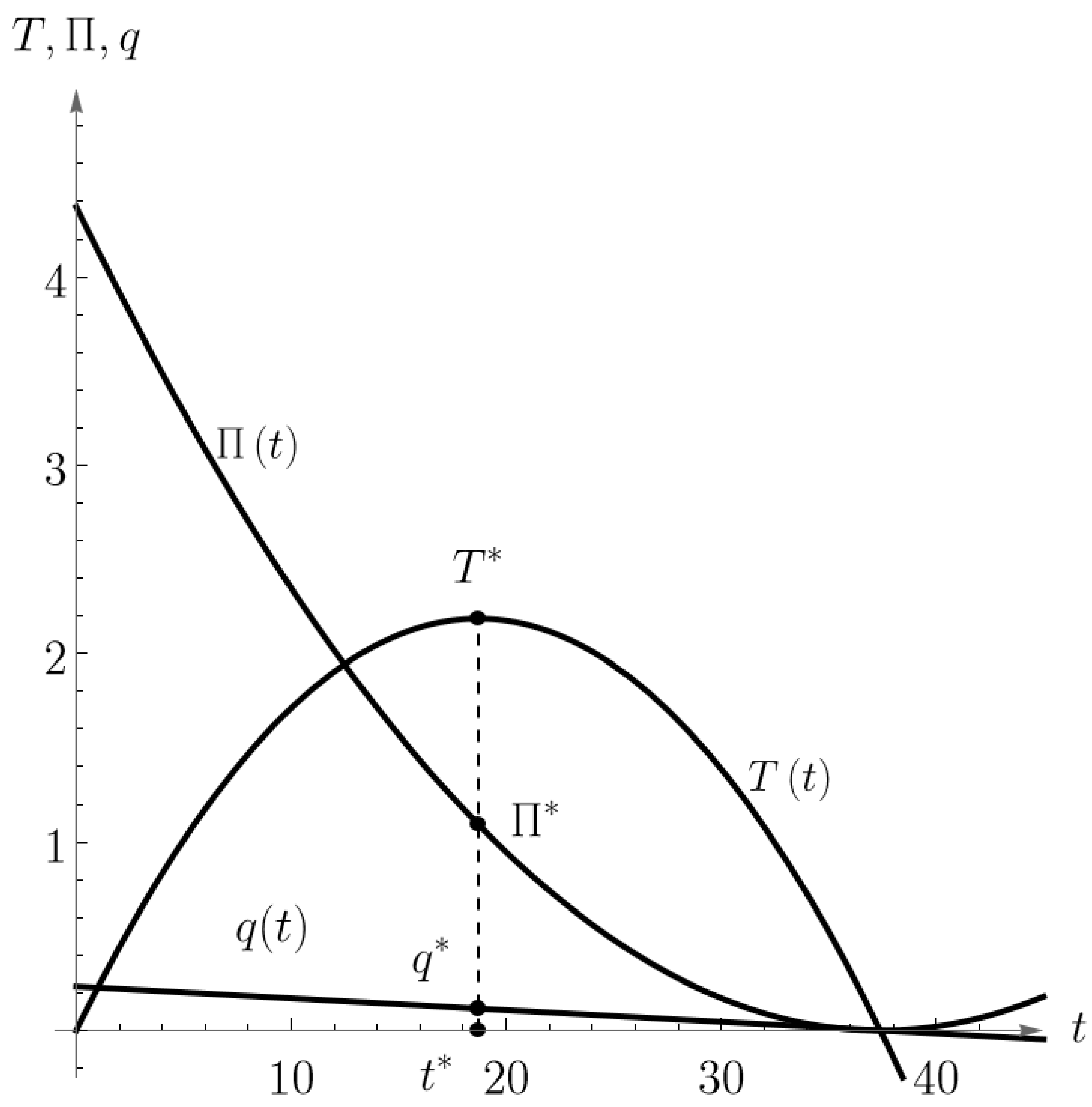
Figure 1 and
Figure 2 show 2D and 3D graphical representations of the optimal solution
and
(black points) and optimal value
and
of the bilevel problems (30) and (31) from Example 1. The pink-colored surface in
Figure 2 represents the leader’s
function. Purple-colored surface represents the follower’s
function. Green-colored vertical plane is the first-order condition
plane. If we express
from the first-order condition, we will obtain
and
functions just like in
Figure 1.
Furthermore, for constant returns to scale
, from the optimal output level
and (4) follows the optimal inputs (labor and capital) levels
and
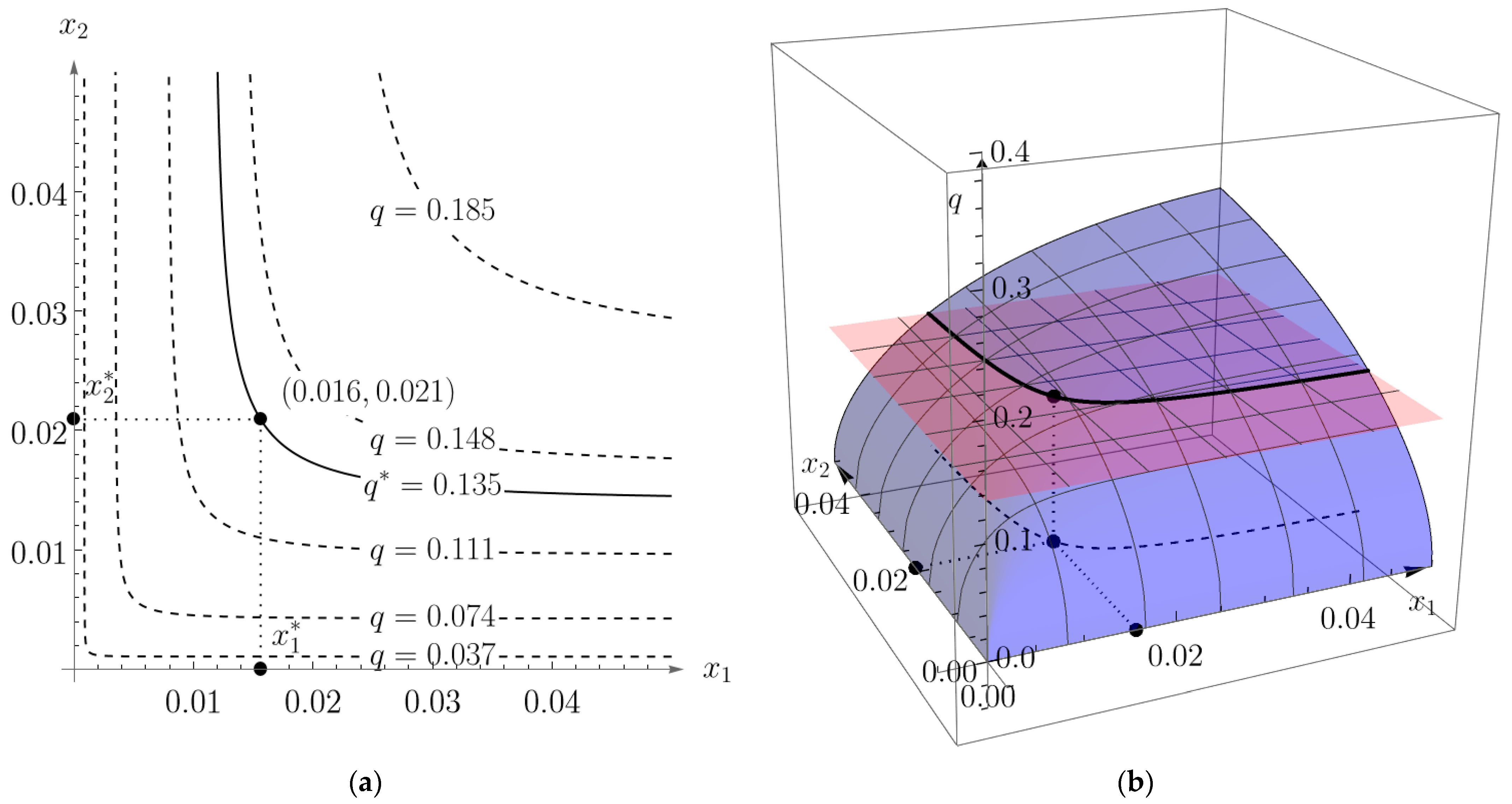
Graphical representations of the optimal capital and labor levels
and
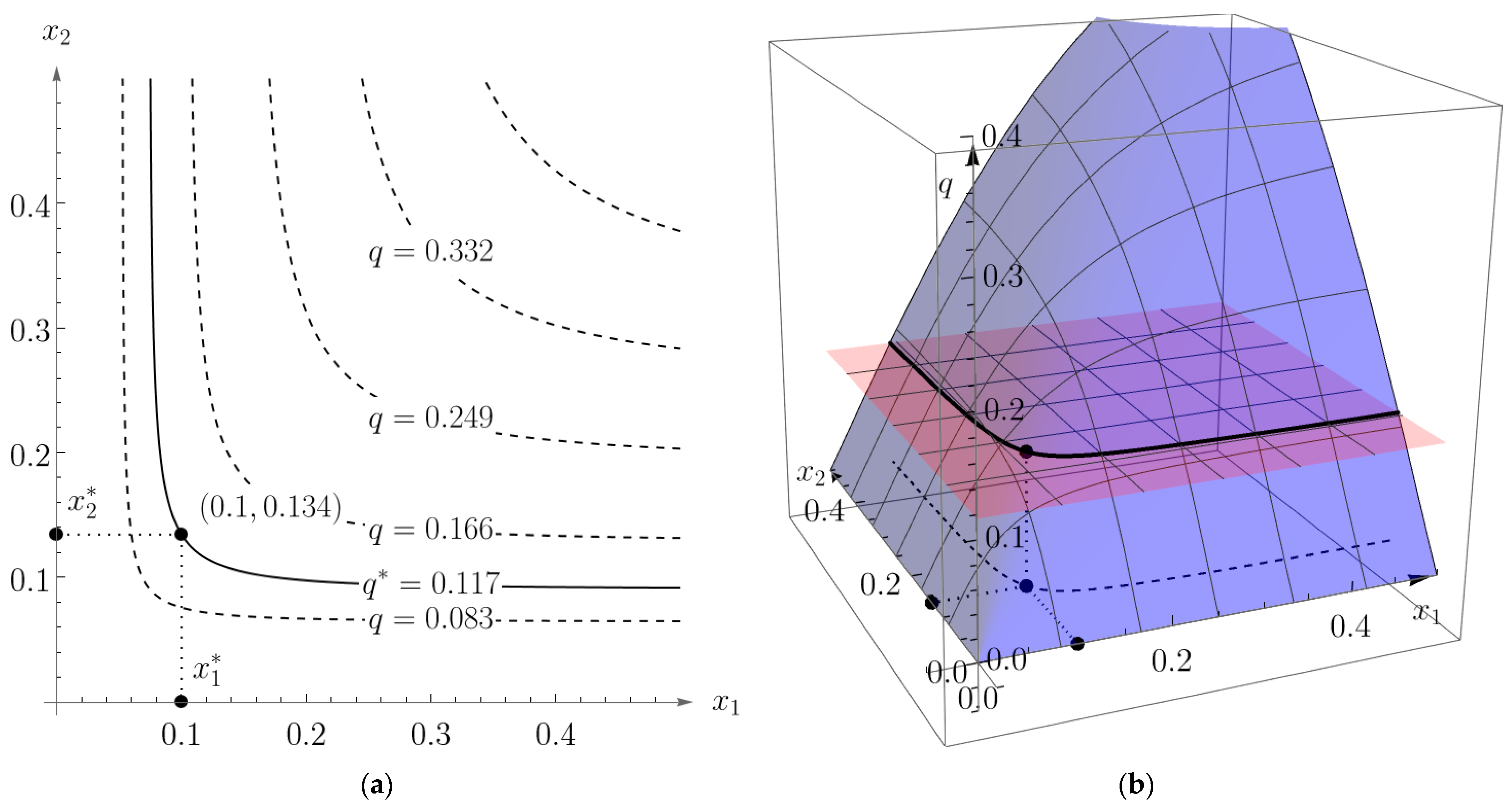
(black points) for the bilevel problems (29) and (30) are given in
Figure 3. The red horizontal plane in
Figure 3b is
plane and the blue surface is the CES production function
. A black solid curve represents the intersection of the red and blue surfaces. The black dotted curve is the projection of the intersection to
plane.
Figure 3a shows the level curves of the CES production function.
Corollary 2 (Decreasing returns of scale,
).
For the decreasing returns of scale bilevel programming problems (9) and (10) becomesThe optimal solution to the problems (14) and (15) is given bywhere
and
are the optimal leader’s and follower’s decisions, respectively. The optimal leader’s tax is equal towhile the optimal follower’s profit and input levels are, respectively, equal to Proof. For
Equation (13) becomes
which implies
Note that (33) implies the following condition:
Furthermore, since
the follower’s profit function is concave overall its domain in
q and the maximum profit is achieved. By substituting (46) with (38) we have
It is easy to see that the maximum of the function (49) equals (42) and that it is obtained for (40). That is, the optimal leader’s tax is equal to (36) and it is achieved at level (40). Now, substituting (40) into (46) we obtain (41). Finally, by substituting (40) and (41) into (39), we obtain (43). Furthermore, for decreasing returns to scale , from (41) and (4) follows (44). Finally, from (40) and (41) it is easy to check that inequality holds, which verifies (12). This proves the corollary. □
Example 2. Decreasing returns of scale: .
Let us consider the example similar to Example 1, but with the degree of homogeneity of the CES production function set to instead of 1. The number of inputs is again , the input prices and , respectively, the coefficients of the demand function and , respectively, the allocation coefficients of the CES production function and , respectively, the scale of production and the substitution coefficient of the CES production function .
The production function (1) is given by
Note that according to (3) again has the same value .
Since for
problems (38) and (39), i.e., (9) and (10) can now be stated as the following bilevel programming problem:
The optimal solution and of the problems (52) and (53) are given by Formulas (40) and (41), i.e., , , while the optimal leader’s tax according to (42) is given by and the optimal follower’s profit according to Formula (43) is given by .
Although the optimal solution and the optimal values of the problems (52) and (53) are already given by Formulas (40) and (43), let us consider and solve the problems (52) and (53) following the steps from Corollary 2 and let us look at the graphical representation of the problem given in
Figure 4,
Figure 5 and
Figure 6.
First, we solve the follower’s problem (53) for a given but fixed tax amount
t. From the first-order conditions on (53)
we obtain the optimal output level
Furthermore, since , the follower’s profit function is concave overall with its domain in q and the maximum profit is achieved.
By substituting
into the leader’s optimization problem (52)
we obtain the following tax revenue function of only tax amount
:
The maximum of the leader’s tax revenue function is obtained for because . It is easy to see that and .
Furthermore, the optimal output level
Finally, by substituting
and
back into the follower’s profit function, we obtain the optimal follower’s profit
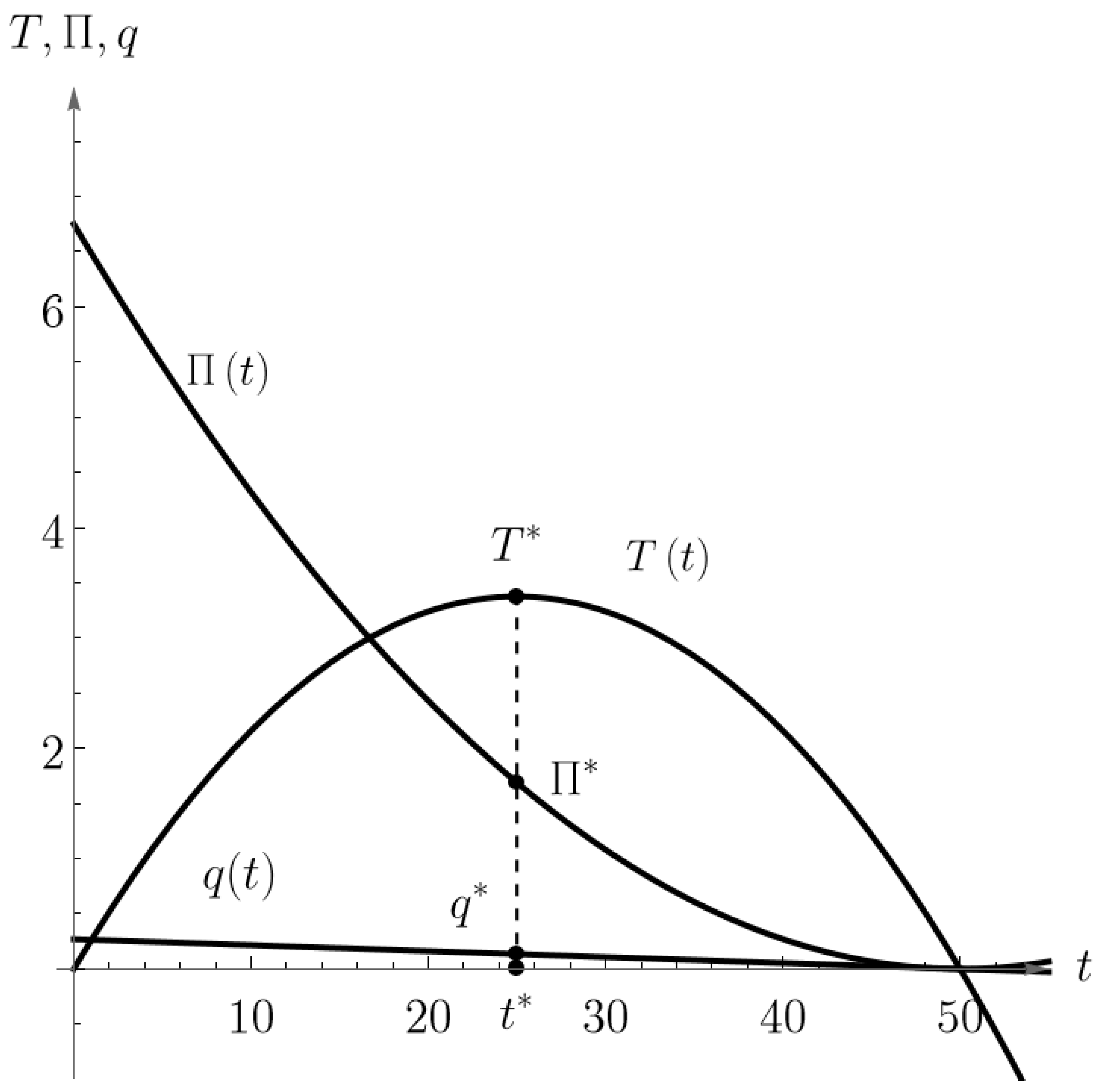
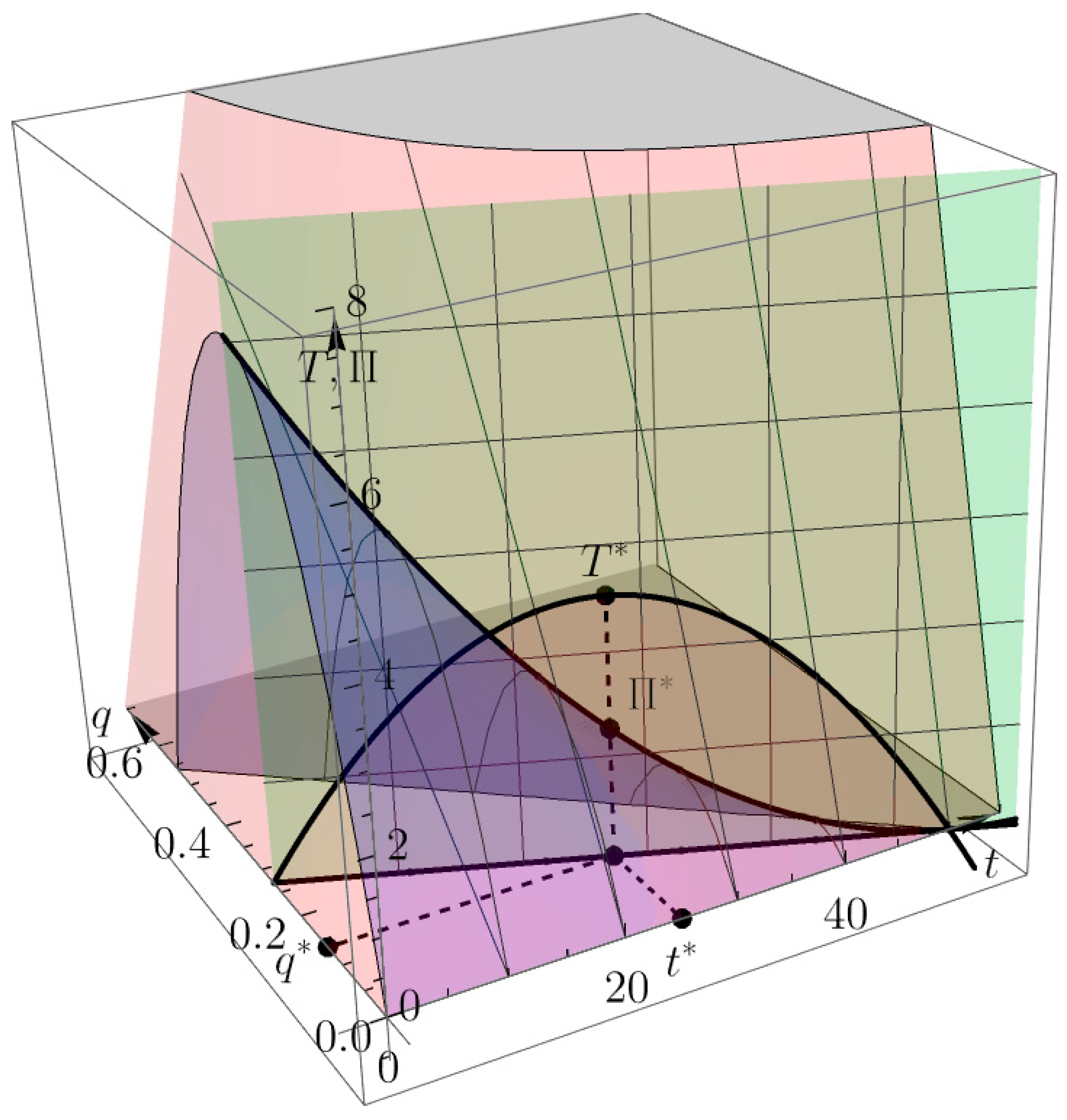
Figure 4 and
Figure 5 show 2D and 3D graphical representations of the optimal solution
and
(black points) and optimal value
and
of the bilevel problems (52) and(53) from Example 2. The pink-colored surface in
Figure 5 represents the leader’s
function. Purple-colored surface represents the follower’s
function. The green-colored vertical plane is the first-order condition
plane. If we express
from the first-order condition, we will obtain
and
functions just like in
Figure 4.
Furthermore, for decreasing returns to scale
, from the optimal output level
and (4) follows the optimal inputs (labor and capital) levels
and
Graphical representations of the optimal capital and labor levels
and
(black points) for the bilevel problems (52) and (53) are given in
Figure 6. The red horizontal plane in
Figure 6b is
plane and the blue surface is the CES production function
. Black solid curve represents the intersection of the red and blue surfaces. The black dotted curve is the projection of the intersection to
plane.
Figure 6a shows level curves of the CES production function.
According to [
22], when the follower operates as a perfect competitor, attaining maximum profit becomes unfeasible for increasing returns to scale, i.e., for
. However, within our models (9) and (10), given that the follower assumes a monopolistic role with the linear demand (5), the solution of the bilevel programming problems (9) and (10) is attainable for specific numerical parameter values within the model. We will illustrate this scenario with the following example.
Example 3. Increasing returns to scale: .
Let us consider the example with the degree of homogeneity of the CES production function set to , instead of to 1 or 0.5 as in the Examples 1 and 2. Let the number of inputs be . Let the input prices be and , respectively, let the coefficients of the demand function be and , respectively, and let the allocation coefficients of the CES production function be and , respectively. Furthermore, let the scale of production be and let the substitution coefficient of the CES production function be .
The production function (1) is given by
Note that according to (3) again has the same value .
Since for
Problems (9) and (10) can now be stated as the following bilevel programming problem:
First, we solve the follower’s problem (64) for a given but fixed tax amount
. From the first-order conditions on (64)
we should obtain the optimal output level
. Note that Equation (65) cannot be solved for
explicitly. Solving the problems (63) and (64) numerically, we obtain the optimal solution
and
with
. Note that
so
and
really maximize the follower’s problem (64).
Note that (6) implies . To solve the problems (63) and (64) numerically, one can generate values for t between 0 and 80 with step 0.001, for example, and then solve the first-order condition (65) for q. For obtained pairs (t,q) condition should be checked in order to ensure the maximization point for the follower’s problem (64). Finally, across all pairs (t,q), find the pair (t*,q*) that maximizes the leader’s function .
Note also that the bilevel programming problems (63) and (64) cannot be solved directly just by placing the model into some application. It is not easy to solve it even if the follower’s problem is replaced with first-order conditions (65).
Finally, by substituting
and
back into the follower’s profit function, we get the optimal follower’s profit
Furthermore, for increasing returns to scale
, from the optimal output level
and (4) follows the optimal inputs (labor and capital) levels
3.2. Some Sensitivity Analysis Remarks
In this subsection, we analyze how optimal solutions obtained in previously presented examples change when the price of the product received by the producer
changes. Let us recall from Equation (5) that
has a form
where
and
are coefficients of the demand function and
is the tax amount per unit product. Obviously, from (69), we can see that for fixed
and
as a function of a parameter
is linearly increasing, i.e.,
is increasing. Similarly,
is decreasing.
In the case of constant returns of scale where , from Corollary 1. we see that the change in parameter affects all optimal values (16) and (19), while the change in has an impact on (17) and (19) only. Precisely, from (16) and (19) we can see that if increases, the optimal leader’s (i.e., government’s) decision increases, the optimal follower’s (i.e., monopolist’s) decision increases, optimal government’s tax increases, and optimal monopolist’s profit increases, respectively. Similarly, if the parameter increases, then the optimal government’s decision remains the same, the optimal monopolist’s decision decreases, the optimal government’s tax decreases and the optimal monopolist’s profit decreases, respectively.
In the case of decreasing returns of scale where , from Corollary 2. we see that the change in parameter affects all optimal values (40) and (43), while the change in has an impact on (41) and (43) only. Precisely, from (40) and (43) we can see that if increases, the optimal government’s decision increases, the optimal monopolist’s decision increases, the optimal government’s tax increases, and the optimal monopolist’s profit increases, respectively. Similarly, if the parameter increases, then the optimal government’s decision remains the same, the optimal monopolist’s decision decreases, the optimal government’s tax decreases and the optimal monopolist’s profit decreases, respectively.
Closed-form expressions for optimal values (16), (19), (40), and (43) enable us to calculate precise percent changes in all of these values for a given change in parameters
and
.
Table 2 shows these calculations, where we assume increments in parameters
and
for
and
, respectively.
Data in
Table 2 are easily calculated from Corollary 1 and 2. As the final remark in this subsection, it is interesting to note that, both in the case of the constant returns to scale (
) as in the case of decreasing returns to scale (for
), the optimal government’s tax is twice as great as the optimal monopolist’s profit. Indeed, from Corollary 1 and Corollary 2, we have
