Abstract
Transfer learning (TL) has been employed in electroencephalogram (EEG)-based brain–computer interfaces (BCIs) to enhance performance for cross-session and cross-subject EEG classification. However, domain shifts coupled with a low signal-to-noise ratio between EEG recordings have been demonstrated to contribute to significant variations in EEG neural dynamics from session to session and subject to subject. Critical factors—such as mental fatigue, concentration, and physiological and non-physiological artifacts—can constitute the immense domain shifts seen between EEG recordings, leading to massive inter-subject variations. Consequently, such variations increase the distribution shifts across the source and target domains, in turn weakening the discriminative knowledge of classes and resulting in poor cross-subject transfer performance. In this paper, domain adaptation algorithms, including two machine learning (ML) algorithms, are contrasted based on the single-source-to-single-target (STS) and multi-source-to-single-target (MTS) transfer paradigms, mainly to mitigate the challenge of immense inter-subject variations in EEG neural dynamics that lead to poor classification performance. Afterward, we evaluate the effect of the STS and MTS transfer paradigms on cross-subject transfer performance utilizing three EEG datasets. In this case, to evaluate the effect of STS and MTS transfer schemes on classification performance, domain adaptation algorithms (DAA)—including ML algorithms implemented through a traditional BCI—are compared, namely, manifold embedded knowledge transfer (MEKT), multi-source manifold feature transfer learning (MMFT), k-nearest neighbor (K-NN), and Naïve Bayes (NB). The experimental results illustrated that compared to traditional ML methods, DAA can significantly reduce immense variations in EEG characteristics, in turn resulting in superior cross-subject transfer performance. Notably, superior classification accuracies (CAs) were noted when MMFT was applied, with mean CAs of 89% and 83% recorded, while MEKT recorded mean CAs of 87% and 76% under the STS and MTS transfer paradigms, respectively.
Keywords:
brain–computer interface; BCI; electroencephalogram; EEG; domain adaptation; inter-subject variation; transfer learning; single-source to single-target; STS; multi-source to single-target; MTS MSC:
68T07
1. Introduction
Brain–computer interfaces (BCIs) introduce a direct communication link that makes it possible to utilize neural activities of the brain to control external devices. These neural activities are extracted from the brain in the form of EEG signals and transformed into computer-readable commands used to control electrical devices. BCIs make use of several significant components to transform and translate EEG signals into control commands or the user’s intent. To achieve this goal, raw EEG signals are first pre-processed, mainly to eradicate artifactual interference through either filtering or signal decomposition techniques [1]. Artifact-free signals are then used to acquire relevant signal features from both the time and frequency domains and, subsequently, redundant features are rejected using feature selection techniques—highly useful for the selection of relevant feature subsets utilized for feature classification [2]. Afterward, the selected feature subsets, from a pool of both time and frequency domain features, are in turn used as input parameters to machine learning algorithms for the classification of the user’s intent [3]. In recent years, many researchers have introduced numerous experimentation paradigms in the form of steady-state visual evoked potentials (SSVEPs), including various algorithms that have been developed to enhance prediction rates in BCIs [4]. However, EEG signals are non-linear, continuous, and change over time and, as a result, neural dynamic variations across sessions and subjects exist [5], having a severe negative impact on the classification performance for both cross-session and cross-subject predictions in BCIs. In this case, such significant variations in neural characteristics can be attributed to domain shifts between the EEG recordings, leading to poor performance.
The literature [6] has illustrated that a significant challenge in MI-BCIs is the complexity of predicting neural activities between subjects that possess immense individual differences in EEG characteristics. Hence, a transfer data learning network (TDLNet) was proposed to mitigate the existing challenge of inter-session and inter-subject variability with more accurate intention prediction. The proposed TDLNet consisted of three components utilized to obtain the cross-subject intention recognition for multi-class upper-limb MI: The first component, in the form of the transfer data module, was employed to process cross-subject EEG data and fuse cross-subject channel features through two one-dimensional convolutions [6]. This was followed by an inception module that applied multiple parallel branches to obtain multi-scale time information from input feature maps. Lastly, a residual attention mechanism module (RAMM) allocated attention weights to various EEG signal channels for various MI tasks, focusing on the most relevant brain signals to improve the accuracy of the BCI decoding. Consequently, the highest prediction rate of 65% was recorded for a six-class cross-subject classification scenario.
Ref. [7] adopted cross-session and cross-subject strategies to evaluate the effectiveness of the proposed multi-source associate domain adaptation (DA) network for emotion recognition. Therefore, only domain-specific and invariant features were considered when the multi-source associate DA network was employed to address the disadvantages of EEG, which include low signal-to-noise ratio and non-stationary properties contributing to the large variation in EEG characteristics across subjects. The proposed integrated network model, consisting of shared subnets, achieved this goal by adapting the marginal distribution of different domains and employing conditional distribution while utilizing the maximum mean discrepancy and association reinforcement methods [7]. A multi-source associate DA network yielded remarkable performance for the cross-session scenario; however, a massive decrease in CA was observed for the cross-subject classification scenario, with average CAs of 65.59% and 59.29% captured for both the DEAP and SEED-IV datasets, respectively. Ref. [8] further illustrated that the performance of MI-based BCIs is massively affected by immense inter-subject variations, including the inherent non-stationarity of captured EEG signals. Subsequently, to mitigate the existing limitations, a novel logistic regression with tangent-space-based transfer learning (LR-TSTL) was utilized for the motor imagery [8]; in this case, an average CA of 78.95% was captured for within-subject classification scenarios, while an average CA of 81.75% was captured for cross-subject scenarios.
In ref. [9], a cross-scale transformer and triple-view-attention-based domain-rectified transfer learning (CST-TVA-DRTL) framework was proposed to mitigate the challenge of massive variations in EEG characteristics, mainly to improve cross-subject transfer performance. Therefore, to achieve the above-mentioned objective, the proposed CST-TVA-DRTL acquires transferable cross-subject invariant representations and utilizes domain-specific representation to rectify the domain-invariant representation. However, a decline in the prediction rate was observed when CST-TVA-DRTL was applied to 10 subjects from the PhysioNet dataset, with the highest CA of 73% recorded.
The impact of cross-subject EEG classification on the intention detection rate (IDR) was further investigated under one-to-one and multi-to-one transfer paradigms in [10]. In this case, an evolutionary programming neural network ensemble (EPNNE) technique was proposed for emotion recognition, mainly to address the challenges of significant individual differences and the non-stationary characteristics of EEG—including the complexity and variability of emotions. The proposed EPNNE was evaluated on four publicly available datasets, recording a superior average CA of 81% for the one-to-one transfer paradigm and an average CA of 89% for the multi-to-one transfer paradigm for cross-subject emotion recognition [10]. The literature further validated that the inherent non-stationarity of EEG signals and the immense inter-subject variations in EEG characteristics—emanating from domain shifts between the EEG recordings—remains a significant challenge in the EEG-based BCIs studied.
In this paper, the effect of domain shifts between the EEG recordings that lead to poor cross-subject transfer performance is investigated, mainly to address the challenge of significant variations in EEG characteristics from subject to subject. Subsequently, domain adaptation algorithms—including ML algorithms implemented through a traditional BCI—are presented and contrasted to determine the impact of the immense inter-subject variations in EEG characteristics on cross-subject transfer performance. Therefore, to facilitate this investigation, both domain adaptation algorithms (MMFT and MEKT) are examined under single-source-to-single-target (STS) and multi-source-to-single-target (MTS) transfer learning paradigms. Notably, to carry out a fair contrast between the domain adaptation algorithms and ML algorithms, similar transfer learning paradigms (STS and STM) are emulated for both NB and K-NN classifiers. The contributions of this study are summarized as follows:
- Investigate the effect of domain shifts between EEG recordings that contribute to significant variations in EEG characteristics from subject to subject;
- Assess the performance of domain adaptation methods—including ML algorithms implemented through a traditional BCI—under STS and MTS transfer learning paradigms based on a cross-subject EEG classification scenario;
- Conduct an extensive comparative performance analysis among MMFT, MEKT, K-NN, and NB. The results acquired from the experiments illustrated that domain adaptation algorithms yield superior performance under both the STS and MTS transfer learning paradigms compared to classical ML algorithms for cross-subject EEG classification.
The rest of this paper is structured as follows: Section 2 reviews related work on domain adaptation algorithms and traditional BCI frameworks for cross-subject classification. Section 3 presents the materials and methods. Section 4 describes the implementation of DAA and ML algorithms under STS, and MTS transfer paradigm. Section 5 presents the experimental results for both the STS and MTS transfer learning paradigms. Discussion and analysis of results is presented in Section 6. Finally, Section 7 draws the conclusions.
2. Related Work
Over the past decade, non-invasive EEG-based BCIs have been researched with the intention to enhance classification performance. Hence, different EEG signal acquisition paradigms, including various algorithms, have been developed to improve BCI performance with more accurate intention detection [11]. Signal acquisition paradigms, including MI, SSVEP, and P300, have been introduced while various signal processing techniques such as signal filtering and decomposition, feature extraction, and selection—including feature classification algorithms—have also been developed to improve performance [12,13,14,15]. In this case, a lot of progress toward enhancing BCI performance has been made for within-subject classification. Consequently, immense inter-subject variations emanating from domain shifts between EEG recordings still remain the most significant challenge for BCIs [16]. Domain shifts between EEG recordings can be attributed to some critical factors such as concentration, mental fatigue, and physiological and non-physiological artifacts leading to immense inter-subject variations [13,17]. Such individual differences are a major challenge in cross-subject EEG classification; hence, training a model from previous subjects’ EEG signals is not directly applicable to a new subject, mainly because different subjects have different neural responses to the same stimulus [18,19]. In ref. [20], an EEG-based BCI was presented to show evidence of the variabilities in EEG neural dynamics, whereby a pair-wise performance associativity technique was employed to investigate the impact of inter-session and inter-subject variability on performance. In this instance, employing a two-layer feed-forward neural network to train using features from a single subject or session while using features from another subject or session to predict proved to massively deteriorate the CA [20]. Jie et al. [9] illustrated that EEG classification performance can be compromised due to the limited representation learning ability of the model since existing deep learning methods consider discriminative multi-view spectral and dependencies of multi-scale temporal features, while most TL-based approaches commonly ignore individual-specific information and fail to acquire transferable cross-subject invariant representation. Hence, a domain-rectifier transfer learning (DRTL) framework was introduced to mitigate the above-mentioned limitations; however, applying DRTL on the physioNet dataset to acquire untransferable domain-specific and transferable domain-invariant representations and then rectifying the domain-invariant representation to adapt to the TD using domain-specific information resulted in a significant decrease in prediction rate [9]. In ref. [21], a deep transfer learning technique was extended to an EEG multi-subject training scenario to mitigate the inherent challenge of training CNNs using multiple subjects without reducing individual performance since CNNs cannot directly utilize samples from multiple subjects’ EEG to improve model performance directly [21]. A multi-branch deep transfer network in the form of a separate-common-separate network (SCSN) was proposed, which is based on separating the network’s feature extractors for each subject. Applying SCSN yielded superior CA when employed on the BCI Competition IV-a-IIa dataset, while a massive decrease in CA was captured when employed on online recorded data.
Ref. [22] proposed a model-independent strategy for a cross-subject MI EEG-based BCI in the form of multi-direction transfer learning (MDTL), whereby MDTL was deployed on three deep learning models, namely ConvNet, ShallowConvNet, and EEGNet. Notably, a decrease in CA was observed when MDTL was deployed on EEGNet using the four-class BCI IV-a dataset, with a mean CA of 75% recorded [22]. When MDTL was deployed on ConvNet and ShallowConvNet, mean CAs of 80.86% and 81.95% were recorded.
These papers collectively contribute diverse approaches to EEG-based BCIs for cross-subject classification, each demonstrating promising results in mitigating various challenges.
3. Materials and Methods
This section gives a detailed description of the experimental paradigm used for three EEG datasets and the methods used to facilitate the investigation. In this case, two transfer learning paradigms, through which all algorithms are implemented for experimentation, are discussed. Furthermore, the acquisition of the recorded MI, SSVEP, and BCI Competition IV-a datasets [23] and a BCI framework—through which cross-subject classification is implemented using classical classification algorithms—is discussed. Additionally, the domain adaptation frameworks utilized to achieve the objective of this study are presented in this section.
3.1. EEG Signal Acquisition
3.1.1. Dataset IIa of BCI Competition IV-a
A publicly available database designed by experts in the field containing dataset IIa for BCI Competition IV was used for experimentation [24]. Thus, EEG signals were recorded from nine healthy subjects in the experiment while each subject performed four MI tasks, namely, left, right, up, and down. Therefore, twenty-two EEG channels or Ag/AgCI electrodes were employed to extract the neural activities of the brain in the form of MI tasks. A sampling rate of 250 Hz was used when raw EEG signals were recorded from the brain [25]. A 10–20 positioning system was used to position electrodes on the surface of the scalp, with each electrode 3.5 cm apart. In this instance, EEG signals were already pre-filtered to minimize the effect of artifacts, whereby a 50 Hz notch and a band-pass filter at a cut-off frequency between 0.5 and 100 Hz were applied to MI signals from the BCI Competition IV-a dataset [1,26]. At the beginning of a trial experiment, participants were seated facing a monitor. A fixed cross was projected onto the monitor to indicate the beginning of a trial at t = 0 s. A beeping sound, which lasted for two seconds and is denoted by t = 2 s, was the external stimulus to signify the start of a trial. Then, followed by visual cues projected on the monitor for t = 1.25 s, each visual cue signified an MI task denoted by an arrow pointing to a direction equivalent to the MI task. Afterward, from t = 3.25 s to t = 6 s, the experiment participants were instructed to perform four imagined movements, as depicted in Figure 1 [25].
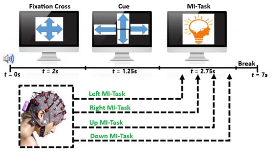
Figure 1.
Timing of the recording paradigm for dataset IIa of BCI Competition IV.
3.1.2. Recorded MI and SSVEP Datasets
A Simulink model was interfaced with a gtec EEG recording system via MATLAB R2015a to enable the acquisition of the recorded MI and the SSMVEP datasets, as depicted in Figure 2. The EEG recording system consisted of a gNautilus headset and a gNautilus base station, which established wireless communication between the two components. The gNautilus headset included 16 electrodes and a transmission module that made it possible to transmit raw EEG signals to the Simulink model. When the model began executing, the gNautilus block received EEG data from the gNautilus headset via the gNautilus base station; meanwhile, the logic control block was executing a MATLAB function that notified the subject through a beeping sound to start performing each of the four EEG classes for 300 s, respectively, with the aid of the real-time clock block. Moreover, the prepare_for_online block was used to filter raw data, transforming the filtered data to ICs; then, it extracted signal features from ICs, at the same time saving both the raw data and extracted signal features for offline BCI analysis, as illustrated in Figure 2. The online_BCI_control block was not used.
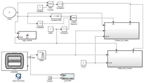
Figure 2.
Simulink model for EEG data acquisition.
Figure 3 depicts the timing scheme of the experiment paradigm for the recorded MI dataset, acquired using a gtec EEG recording system consisting of 16 electrodes. EEG signals were recorded from 9 healthy experiment participants (8 males and 1 female; age: 25–35 years old) in a confined laboratory. Subsequently, a 10–20 positioning system positioned all sixteen EEG channels on the surface of the scalp, while a sampling rate of 250 Hz was applied during the acquisition of the MI signals [27]. Afterward, a 50-hertz notch filter, a band-pass filter at a cut-off frequency between 0.5 and 60 Hz, and a common average reference (CAR) filter were applied to the recorded MI to mitigate the effect of interference during EEG recording [1,26]. In this case, the recorded MI dataset came from nine healthy experiment participants performing four imagined movements, namely, left, right, up, and down [28]. At the start of a trial experiment, participants were instructed to perform four EEG classes corresponding to four imagined movements. Each MI task was performed for 300 s, while participants were seated facing a monitor. Four arrows corresponding to each MI task were projected on the screen, accompanied by a beeping sound to signify to the experiment participant to start performing imagined movements, as depicted in Figure 3.
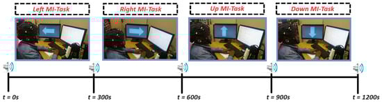
Figure 3.
Timing of the recording paradigm for captured MI datasets [29].
For our own recorded SSMVEP dataset, a similar experimental setup to the recording of the MI dataset was used. In a similar manner, EEG signals were recorded in a confined laboratory from 9 healthy experiment participants (8 males and 1 female; age: 25–35 years old). A 50-hertz notch filter, a band-pass filter at a cut-off frequency between 0.5 and 60 Hz, and a common average reference (CAR) filter were also applied to the recorded SSMVEP signals [1,26]. When the experiment began, four cups consisting of four flashing LEDs were used as visual stimuli. The four LEDs represented four frequencies—29 Hz, 17 Hz, 21 Hz, and 13.3 Hz—corresponding to four EEG classes. The frequencies were tagged on the flashing LEDs attached on the cups, representing four SSVEP classes, namely, left, right, up, and down [30,31]. When the trial began, a beeping sound indicated that the participant must concentrate on one single flashing cup at a time, and each SSVEP class lasted for 300 s, as depicted in Figure 4 [32].
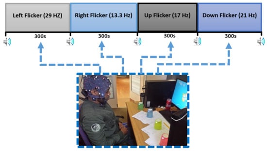
Figure 4.
Timing of the recording paradigm for the captured SSVEP datasets.
3.2. Domain Adaptation Algorithms Based on Cross-Subject EEG Classification
In this section, two domain adaptation algorithms are introduced—namely, manifold embedded knowledge transfer (MEKT) [33] and multi-source manifold feature transfer (MMFT) [34]. Notably, both domain adaptation algorithms are implemented based on cross-subject EEG classification but can be further extended to address the challenge of significant variations in EEG characteristics with a focus on STS and MTS transfer learning paradigms.
3.2.1. Manifold Embedded Knowledge Transfer Framework (MEKT)
This section introduces a transfer learning framework to evaluate the impact of cross-subject classification on prediction rate. In this case, the MEKT framework is implemented under two transfer learning approaches, namely STS and MTS. The framework utilizes features acquired from either an individual subject or numerous subjects (source domains) to enhance the prediction rate of another individual subject (target domain). The first step is to ensure proper transferability of the knowledge from various source domains; then, in the second step, the MEKT framework minimizes the marginal probability distribution shift by closely aligning the centroid of the covariance matrices.
Therefore, alignment of the covariance matrix centroid serves as a pre-processing phase employed to lower the marginal probability distribution shift of different domains, mainly to enable the transferability of features from different domains. Consequently, Equation (1) is used to align covariance matrices from source domains, where represents the aligned covariance matrices acquired from either an individual or numerous subjects (source domain), while represents the covariance matrices acquired from a different individual subject (target domain) and can also be generated in a similar manner. In this case, the number of covariance matrices contained in the source domain is denoted by , while represents the Riemannian mean of matrices [33], used as the reference matrix denoted by to minimize inter-subject and inter-session variations. Moreover, the covariance matrix in the source domain is denoted by .
Equations (2) and (3) are used to generate tangent space feature vectors through mapping of all covariance matrices, once the marginal probability distribution shift of various domains are minimized after the alignment.
In this case, Equations (4) and (5) represent the tangent space features extracted from aligned covariance matrices in the source and target domains, respectively. Once tangent space features are extracted, the classifier is trained using , with and being the features and class labels, respectively, from the source domains. Moreover, to acquire pseudo labels for the target domain, the classifier is tested using , whereby represents target domain tangent space features, and is the target domain projected matrices. In this case, both and represent projected matrices used to map and to lower dimensional matrices.
Furthermore, to measure performance in this case, Equation (6) representing the balance classification accuracy, denoted by , is used, where represents the class; the number of source domain class labels is denoted by ; represents the number of true positives; and the number of samples contained within a class is denoted by [33]. The MEKT framework utilizes a shrinkage linear discriminant analysis (sLDA) classifier, which is based on the optimal shrinkage estimate [35]. The classifier makes use of three inputs to predict target domain labels denoted by . In this case, the first input represents source domain features denoted by ; target domain features are denoted by ; and lastly, the source domain labels are denoted by .
3.2.2. Multi-Source Manifold Feature Transfer Learning (MMFT)
In ref. [34], an MMFT algorithm was employed based on a less-complex classification problem, namely, a two-class problem, to mitigate the effects of subject-to-subject and session-to-session variabilities in electroencephalogram neural characteristics. When the MMFT framework is implemented, the DMA is first employed—through which the objective function, depicted in Equation (7), similarly disseminates all domains between the SPD manifold.
where the linear transformations are denoted by both A and B; the distribution means of the SDs and TDs are denoted by and respectively; and the covariance matrix deviations for the SDs and TDs are denoted as and respectively. As depicted in Equations (8) and (9), the optimal solution of , including two feasible solutions, was achieved by reducing the objective function derived from Equation (7). Notably, from Equation (7) one finds if , then the objective function obtains the optimal solutions. In this way, the marginal probability distribution shift was reduced between the SDs and TDs, i.e., aligning the distribution means.
The linear transformations in Equation (8), denoted by A and B, were further applied for the distribution mean alignment to every domain’s Riemannian center.
Using Equation (9), the identity matrix consisting of proper dimensions is represented by ; represents the target domain distribution mean; and represents the source domain distribution mean aligned with the TD. Thus, Equations (10) and (11) compute the covariance matrices across both SDs and TDs once the distribution means are aligned.
where the -th trial of the EEG samples of the covariance matrix in the SD is denoted by ; the -th trial of the EEG samples of the covariance matrix in the TD is denoted by ; and the aligned covariance matrices of the SDs and TDs are denoted by and respectively. The next phase of the MMFT framework is the SPD manifold-tangent-space feature extraction using Equations (12) and (13).
Equations (12) and (13) extract the tangent space features, where and are numerical representations of trials contained in the SD and the TD, respectively, and the extracted tangent space features across the source and target domain are denoted by and . Therefore, Equations (14) and (15) represent the matrices of the extracted feature sets, with both and representing the tangent space features generated from both the source and target domains, respectively [33,34].
Feature learning via the Grassmann manifold (GFK) was employed in the third stage of MMFT. Here, the average stable features are identified using the GFK during the conversion process on the geodesics from SD to TD [36]. The GFK brings the deviations of all covariance matrices closer by minimizing the marginal probability distribution [34,37]. Therefore, Equation (16) was used to compute the feature learning, denoted by ; denotes the extracted tangent space feature; and represents the geodesic flow.
Equation (17) achieved the inner product of the transformed features.
where the geodesic flow is denoted by the tangent space features are denoted by ; and the newly learned Grassmann manifold is denoted by . Moreover, when is transformed to , represents the transformation. Hence, Equation (18) expresses the Grassmann manifold features obtained after the transformation.
The fourth stage of the MMFT framework uses the MMFT classifier. Training the prediction model of Equation (19) reduced the structural risk between SDs, while the conditional alignment was summarized [34].
With the diagonal label indicator matrix denoted by .
Equation (20) signifies the conditional distribution discrepancy of the prediction model denoted by . Therefore, represents conditional distribution alignment.
The classifier denoted by was computed using Equation (21), achieved by integrating both Equations (19) and (20). Both SD and TD samples are denoted by and , respectively [34].
When the representer theorem was applied, Equation (22) accepted an expansion, with representing the coefficient vector and the kernel generated through feature-mapping is denoted by . The kernel was used to estimate the original feature vector to a Hilbert space [34].
The structural risk minimization on the SD was computed using Equation (23), with the coefficient vector denoted as ; represents the frobenious norm; and represents the kernel matrix. The trace operation is denoted by , while represents the label matrix for both SD and TD [34].
Equation (24) was obtained by integrating the kernel with the representer theorem to further transform the conditional distribution alignment, whereby represents the maximum mean discrepancy [34].
Elements of the maximum mean discrepancy are computed using Equation (25), wherein and represent samples contained in Class C for both SD and TD.
Equation (26), denoted by , represents the objective function acquired by integrating Equations (23) and (25) to minimize the conditional probability distribution shift and the loss function.
The derivative denoted by helps to obtain the solution to the objective function, making use of Equation (27), with Equation (24) measuring the classifier after was achieved.
The last phase of MMFT is employed for quantified voting to transfer knowledge from various sources. The voting mechanism is used to combine the prediction information acquired from various domains, mainly for class labels for the TD. Thus, Equation (28) votes for the classification results of each classifier. The transfer of features between domains is dependent on the results acquired through the voting mechanism when the classifiers are examined [34]. Therefore, each classifier is implemented utilizing Equation (25) whenever each of the SDs is transferred.
Furthermore, to mitigate the effects of class imbalance due to label information in the source domain, a weighted MMFT (w-MMFT) algorithm is also explored to address the class imbalance, which occurs as a result of the source domain label information and tends to affect the structural-risk function used to train the MMFT classifier [34,38]. In this instance, the w-MMFT’s objective function is defined by Equation (29), with representing the weight matrix.
The solution to the objective function, represented by Equation (29), is defined by Equation (30). The weight matrix is denoted by and the maximum mean discrepancy matrix is denoted by [34]. The MMFT framework was only evaluated on a less complex classification problem, namely, a two-class problem; the algorithm has not yet been evaluated on more complex prediction problems such as three-class or four-class problems.
3.3. Proposed Traditional BCI Framework Based on Cross-Subject Classification
Figure 5 gives a detailed overview of the proposed traditional EEG-based BCI pipeline through which ML algorithms are implemented under STS and MTS transfer paradigm, to evaluate the impact of significant variations in electroencephalogram dynamics contributing to poor prediction rate in BCI.
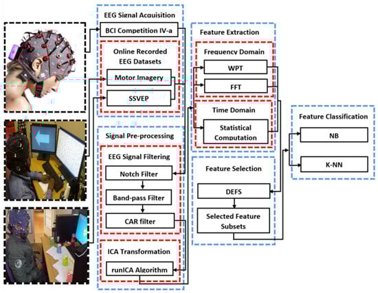
Figure 5.
Traditional BCI framework for K-NN and NB implementation.
3.3.1. EEG Signal Pre-Processing
Filtering of EEG Signals
First, a 50-hertz notch filter was applied to the BCI Competition dataset to eradicate the effects of line noise originating from electrodes positioned on the scalp. This was followed by a band-pass filter at a cut-off frequency between 0.5 Hz and 100 Hz to remove the effects of noise or various other non-physiological artifacts [25,39].
Notably, a band-pass filter at a cut-off frequency between 0.5 Hz and 60 Hz was applied on both gtec recorded EEG datasets to filter all non-physiological artifacts. Therefore, the Butterworth band-pass filter was computed per Equation (31), where represents angular frequency in radians per second; and denotes the filter order [40]. A 50-hertz notch filter was further employed to remove noise originating from EEG channels on the surface of the scalp [25,41].
EEG signals were further filtered via common average reference (CAR) to remove noise and to enhance signal-to-noise. Thereafter, Equation (32) was used to compute the CAR, with representing the reference; representing the potential across electrodes; and n depicting the number of EEG channels [42].
Decomposition of EEG Signals
The runICA algorithm was employed to remove the effects of physiological artifacts, including EOG, ECG, and EMG from the two recorded EEG datasets, together with dataset IIa of BCI Competition IV [1,41]. Hence, filtered EEG signals generated ICs, from which non-contaminated components are selected to mitigate the effects of both physiological and non-physiological artifacts [43]. Consequently, artifactual components are rejected, while clean components are reconstructed into mutually independent components or artifact-free ICs [44].
Thus, ICs were computed using Equation (33), with depicting the source signals; and depicting random noises contained within various observations. Furthermore, a vector of rows was denoted by , while a mixed matrix was denoted by A [1,45].
The signal sources separated utilizing ICA are given by Equation (34), whereby represents the separated signal sources, with each component depicting an estimate of an independent source signal to an indeterminacy of scale and order; W represents a reversible matrix; and a whitened matrix is denoted by V [45].
3.3.2. Extraction of EEG Signal Features
Three sets of signal features were extracted from the artifact-free reconstructed ICs once artifactual components were rejected; in this instance, wavelet, band-power, and statistical features were extracted. First, 255 wavelet features were extracted using wavelet packet transform (WPT)—which is an extension of discrete wavelet transform (DWT)—from the ICs [46]. Wavelet packet transform (WPT) was considered for feature extraction due to its ability to exhibit highly significant and informative low and high frequencies of EEG signals [46].
A Daubechies of order 4 (db4) was implemented through Equation (35), denoted by , which was used to compute WPT. Here, WPT first decomposed ICs into a wavelet packet tree consisting of seven decomposition levels [47,48]. The wavelet packet tree consisted of detail and approximation coefficients at each decomposition level. The detail coefficients were generated from decomposed ICs by employing a wavelet function denoted by , while approximation coefficients were generated from decomposed ICs by employing the scaling function denoted by . In addition, the numbers of samples obtained from source signals were denoted by ; the number of the scales was denoted by and , representing the subband index of each scale; the detail-level expansion coefficients were denoted by ; and the coarse-level expansion coefficients were denoted by .
Furthermore, the dilated and translated versions of the wavelet function were represented by , while the translation and dilated versions of the scaling function were denoted by [49,50]. Consequently, wavelet coefficients were further decomposed into multiple windows to generate wavelet features by employing the sliding-window technique on a wavelet packet tree. A sampling frequency of 750, which is equivalent to 3 s, was set as the window size; every 3 s, a window was shifted by 750 samples until the end of the signal. Wavelet features were extracted from the wavelet coefficients in each decomposition level of a wavelet packet tree: a total of 255 wavelet features were extracted.
Second, fast Fourier transform (FFT) was employed to extract frequency domain features in the form of band-power features from reconstructed artifact-free ICs. Therefore, band-power features depicted by seven frequency bands—namely, mu, alpha, theta, delta, gamma, beta, and central beta—were extracted [42,51,52]. FFT was further employed to generate ten statistical features consisting of both time and frequency domain features. Hence, seven time-domain features (spectral entropy, kurtosis, skewness, mean absolute deviation, standard deviation, median, and mean) were extracted; meanwhile, three frequency domain features in the form of dominant frequency characteristics (maximum ratio, maximum frequency, and maximum value) were extracted. In this case, FFT was computed using Equation (36) denoted by , with sampled values denoted by ; the domain vector indices denoted by i; and representing the size of a signal domain [42,51].
3.3.3. Selection of EEG Signal Features
Feature selection was employed to address the challenge of dimensionality and the presence of redundant features from extracted feature sets. Hence, a differential evolution-based channel and a feature-selection (DEFS) algorithm were employed to identify highly informative features with high predictive power [2]. In selecting highly predictive features, the DEFS engages two techniques, namely, repair mechanism and differential evolution (DE) optimization [2].
Therefore, the number of iterations across each of the selected feature populations is controlled by employing a scale factor denoted by , acquired through Equation (37), while the constant lower than 1 is denoted by [2].
The population members could oscillate within bounds without crossing the optimal solutions, as in Equation (38). Here, the number of features is denoted by NF [2].
Furthermore, to avoid repetition of the selected features from the same vector of features, the distribution factor denoted by is employed and computed using Equation (39), with representing the overall number of features. Thus, a1 represents the appropriately identified constant that displays the importance of features in PD. Features possessing lower fitness when evaluated against the average fitness of the whole population are denoted by . The desired number of features to be selected is denoted by , while features possessing higher fitness when evaluated against the average fitness of the whole population are denoted by [2].
Notably, evaluation of the previous iteration against the current iteration was carried out per Equation (40) to identify subsets that have produced significant improvements and that grant superior weights to enhance features to be applied in the next iteration, with the distribution factor denoted by [2].
Equation (41) determined the number of times a specific feature was used within each iteration based on the updated distribution factor [2].
Subsequently, when the DEFS algorithm was employed to select relevant feature subsets, several parameters were put in place, with 80 set as the number of desired features denoted by DNF, 150 set as the population size denoted by PSIZE, and 1000 set as the number of generations denoted by GEN—at the same time being the terminating condition for the algorithm [2].
3.3.4. Classification of EEG Signal Features
In this section, a comparative performance analysis was carried out between transfer mapping and two classical machine learning (NB and K-NN) algorithms to determine whether neural activities acquired from different sources can enhance the prediction rate of either a single session or a subject.
K-Nearest Neighbor (K-NN)
K-nearest neighbor (K-NN), a supervised machine learning algorithm, applied the training set to identify k samples possessing the same independent variables. Hence, the classification algorithm was applied on both the recorded MI and SSMVEP datasets, including the BCI Competition IV dataset, to predict four EEG classes [49,53].
The K-NN measures the distance between instances in order to acquire various sets of k-nearest neighbors. Therefore, to compute the Euclidean distance, Equation (42) denoted by was applied. Moreover, x and y represent the feature spaces for two vectors; and and yi represent the coordinates of the two vectors in the feature space [2,54].
4. Implementation of Domain Adaptation and ML Algorithms Based on STS, MTS Transfer Paradigm
In this study, the effect of the single-source-to-single-target transfer learning paradigm on the prediction rate is first investigated with an emphasis on cross-subject classification. Subsequently, MEKT and MMFT are adopted, extended to a multi-class classification scenario, modified, and implemented according to the STS transfer learning paradigm experiment. The introduced domain adaptation algorithms are then contrasted with two classical ML algorithms (K-NN and NB)—mainly to determine the impact of domain shifts between EEG recordings on classification performance—and at the same time to mitigate the challenge of significant variations in EEG characteristics that lead to poor performance from subject to subject. To facilitate the investigation, three EEG datasets (BCI Competition IV-a dataset; the recorded MI and SSVEP datasets) are used for experimentation.
Notably, under the STS transfer learning paradigm, multi-class samples () including the corresponding class labels () from nine domains (subjects) are used as input parameters to both the MEKT and MMFT frameworks. In this case, when both domain adaptation algorithms are employed under the STS transfer learning approach, a single subject is assigned as the SD, denoted by (), and the corresponding class label, denoted by (), while another subject is assigned as the TD, depicted in Figure 6. Therefore, both algorithms iterate through the remaining eight subjects, assigning a single subject denoted by () as TD in each iteration and the predicted labels for the associated TD denoted by (). The number of iterations () is dependent on the number of subjects and each of the remaining subjects takes a turn as the TD in each iteration. Furthermore, to establish a fair contrast between MEKT, MMFT, and ML algorithms, a similar STS transfer learning paradigm experiment was emulated for both K-NN and NB classifiers. Therefore, to emulate a similar STS transfer learning approach using both classical ML algorithms, 80 optimal feature subsets selected from 271 extracted features from a single subject (SD) are utilized to first train the classifiers, while another 80 selected feature subsets from a different individual subject (TD) are utilized to predict for both the K-NN and NB classifiers.
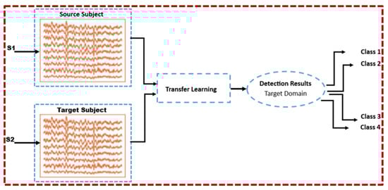
Figure 6.
Single-source-to-single-target transfer paradigm (STS).
Second, the impact of the multi-source-to-single-target TL paradigm on the prediction rate was further investigated using the same EEG datasets (BCI Competition IV-a dataset; the recorded MI and SSVEP datasets) for experimentation. To further facilitate the investigation, a contrast between MEKT and MMFT, including K-NN and NB, is carried out with an emphasis on cross-subject classification, mainly to determine the effect of domain shifts contributing to massive inter-subject variations in EEG neural dynamics on performance. Notably, similar parameters as in the STS TL paradigm are put in place when MEKT and MMFT frameworks are implemented based on the MTS transfer learning paradigm, as illustrated in Figure 7. Hence, both domain adaptation algorithms first receive samples from multiple sources together with the corresponding class labels. However, both MEKT and MMFT iterate through subjects, assigning an individual subject as a TD denoted by (), while the remaining subjects are assigned as SD denoted by (), including the corresponding class label denoted by (). Moreover, in each iteration, an individual subject is assigned as the TD to predict the target domain label denoted by () using SD samples. Furthermore, to reproduce a similar MTS transfer learning paradigm experiment for both K-NN and NB—mainly to carry out a fair contrast between domain adaptation and ML algorithms—80 optimal feature subsets selected from 271 extracted features from an individual subject using the DEFS algorithm are used for prediction, while the remaining subjects are used for training; this process is repeated for each subject.
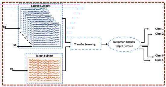
Figure 7.
Multi-source-to-single-target transfer paradigm (MTS).
5. Results
5.1. Experiment Setup for STS and MTS Transfer Paradigms
In this study, the effect of single-source-to-single-target and multi-source-to-single-target transfer learning schemes on the prediction rate is investigated, mainly to address the challenge of significant variations emanating from domain shifts between EEG recordings, in turn resulting in poor prediction rates [56]. To facilitate the investigation, domain adaption algorithms including machine learning algorithms are evaluated and contrasted with a focus on a multi-class cross-subject classification scenario. All algorithms are evaluated and contrasted under both the STS and MTS transfer learning paradigms. In this case, both the MEKT and MMFT frameworks are first extended from a two-class classification scenario to a multi-class classification case, also modified to suit both the STS and MTS experiments. When MEKT and MMFT are implemented under the STS TL scheme, a single subject is assigned as a source domain (SD), while another single subject is assigned as a target domain (TD).
Moreover, when both domain adaptation algorithms are employed, several parameters are put in place, with samples acquired from multiple multi-class subjects denoted by (z), including the corresponding class labels denoted by (y). The source domain samples are denoted by (); the corresponding class labels for the source domains are denoted by (); the predicted class labels for the TD are denoted by (); and the corresponding samples for the target domain are denoted by (). As such, MMFT and MEKT iterate through all domains, assigning a single subject as the SD, while the same subject is assigned as the TD in each iteration. In this instance, nine subjects including the corresponding class labels are utilized as input parameters when both MMFT and MEKT are executed under the STS transfer paradigm, whereby an individual subject is assigned as the SD while another single subject as the TD. The algorithms iterate through eight subjects, with each single subject assigned as the SD while the same subject is assigned as the TD in each iteration. Furthermore, under the MTS TL scheme, a single subject is assigned as a TD while the remaining eight subjects are assigned as SDs when both MEKT and MMFT are employed. Notably, similar parameters as in STS are put in place under the MTS TL scheme, including the number of iterations denoted by (N), representing the number of times both domain adaptation algorithms will loop through domains. Therefore, each of the nine subjects takes a turn as the TD. In a similar manner, when both MMFT and MEKT are executed under the MTS transfer paradigm, nine subjects including the corresponding class labels are utilized as input parameters, whereby eight subjects are assigned as the SD while a single subject as the TD. The algorithms iterate through all nine subjects, with each of the nine subjects taking a turn as the TD while the remaining eight subjects are assigned as the SDs to predict the TD in each iteration.
Notably, to reproduce the same experiments for both TL schemes when both K-NN and NB algorithms are applied through a traditional BCI framework [4,13], features from a single subject (source domain) are used for training, and features from a different individual subject (target domain) are used for prediction when both ML algorithms are employed under the STS TL scheme. Under the MTS transfer learning scheme, features from eight different subjects are used for training, while features from a different individual subject are used for prediction when both ML algorithms are applied [27,57].
5.2. Setup for SD Increment Experiment
In this experiment, a further investigation is carried out to determine whether increasing the number of SDs by an individual subject in each iteration can have a severe impact on cross-subject transfer performance. As such, the performance of domain adaptation, including ML algorithms, is contrasted and evaluated to further examine the effect of inter-subject variations in EEG characteristics on the prediction rate. Therefore, similar parameters used under the STS and MTS transfer paradigms are still used as input parameters to both the MMFT and MEKT frameworks when employed under the SD increment experiment. In this case, both domain adaptation algorithms iterate through all nine subjects, assigning the same subject as the TD in each iteration, and from the remaining eight subjects, an individual subject is first assigned as the SD while in each iteration the number of SDs is incremented by an individual subject. Notably, in the first iteration, a single subject is assigned as the SD and another subject as the TD. The number of SDs is continually incremented by an individual subject until all eight subjects are included and assigned as the TD, while the same subject initially assigned as the TD is assigned as the TD in each iteration. Moreover, to reproduce a similar experimental setup when both the K-NN and NB are employed for the SD increment experiment, a single subject is used for the prediction while the number of subjects used for training is continually incremented by an individual subject.
5.3. Experimental Results
5.3.1. Single-Source-to-Single-Target (STS) Transfer Paradigm
Performance Evaluation Under STS Transfer Paradigm Utilizing BCI Competition IV-a Dataset
In this section, the effect of the single-source-to-single-target transfer learning paradigm on cross-subject transfer performance is investigated utilizing the BCI Competition IV-a dataset consisting of nine MI subjects. Subsequently, two domain adaptation algorithms—including ML algorithms implemented through a traditional BCI pipeline—are utilized to evaluate the impact of inter-subject variations in EEG characteristics, mainly to determine the effect of domain shifts between EEG recordings contributing to significant variations, leading to a poor prediction rate. In this case, the MEKT and MMFT frameworks are introduced and contrasted with K-NN, including NB, under the STS transfer learning paradigm with a focus on a cross-subject classification scenario. Notably, when MEKT and MMFT are employed, samples from multiple diverse domains (subjects), including their corresponding class labels, are first used as input parameters, whereby an individual subject is assigned as the SD, while both algorithms individually loop through the remaining subjects, assigning a single subject as a TD in each iteration.
Figure 8 shows the prediction rates for performance evaluation based on the STS transfer learning paradigm, whereby MMFT is contrasted with MEKT—including two classical ML algorithms (K-NN and NB)—using nine MI subjects acquired from the BCI Competition IV-a dataset. The evaluation of performance in this instance was conducted to examine the impact of domain shifts between EEG recordings on the intention detection rate, mainly to mitigate the challenge of massive variations in EEG characteristics contributing to poor cross-subject transfer performance, indicated by a low intention detection rate from subject to subject.
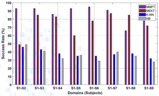
Figure 8.
Classification results for STS transfer paradigm based on BCI Competition IV-a dataset.
From the results in Figure 8, it can be noted that the domain shifts between EEG recordings contributing to variations in EEG neural dynamics have a severe impact on the performance of ML algorithms from subject to subject due to the challenge of overfitting. Hence, a significant decline in prediction rate was captured when both K-NN and NB were employed, whereby the NB classifier recorded the highest CA of 49% when the first subject (S1) was used for training and the second subject (S2) for prediction, depicted by S1–S2. Moreover, the K-NN classifier recorded the highest CA of 46% when S1 was used for training and S2 for prediction under a one-to-one transfer paradigm. Furthermore, domain adaptation algorithms were demonstrated to minimize the effect of domain shifts across EEG recordings. Hence, superior prediction rates were observed when both MEKT and MMFT assign an individual domain as an SD, while iterating through the remaining subjects and assigning a single different subject as the TD in each iteration. Notably, MMFT recorded the highest CA of 95% when S1 was assigned as the SD and S2 as the TD, while the highest CA of 85% was captured when MEKT was employed in a one-to-one transfer paradigm.
In Table 1, a comparative performance analysis is carried out using the BCI Competition IV-a dataset to evaluate the cross-subject transfer performance of domain adaptation algorithms, including ML algorithms under the STS transfer paradigm. As such, performance evaluation was conducted to mainly determine the impact of domain shifts between EEG recordings adding to significant inter-subject variations, in turn increasing the distribution shifts between the SD and TDs, leading to a decline in the prediction rate. In this case, the prediction rate of each subject was averaged to obtain the mean accuracy—when an individual subject was assigned as the SD while the remaining eight subjects were assigned as the TDs—in each iteration when MMFT, MEKT, K-NN, and NB were applied. Consequently, the MMFT framework outperformed MEKT, while both K-NN and NB classifiers were massively affected by the immense variations in EEG characteristics from subject to subject. Notably, MMFT recorded a superior mean CA of 89% when S1 was assigned as the SD, and the CA was acquired when each of the remaining eight subjects assigned as the TD in each iteration was averaged. The MEKT algorithm also yielded remarkable performance with the highest mean CA of 87% recorded across S8, while inferior mean CAs of 38% and 37% were captured across S1 and S2 when both the K-NN and NB were employed, respectively, as illustrated in Table 1.

Table 1.
Mean (%) and standard deviation (in parenthesis) of both domain adaptation and ML algorithms under STS transfer paradigm (BCI Competition IV-a).
Performance Evaluation Under STS Transfer Paradigm Utilizing the Recorded MI Dataset
The impact of the STS transfer paradigm on cross-subject transfer performance is further investigated in this section utilizing the recorded MI dataset. In a similar manner, when both domain adaptation algorithms are applied, a single subject is assigned as the SD while the algorithms also loop through the remaining eight subjects, assigning a single subject as the TD in each iteration. Moreover, to reproduce a similar one-to-one transfer paradigm when both ML algorithms are employed, an individual subject is utilized for training and another subject used for prediction. However, emulating a similar one-to-one or STS transfer paradigm when ML algorithms are employed demonstrated a severe impact on cross-subject transfer performance, denoted by the inferior intention detection rates from subject to subject.
Consequently, K-NN recorded the highest CA of 57% across S7–S1 when S7 was assigned as the SD and S1 as the TD, while NB recorded the highest CA of 49% across S7–S3 when S7 was assigned as the SD and S3 as the TD under the STS transfer paradigm. Moreover, a massive decline in the prediction rate can further be observed across individual subjects when both ML algorithms are employed, as illustrated in Figure 9. In this case, inferior performance can be attributed to significant inter-subject variations due to domain shifts between EEG recordings coupled with a low signal-to-noise ratio, in turn resulting in the challenge of overfitting.
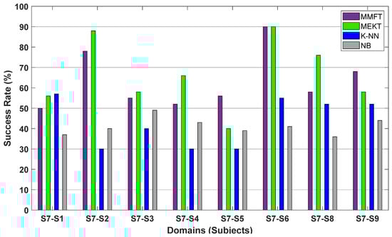
Figure 9.
Classification results for STS transfer paradigm based on the recorded MI dataset.
Notably, applying both MMFT and MEKT based on a one-to-one transfer paradigm reduced the effect of significant variations in EEG characteristics, in turn enhancing cross-subject transfer performance. Hence, a superior CA of 90% was captured for the MEKT and MMFT frameworks across S7–S6, respectively, when S7 was assigned as the SD and S6 as the TD. Furthermore, it is worth noting that looping through domains and assigning a non-identical subject as a TD in each iteration proved to massively affect the performance for cross-subject transfer due to negative transfer. Consequently, the lowest prediction rate of 50% was observed across S7–S1, while an inferior CA of 40% was captured across S7–S5 when MMFT and MEKT were applied, respectively.
Table 2 shows the results for the comparative performance analysis using the recorded MI dataset, whereby MMFT is contrasted with MEKT—including K-NN and NB classifiers—based on the STS transfer paradigm, mainly to examine the impact of domain shifts contributing to immense variation in cross-subject transfer performance. As such, the CA is acquired when an individual subject is assigned as the SD while the remaining eight subjects take turns as the TD, which is averaged to obtain the mean CA. Notably, the MMFT framework recorded a superior mean CA of 63% as compared to both K-NN and NB, with the highest mean CAs of 45%, respectively, as illustrated in Table 2. However, it is worth noting that MEKT outperformed all other algorithms and recorded a superior mean CA of 67%, acquired through averaging the CAs when each of the eight subjects is assigned as the TD and while the same subject is assigned as the SD in each iteration, and this process is repeated across each subject as an SD.
Table 2.
Mean (%) and standard deviation (in parenthesis) of both domain adaptation and ML algorithms under STS transfer paradigm (the recorded MI dataset).
Performance Evaluation Under STS Transfer Paradigm Utilizing the Recorded SSVEP Dataset
In this experiment, the recorded SSVEP dataset acquired from nine subjects is further utilized to investigate the effect of the STS transfer paradigm on cross-subject transfer performance, mainly to mitigate the challenge of massive inter-subject variations in EEG characteristics emerging from domain shifts between EEG recordings. As such, MEKT is further contrasted with the MMFT framework, including classical ML algorithms (K-NN and NB) under a one-to-one transfer paradigm. Notably, iterating through various subjects assigning a different individual subject as the TD—while the same but different subject from the TD is assigned as the SD in each iteration—further illustrated that domain adaptation algorithms can significantly enhance the prediction rate. Subsequently, a superior CA of 100% was recorded when S1 was assigned as SD and S5 as TD, denoted by S1–S5, when the MEKT and MMFT frameworks were applied in a one-to-one transfer paradigm, respectively. Moreover, massive individual differences across subjects proved to have a severe impact on cross-subject transfer performance. Consequently, a significant decrease in the prediction rate was observed across S1–S3 when a non-related domain was assigned as the TD. Hence, MEKT and MMFT recorded inferior prediction rates of 34% and 20%, respectively, when S1 was assigned as the SD and S3 as the TD, as illustrated in Figure 10.
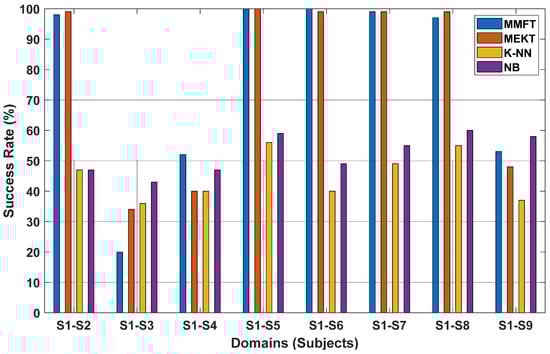
Figure 10.
Classification performance for STS transfer learning paradigm based on the recorded SSVEP dataset.
Furthermore, when contrasted with ML algorithms, domain adaptation algorithms yielded superior cross-subject transfer performance in the one-to-one transfer paradigm, while inter-subject variations illustrated that ML algorithms can be massively affected by domain shifts between EEG recordings. Hence, inferior performance was observed from subject to subject when both K-NN and NB classifiers were employed. In this case, K-NN recorded the highest CA of 56% across S1–S5 when samples from S1 were used for training and S5 for prediction, while the NB classifier recorded the highest CA of 60% across S1–S8 when S1 was used to train and S8 to predict. From the experimental results, it is worth noting that employing domain adaptation algorithms can significantly minimize the effect of domain shifts between EEG recordings that contribute to immense variations in EEG characteristics, and cross-subject transfer performance was massively affected by the transfer of non-identical domains, denoted by a decline in CAs across individual subjects.
An extensive comparative performance analysis is further conducted utilizing the recorded SSVEP dataset to evaluate the cross-subject transfer performance of domain adaptations, including ML algorithms. In this case, comparative performance evaluation is carried out between MMFT, MEKT, K-NN, and NB classifiers with a focus on the STS transfer paradigm. From the comparison, it is worth noting that immense inter-subject variations have a severe impact on the performance of ML algorithms; hence, a significant decline in CAs was observed across the individual subjects, in turn resulting in low mean CAs. Hence, the NB classifier recorded the highest mean CA of 51% while the highest mean CA of 50% was captured for K-NN, as illustrated in Table 3. However, domain adaptation algorithms minimized the effect of immense inter-subject variations, leading to a significant increase in CA. Consequently, MEKT outperforms all algorithms under the STS transfer paradigm experiment, with a superior mean CA of 82% recorded; meanwhile, MMFT recorded a mean CA of 78%. Notably, a decrease in the intention detection rate across subjects when MEKT and MMFT are employed can be attributed to the transfer of features from non-related domains possessing immense individual differences.
Table 3.
Mean (%) and standard deviation (in parenthesis) of both domain adaptation and ML algorithms under STS transfer paradigm (the recorded SSVEP).
5.3.2. Multi-Source-to-Single-Target (MTS) Transfer Learning Paradigm
Performance Evaluation Under MTS Transfer Paradigm Utilizing BCI Competition IV-a Dataset
In this section, an MTS transfer paradigm experiment is conducted to investigate the effect of domain shifts between EEG recordings on the performance of cross-subject transfer. As such, the BCI Competition IV-a dataset consisting of nine MI subjects is utilized to facilitate the investigation, mainly to examine the impact of inter-subject variations emerging from domain shifts between the EEG recordings on the prediction rate. Therefore, a comparative performance analysis was carried out between the MMFT, MEKT, and traditional ML algorithms (K-NN and NB) employed using a classical BCI pipeline. Therefore, when domain adaptation algorithms are implemented under the MTS transfer paradigm, the algorithms iterate through all nine domains, assigning eight subjects as the SDs and one different subject as the TD in each iteration; this process is repeated nine times as each subject takes a turn as the TD.
Consequently, Figure 11 displays the performance evaluation results of the MMFT when contrasted with MEKT, K-NN, and NB [34]. Results from the evaluation demonstrated that domain adaptation algorithms yield superior prediction rates between individual TD, while ML algorithms are severely affected by the challenge of overfitting, in turn resulting in inferior CAs. As such, a superior success rate of 96% was recorded when S3 was assigned as the target domain and while the remaining subjects (S1~S2 and S4~S9) were assigned as the SDs when both MMFT and MEKT were employed, respectively. However, a significant decline in CA was recorded when K-NN was employed, with the highest success rate of 48% noted when S1 was utilized for prediction while the remaining subjects (S2~S9) were utilized for training. A decrease in success rate was also noted when NB was applied, with the highest success rate of 40% observed when S8 was utilized to test while the remaining subjects (S1~S7 and S9) were utilized for training.
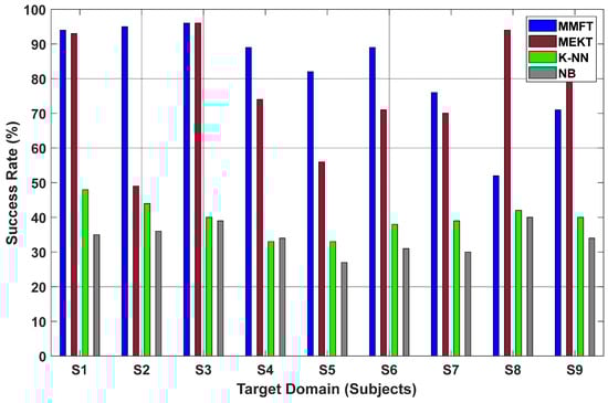
Figure 11.
Classification results for MTS transfer-paradigm-based BCI Competition IV-a dataset.
Superior prediction rates were observed when the MMFT algorithm was employed, while MEKT also yielded remarkable results. However, subjects possessing massive individual differences in EEG characteristics resulted in another significant challenge in the form of negative transfer (NT), which significantly deteriorated the prediction rate between TDs. Hence, an inferior success rate of 52% was recorded when S8 was assigned as the TD, and the remaining subjects (S1~S7 and S9) were assigned as the SDs when MMFT was employed. A massive decline in success rate was further observed when MEKT was applied, with an inferior success rate of 49% recorded when S2 was assigned as the TD while the remaining subjects (S1 and S3~S9) were assigned as the SDs. A further decline in the prediction rate as a result of the challenge of overfitting was noted when the K-NN and NB classifiers were employed. Notably, an inferior success rate of 33% was observed when S4 was utilized for prediction and the remaining subjects (S1~S3 and S5~S9) were utilized for training when K-NN was employed. Additionally, NB recorded an inferior success rate of 27% when S5 was assigned as the TD and S1~S4 and S6~S9 assigned as the SDs.
Performance Evaluation Under MTS Transfer Paradigm Utilizing the Recorded MI Dataset
In this section, nine of the recorded MI subjects are utilized to further investigate the effect of domain shifts between the EEG recordings on the performance of TL, whereby the impact of inter-subject variations on cross-subject transfer performance is examined—with a focus on the MTS transfer paradigm [58,59]. Therefore, a single subject was assigned as the TD and the remaining subjects were assigned as the SDs, while each of the nine subjects took turns as the TD when both MMFT and MEKT frameworks were applied. Figure 12 displays the results for the comparative performance analysis between MMFT, MEKT, and two traditional machine learning algorithms (K-NN and NB) for the subject-to-subject classification scenario based on the MTS transfer paradigm. In this case, the results clearly illustrated that domain adaptation frameworks can minimize the effect of inter-subject variations, in turn significantly improving the prediction rate for the subject-to-subject prediction scenario. However, reproducing similar transfer learning conditions for both K-NN and NB classifiers severely affected the performance. Hence, assigning eight subjects for training and a single subject for prediction when both K-NN and NB were applied gave rise to the challenge of overfitting.
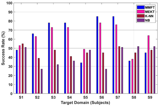
Figure 12.
Classification performance for MTS transfer learning paradigm based on the recorded MI dataset.
As such, a success rate of 52% was recorded, which is the highest across all TDs when K-NN was employed—whereby S1 was utilized for prediction and the remaining subjects (S2~S9) were utilized for training. A further decline was noted when NB was employed, with a success rate of 52% captured when S9 was utilized for prediction and the remaining subjects (S1~S8) were utilized for training the algorithm [60]. Notably, the introduction of MMFT proved to significantly enhance the prediction rate, hence, a superior success rate of 85% was captured when S6 was assigned as the TD and the remaining subjects (S1~S5 and S7~S9) were assigned as the SDs. From this comparison, it was further noted that MMFT outperformed another domain adaptation algorithm in the form of MEKT, whereby MEKT recorded a success rate of 78% when S6 was assigned as the TD and the remaining eight subjects were assigned as the SDs.
Highly beneficial domains in this instance were indicated to be effective for the MMFT, while low beneficial subjects contributed to the effect of negative transfer, denoted by significantly low prediction rates between subjects. In this case, the impact of negative transfer attributed to inter-subject variations on IDRs was demonstrated by a massive decrease in CA, with a success rate of 34% noted when S5 was assigned as the TD and the other subjects (S1~S4 and S6~S9) were assigned as the SDs when MMFT was employed. Furthermore, features from low beneficial subjects proved to severely affect the performance of both K-NN and NB. Hence, an inferior success rate of 39% was captured when S1 and S3~S9 were utilized for training and S2 was utilized for prediction when K-NN was employed. In a similar manner, an inferior success rate of 27% was captured when S1 and S3~S9 were utilized for training, while features from S2 were utilized for prediction.
The experimental results demonstrated that domain adaptation algorithms (MMFT and MEKT) can significantly minimize the effect of inter-subject variation, in turn enhancing intention detection rates for subject-to-subject classification. However, significant individual differences in neural dynamics across subjects severely affect the success rates between domains as a result of negative transfer. Hence, a poor prediction rate was noted across S1, S5, and S8~S9, as illustrated in Figure 12. Moreover, inter-subject variabilities—including BCI illiteracy—proved to massively contribute to poor intention detection rates when both domain adaptation algorithms were applied on the recorded MI dataset.
Performance Evaluation Under MTS Transfer Paradigm Utilizing the Recorded SSVEP Dataset
The MTS transfer paradigm experiment is conducted in this section using the recorded SSVEP dataset to further investigate the effect of domain shifts between EEG recordings contributing to inter-subject variation in cross-subject transfer performance. In this instance, performance evaluation is carried out mainly to mitigate the challenge of inter-subject variations in EEG characteristics that lead to poor cross-subject transfer performance [44]. As such, a comparative performance evaluation is carried out between the K-NN, NB, MEKT, and MMFT frameworks. Therefore, nine SSVEP subjects are utilized to facilitate the investigation, mainly to determine the effect of significant variations in EEG neural characteristics on performance. In this case, eight subjects were assigned as SDs and one subject as the TD, and each of the nine subjects took turns as the TD when both MMFT and MEKT were individually applied. Furthermore, eight subjects were utilized for training and one subject utilized for prediction and each of the nine subjects took turns for the prediction when K-NN and NB were applied. Results from Figure 13 show the intention detection rate of each of the four algorithms when compared.
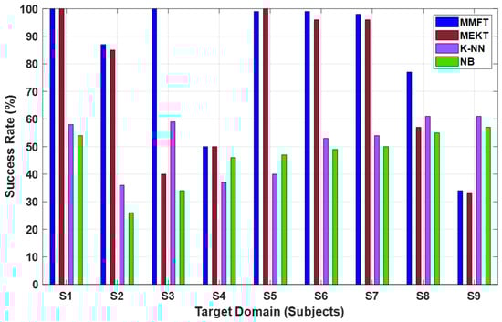
Figure 13.
Classification performance for MTS transfer learning paradigm based on the recorded SSVEP dataset.
Therefore, a superior success rate of 100% was captured when S1 was assigned as the TD and the remaining sessions (S2~S9) were assigned as the SDs when MMFT was applied. Moreover, a similar superior success rate of 100% was observed when MEKT was applied to nine SSVEP subjects where S2~S9 were assigned as SDs and S1 was assigned as the TD. However, a decrease in success rate was noted when the ML algorithms were employed, with the highest success rate of 61% recorded when K-NN was applied across S9, while NB recorded the highest success rate of 57% across S9.
The presence of low beneficial subjects when S1~S8 were assigned as SDs severely affected the transferability of features when S9 was assigned as a TD, with an inferior success rate of 34% recorded when MMFT was applied to the nine subjects. In a similar manner, subjects possessing massive individual differences in EEG characteristics further contributed to low success rates. Hence, significantly poor prediction rates were observed between S3 and S9 each time a subject took a turn as the TD when MEKT was applied, with CAs of 40% and 33% recorded, respectively. Notably, utilizing features from different subjects for training also resulted in poor prediction rates, with the lowest success rate of 36% captured across S2 when the remaining subjects were utilized for training when K-NN was applied. A decrease in prediction rate was further observed when NB was applied, with the lowest success rate of 26% recorded across S2.
It can be noted from the comparison results in Figure 13 that subject-to-subject variabilities can massively contribute to poor prediction rates between subjects. In this case, deterioration in the prediction rate can be attributed to low beneficial subjects, possessing significant individual differences in electroencephalogram neural characteristics. However, highly beneficial subjects demonstrated remarkable classification performance between subjects. Hence, superior prediction rates were observed when each of the eight subjects were assigned as the TD in the domain adaptation algorithms implemented based on the MTS transfer paradigm.
Results from Table 4 depict the cross-subject transfer performance when domain adaptation together with ML algorithms are compared under the MTS transfer paradigm. In this case, nine MI subjects acquired from the BCI Competition IV-a dataset—including the recorded MI and SSVEP datasets—were utilized for experimentation. As such, the performance in this instance was examined by employing the MMFT and MEKT, including K-NN and NB algorithms, on each of the datasets. Therefore, the performance of each dataset was evaluated based on the prediction rates of each of the four algorithms. Consequently, employing both MMFT and MEKT under the MTS transfer paradigm reduced the effect of domain shifts between EEG recordings, in turn enhancing the prediction rate. Hence, a superior mean prediction rate of 83% was recorded when the MMFT algorithm was applied, while the highest mean CA of 76% was captured when MEKT was applied on the BCI Competition IV-a dataset. However, domain shifts contributing to immense inter-subject variations massively affected the classification performance of ML algorithms, demonstrated by a decrease in the CA across individual subjects. Hence, inferior mean CAs of 40% and 34% were captured when the K-NN and NB classifiers were applied on the BCI Competition IV-a dataset, respectively. Moreover, a slight increase in CA was observed when K-NN and NB were applied on the recorded MI dataset, with mean CAs of 51% and 46%, respectively. However, MEKT and MMFT outperformed ML algorithms when applied on the recorded MI dataset, whereby MEKT recorded a mean CA of 63% and MMFT recorded a mean CA of 62%, as illustrated in Table 4. Notably, a decline in the CA when MEKT and MMFT were applied can be attributed to the transfer of features from non-related subjects possessing immense individual differences. In a similar manner, the K-NN and NB classifiers were demonstrated to be immensely affected by the effect of overfitting demonstrated by poor prediction rates, hence, inferior CAs were observed when they were employed on the recorded SSVEP dataset. In this instance, mean CAs of 46% and 42% were captured when K-NN and NB were applied, while an increase in mean CA was noted when MEKT was employed—with a mean CA of 73% captured under the MTS transfer paradigm using the recorded SSVEP dataset. Additionally, MMFT recorded a superior mean CA when contrasted with MEKT and ML algorithms under the same transfer paradigm, with a superior mean CA of 83% captured when applied on the recorded SSVEP dataset.
Table 4.
Mean (%) and standard deviation (in parenthesis) of both domain adaptation and ML algorithms under MTS transfer paradigm.
5.3.3. Impacts of Hyper Parameters
A single hyper parameter is considered in this research—which is the number of source domains for training—to evaluate whether incrementing the number of source domains for training can massively affect the classification performance when domain adaptation, including ML algorithms, is applied on three EEG datasets.
Performance Evaluation for Different Numbers of Source Domains
- (1)
- Source-domain increment experiment utilizing BCI Competition IV-a dataset
In this section, MMFT and MEKT frameworks are further modified according to the SD increment experiment, mainly to investigate whether increasing an individual subject in each iteration can pose a massive impact on the prediction rate when both domain adaptation algorithms are employed. As such, when domain adaptation algorithms are implemented, nine subjects are used as input parameters, while both algorithms iterate through all subjects assigning SDs and TDs. In the first iteration, a single subject is assigned as the SD and another subject as the TD. Moreover, in each iteration, the number of domains is incremented by an individual subject who is assigned as one of the SDs, while the same subject assigned as the TD in the first iteration is assigned as the TD in each iteration. This procedure was repeated nine times as each subject took turns as the TD. To emulate a similar SD increment experiment using ML algorithms, the number of subjects used for training is incremented by an individual subject while a single subject is used for prediction. Initially, when both K-NN and NB are employed, a single subject is used for training and another subject for prediction; then, the number of subjects used for training is continually incremented by a different individual subject until all eight subjects are used for training—simultaneously, the same subject initially used for the prediction is used for the prediction each time that the number of subjects is incremented.
The experimental results depicted in Figure 14 illustrate that incrementing the number of SDs in each iteration can massively enhance the prediction rate when domain adaptation algorithms are employed. Hence, MEKT and MMFT recorded inferior CAs of 84% and 90%, respectively, in the first iteration when a single subject was assigned as the SD and another subject assigned as the TD. However, incrementing the number of SDs by an individual subject resulted in an increase in the CA in each iteration, with a superior CA of 97% recorded when MMFT and MEKT were applied, as illustrated in Figure 14.
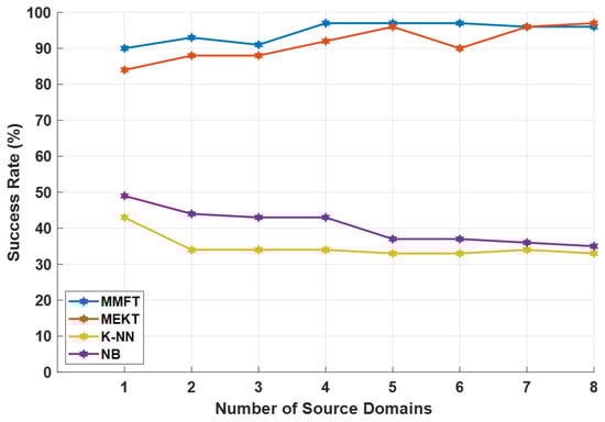
Figure 14.
Performance evaluation based on source-domain increments using BCI Competition IV-a dataset.
Additionally, incrementing the number of subjects used for training immensely deteriorates the prediction rate when the ML algorithms are applied. Hence, inferior CAs of 33% and 35% were observed when eight subjects were used to train and a single subject used to predict when K-NN and NB were applied, respectively. Notably, an increase in CA can be noted when a single subject is used for training and a single subject used for prediction; hence, CAs of 43% and 49% were initially captured when K-NN and NB were applied.
- (2)
- Source-domain increment experiment utilizing the recorded MI dataset
In this experiment, domain adaptation—including ML algorithms—is further employed on the recorded MI dataset to examine whether increasing the number of domains in each iteration can significantly affect the cross-subject transfer performance. In this instance, the MMFT framework is contrasted with MEKT, including the K-NN and NB classifiers, under similar experimental conditions for the SD increment experiment, mainly to evaluate the impact of immense inter-subject variations emerging from domain shifts between the EEG recordings on cross-subject transfer performance. Moreover, it is worth noting that all nine experiment subjects for the recorded MI dataset had no prior BCI training, hence, low prediction rates were noted due to BCI literacy. From the results in Figure 15, it can be noted that significant individual differences across domains due to immense variations in EEG characteristics can massively deteriorate the prediction rate. Such immense variations in EEG neural dynamics can also be attributed to BCI literacy due to a lack of prior BCI training for the MI subjects.
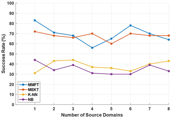
Figure 15.
Performance evaluation based on source-domain increments using the recorded MI dataset.
Hence, a decline in the prediction rate was observed from the first until the fourth iteration (1~4), when MMFT was employed, while incrementing the number of individual subjects in each iteration. However, incrementing the number of domains proved beneficial across the fourth until the sixth iteration (4~6), hence, an increase in the prediction rate was noted. A CA of 56% was captured in the fourth iteration and a CA of 78% was observed in the sixth iteration when MMFT was employed. Notably, domains possessing a massive similarity in EEG characteristics are also demonstrated to enhance CA. Hence, MMFT recorded a superior CA of 83% in the first iteration when a single subject was assigned as an SD and another subject as a TD. MEKT, on the other hand, maintained fluctuating CAs, with slight declines and increases observed across each iteration when the number of SDs was incremented. However, MEKT recorded the highest CA of 72% in the first iteration when a single subject was assigned as an SD and another subject as a TD, as depicted in Figure 15. Furthermore, when K-NN and NB are employed under the same SD-increment experimental procedure, a decline in CA is observed across 3~6 as the number of subjects is incremented, while NB recorded the highest CA of 44% compared to K-NN when a single subject was used for training and another single subject for prediction.
- (3)
- Source-domain increment experiment utilizing the recorded SSVEP dataset
The effect of the immense variation in EEG characteristics from subject to subject is further evaluated to determine whether incrementing SDs by an individual subject can enhance the performance for cross-subject transfer. Therefore, to facilitate the investigation the recorded SSVEP dataset is used to further examine the impact of domain shifts between EEG recordings contributing to immense inter-subject variations. As such, MMFT is compared with MEKT, including two ML classifiers (K-NN and NB), under the same experimental conditions for the SD increment experiment. From the results in Figure 16, it can be noted that incrementing the number of individual subjects in each iteration can enhance the performance of cross-subject transfer, while the presence of non-related domains possessing immense individual differences deteriorated the CA when domain adaptation algorithms were employed.
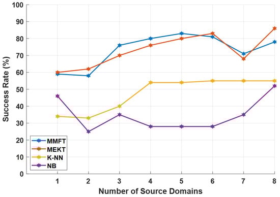
Figure 16.
Performance evaluation based on source-domain increments using the recorded SSVEP dataset.
Notably, a massive increase in CA was observed from the first until the sixth iteration (1~6) when the number of SDs was incremented by an individual subject each time. In this case, a CA of 60% was observed across the first iteration when a single subject was assigned as the SD, while a CA of 83% was captured across the sixth iteration when MEKT was employed and assigned six subjects as the SDs. Moreover, when MMFT was employed, an increase in CA was observed from the second until the fifth iteration (2~5), with a CA of 58% captured when two subjects were assigned as SDs, 25% in CA noted when five subjects were assigned as SDs, and with an accuracy of 83% recorded. Furthermore, the K-NN classifier demonstrated a slight increase and maintained slightly similar CAs across 4~8 when applied on the recorded SSVEP dataset. An increase in CA from 34% to 54% was observed across 1~4 when training samples were incremented by a single subject in each iteration when K-NN was applied. Inferior performance was observed when NB was employed and the number of training samples was incremented by an individual subject in each iteration. An increase in CA in this instance can be attributed to individual subjects possessing massive similarities in their EEG neural characteristics.
The experimental results demonstrated that employing domain adaptation algorithms can minimize the effect of inter-subject variations, in turn enhancing cross-subject transfer performance when samples from multiple subjects are used as SDs. Moreover, the results also illustrated that non-related subjects possessing immense individual differences in EEG neural characteristics can deteriorate the prediction rate from subject to subject. These results further support that domain shifts between EEG recordings do contribute to significant inter-subject variations and can massively affect cross-subject transfer performance.
5.3.4. Computational Complexity
The computational complexity was measured in this section by evaluating the processing time of each of the four algorithms under three-class prediction scenarios, as illustrated in Table 5. In this case, when the computational complexity was examined, nine EEG subjects acquired from our own recorded SSVEP dataset were used to facilitate the investigation. From Table 5, it can be noted that low computational time or processing time was captured when domain adaptation algorithms were applied. Hence, the lowest processing time of 9.1 s seconds was observed when MMFT was employed for inter-subject prediction. Moreover, the MEKT recorded a low computational time of 9.4 s for inter-subject prediction under the MTS transfer paradigm, while both NB and K-NN recorded lowest the computational times of 214.6 s and 224.2 s, respectively. However, iterating through domains, assigning an individual subject as the SD while another subject is assigned as the TD in each iteration, increased the processing time under STS when all four algorithms were employed. Hence, processing times of 1586.4 s and 1994.4 s were captured for both NB and K-NN, while employing MEKT and MMFT resulted in processing times of 16.7 s and 14.8 s, respectively.
Table 5.
Computational complexity of the four algorithms under STS and MTS.
6. Discussion
The transferability of features across domains is highly significant for enhancing the cross-subject transfer performance when domain adaptation algorithms are employed based on cross-subject classification scenarios. Hence, features extracted from samples in the source domain are utilized to improve the learning performance in the TD. However, domain shifts between EEG recordings can massively contribute to the challenge of inter-subject variations in EEG characteristics, in turn drastically deteriorating the prediction rates from subject to subject. Moreover, immense domain shifts between EEG recordings further contribute to the massive individual differences between subjects, in turn increasing the distribution shifts between the source and target domains, resulting in poor cross-subject transfer performance [13].
In this study, the effect of domain shifts between the EEG recordings contributing to significant individual differences in EEG neural characteristics on cross-subject transfer performance is investigated. As such, the BCI Competition IV-a dataset—including the recorded MI and SSVEP datasets—was utilized to facilitate the investigation, mainly to determine the impact of the domain shift between the EEG recordings on the prediction rate, and, at the same time, mitigate the challenge of immense inter-subject variations in EEG characteristics [61]. Subsequently, to examine the effect of domain shifts between EEG recordings on cross-subject transfer performance, a comparative performance analysis was carried out between domain adaptation algorithms and classical ML algorithms. In this case, the MMFT framework was introduced and contrasted with MEKT, including K-NN and NB, under the STS and MTS transfer paradigms. Notably, under the STS transfer paradigm experiment, both MMFT and MEKT received nine subjects—including the corresponding class labels—as input parameters, then it iterated through all nine domains assigning a different individual subject as the SD in each iteration while the same subject was assigned as the TD in each iteration [33,34]. This process was repeated until the number of iterations reached nine subjects, and when the number of iterations reached nine subjects, the number of iterations started again from one with a new subject as a TD. Moreover, under the MTS transfer paradigm experiment, the same input parameters as in the STS experiment were utilized. However, both the MMFT and MEKT frameworks first assigned a single subject as the TD and the remaining subjects assigned as SDs, in this instance, each of the nine subjects took turns as the TD while the same process was repeated in each iteration. The same STS and MTS transfer paradigm experiments were reproduced when the ML algorithms were employed, mainly to establish a fair contrast between MMFT, MEKT, K-NN, and NB classifiers.
Consequently, subjects possessing significant individual differences in EEG characteristics due to immense domain shifts between the EEG recordings massively affected the performance of ML algorithms under the STS transfer paradigm experiment. Hence, a drastic decline in CAs was observed from subject to subject, which translated to highest mean CAs of 38% and 37% when both the K-NN and NB classifiers were applied on the BCI Competition IV-a dataset, as depicted in Table 1. Similarly, applying K-NN and NB on the recorded MI dataset also yielded inferior performance, while a slight increase in the CAs was observed when both ML algorithms were applied on the SSVEP dataset [27]. In this case, K-NN recorded mean CAs of 45% and 50% while NB achieved mean CAs of 45% and 52% when applied on both the recorded MI and SSVEP datasets, respectively, as depicted in Table 2 and Table 3. Notably, implementing domain adaptation algorithms based on the STS transfer paradigm proved to reduce the effect of significant individual differences in EEG characteristics, with a superior mean CA of 89% noted when MMFT was applied and a mean CA of 87% when MEKT was applied on the BCI Competition IV-a dataset. A decline was further noted when domain adaptation algorithms were applied on the recorded MI dataset, in this instance, the decrease in CA can be attributed to a lack of prior BCI training from all nine experimental subjects. However, MMFT and MEKT outperformed both ML algorithms with mean CAs of 63% and 67% recorded. Moreover, the results from Table 3 further illustrated that domain adaptation algorithms can massively enhance the prediction rate across individual subjects. As such, a superior mean CA of 82% was observed when MEKT was applied and MMFT recorded a mean CA of 78% when applied on the SSVEP dataset.
Additionally, the impact of inter-subject variations in EEG neural dynamics was further investigated under the MTS transfer paradigm experiment, mainly to determine the effect of domain shifts between EEG recordings on cross-subject transfer performance. As such, utilizing samples from various subjects to train and samples from a single different subject to predict when ML algorithms were applied proved to drastically deteriorate the CAs. The decline in prediction rates in this instance can be attributed to two critical challenges, including inter-subject variations in EEG characteristics emerging from domain shifts between the EEG recordings and overfitting due to individual differences in EEG characteristics from subject to subject. Hence, a significant decrease was observed across all three datasets, with inferior performance noted from subject to subject when ML algorithms were employed under the MTS transfer paradigm experiment. In this case, the highest mean CAs were observed when both K-NN and NB classifiers were applied on the recorded MI dataset, with mean CAs of 51% and 46% captured, as depicted in Table 4 [27,62]. Notably, introducing domain adaptation algorithms to mitigate the challenge of inter-subject variations in EEG characteristics reduced the effect of the domain shifts between the EEG recordings. Hence, utilizing samples from multiple subjects possessing individual differences as SDs to predict the TD illustrated that domain adaptation algorithms can enhance the transferability of features across domains. A superior CA of 100% was observed when S1 was assigned as the TD and the remaining subjects as SDs when both MMFT and MEKT were applied, as depicted in Figure 13. In this instance, the classification performance across individual TDs translated to a mean CA of 83% when MMFT was employed, while MEKT recorded a mean CA of 73% when applied on the SSVEP dataset. A comparative performance analysis using the BCI Competition IV-a dataset further illustrated that compared to traditional ML algorithms, domain adaptation algorithms can enhance the transferability of features across domains by minimizing the effect of inter-subject variations. A superior CA of 96% was noted when S3 was assigned as a TD and the remaining subjects as SDs for both domain adaptation algorithms, while the CAs across each TD translated to mean CAs of 83% and 76% when MMFT and MEKT were applied on the BCI Competition IV-a dataset, respectively. To note, factors such as concentration and mental fatigue due to a lack of prior BCI training for experiment subjects proved to contribute to a decrease in CA when all algorithms were employed on the MI dataset. However, domain adaptation algorithms recorded superior CAs compared to traditional ML algorithms, whereby MMFT recorded the highest CA of 85% across all individual TDs, while MEKT achieved a CA of 78% when S6 was assigned as the TD and the remaining subjects as SDs, as depicted in Figure 12. The classification performance across individual TDs translated to mean CAs of 62% and 63% captured when MMFT and MEKT were applied on the MI dataset [33,34].
Furthermore, evaluation of the cross-subject transfer performance under the domain-increment experiment illustrated that assigning multiple subjects as SDs can massively enhance the prediction rate compared to assigning fewer subjects as SDs. Hence, incrementing an individual subject in each iteration increased the prediction rate when MMFT and MEKT were applied, while ML algorithms showed a slight increase in CA when a single subject was used to train and another subject to predict. Nonetheless, incrementing the number of subjects used for the training proved to decrease the prediction rate when K-NN and NB were applied, as depicted in Figure 14, Figure 15 and Figure 16. Moreover, it is worth noting that MMFT applied the distribution mean alignment to enhance the transferability of domains, while MEKT utilized the covariance matrix centroid alignment to reduce the marginal probability distribution shift of different domains, enabling transferability between domains. Hence, superior CAs were recorded when both domain adaptation algorithms were employed. However, ML algorithms relied on the best selected feature subsets from subjects possessing immense individual differences in EEG characteristics, hence, inferior CAs were captured due to the challenge of overfitting. Notably, utilizing two components in the form of marginal probability distribution shift minimization and EEG trial whitening when MEKT applies the covariance matrix centroid alignment significantly improved the CAs. Hence, MEKT recorded superior prediction rates across most TDs and outperformed MMFT, including ML algorithms for one-to-one transfer. However, applying the KL divergence to minimize discrepancies between the SD and TD when MMFT applied the distribution mean alignment proved to massively enhance CAs. Hence, MMFT recorded superior performance and outperformed the other algorithms in most instances under the MTS transfer paradigm.
These results further validated that domain adaptation algorithms can enhance the transferability of features acquired from subjects with massive individual differences by reducing the effect of inter-subject variations in EEG characteristics emerging from domain shifts between EEG recordings, in turn significantly improving classification performance across individual TDs. Hence, superior cross-subject transfer performance was recorded when both the MMFT and MEKT frameworks were employed under the STS and MTS transfer paradigms. However, inter-subject variations in EEG neural dynamics had a severe impact on the performance of the ML algorithms due to the challenge of overfitting.
The development of a robust domain adaptation algorithm that integrates domain selection techniques and transfer mapping—to first evaluate the relationship between domains and then select only highly beneficial domains to minimize the negative transfer during transfer learning—represents a compelling direction to improve the adaptability and CA of EEG-based BCI systems.
7. Conclusions
In this paper, the impact of single-source-to-single-target and multi-source-to-single-target transfer paradigms on the prediction rate—with a focus on cross-subject classification—was investigated, mainly to address the challenge of significant variations in EEG characteristics emanating from domain shifts between EEG recordings, in turn leading to poor performance. To facilitate the investigation, two domain adaptions (MMFT and MEKT) including two ML algorithms (K-NN and NB), implemented through a traditional BCI pipeline, were introduced and compared utilizing three EEG datasets. In this case, all four algorithms were evaluated and contrasted under both the STS and MTS transfer learning paradigms. Consequently, applying covariance matrix centroid alignment when MEKT was employed significantly minimized the effect of domain shifts between EEG recordings. Hence, superior performance was recorded when MEKT was applied on both the recorded MI and SSVEP datasets to mitigate the challenge of inter-subject variations, while MMFT recorded superior performance when the BCI Competition IV-a dataset was utilized under the STS transfer paradigm.
Notably, employing distribution mean alignment when the MMFT framework was employed massively reduced the effect of immense inter-subject variations, resulting in superior performance under the MTS transfer paradigm. However, domain shifts between the EEG recordings massively deteriorated the CA of traditional ML algorithms for cross-subject classification due to the challenge of overfitting; hence, inferior CAs were recorded when both K-NN and NB were employed under STS and MTS transfer paradigms.
The experimental results confirmed that MMFT outperformed the state-of-the-art methods under the MTS transfer paradigm, illustrating its viability as a solution for the immense inter-subject variations. The MEKT also yielded remarkable performance under the STS transfer paradigm, further validating that domain adaptation algorithms are a viable solution for cross-subject classification.
Author Contributions
Conceptualization, R.C.M.; Methodology, R.C.M.; Software, R.C.M. and S.D.; Validation, R.C.M. and S.D.; Formal analysis, R.C.M.; Investigation, R.C.M.; Resources, P.A.O.; Writing—original draft, R.C.M.; Writing—review & editing, C.T. and S.D.; Supervision, C.T., P.A.O. and S.D.; Project administration, C.T., P.A.O. and S.D.; Funding acquisition, C.T. and P.A.O. All authors have read and agreed to the published version of the manuscript.
Funding
This research is supported by National Research Foundation of South Africa (Grant Numbers 145975 and 138429).
Data Availability Statement
The datasets used/or analyzed during the current study are publicly available online and from the corresponding author upon reasonable request.
Conflicts of Interest
The authors declare no conflict of interest.
References
- Maswanganyi, C.; Tu, C.; Owolawi, P.; Du, S. Overview of artifacts detection and elimination methods for BCI using EEG. In Proceedings of the 2018 IEEE 3rd International Conference on Image, Vision and Computing (ICIVC), Chongqing, China, 27–29 June 2018; pp. 832–836. [Google Scholar]
- Khushaba, R.N.; Al-Ani, A.; Al-Jumaily, A. Feature subset selection using differential evolution and a statistical repair mechanism. Expert Syst. Appl. 2011, 38, 11515–11526. [Google Scholar] [CrossRef]
- Maswanganyi, C.; Tu, C.; Owolawi, P.; Du, S. Discrimination of motor imagery task using wavelet based EEG signal features. In Proceedings of the 2018 International Conference on Intelligent and Innovative Computing Applications (ICONIC), Mon Tresor, Mauritius, 6–7 December 2018; pp. 1–4. [Google Scholar]
- Myrden, A.; Chau, T. A passive EEG-BCI for single-trial detection of changes in mental state. IEEE Trans. Neural Syst. Rehabil. Eng. 2017, 25, 345–356. [Google Scholar] [CrossRef]
- Saha, S.; Ahmed, K.I.; Mostafa, R.; Khandoker, A.H.; Hadjileontiadis, L. Enhanced inter-subject brain computer interface with associative sensorimotor oscillations. Healthc. Technol. Lett. 2017, 4, 39–43. [Google Scholar] [CrossRef]
- Bi, J.; Chu, M. TDLNet: Transfer data learning network for cross-subject classification based on multiclass upper limb motor imagery EEG. IEEE Trans. Neural Syst. Rehabil. Eng. 2023, 31, 3958–3967. [Google Scholar] [CrossRef]
- She, Q.; Zhang, C.; Fang, F.; Ma, Y.; Zhang, Y. Multisource Associate Domain Adaptation for Cross-Subject and Cross-Session EEG Emotion Recognition. IEEE Trans. Instrum. Meas. 2023, 72, 2515512. [Google Scholar] [CrossRef]
- Gaur, P.; Chowdhury, A.; McCreadie, K.; Pachori, R.B.; Wang, H. Logistic Regression with Tangent Space-Based Cross-Subject Learning for Enhancing Motor Imagery Classification. IEEE Trans. Cogn. Dev. Syst. 2021, 14, 1188–1197. [Google Scholar] [CrossRef]
- Luo, J.; Cui, W.; Xu, S.; Wang, L.; Chen, H.; Li, Y. A Cross-Scale Transformer and Triple-View Attention Based Domain-Rectified Transfer Learning for EEG Classification in RSVP Tasks. IEEE Trans. Neural Syst. Rehabil. Eng. 2024, 32, 672–683. [Google Scholar] [CrossRef]
- Zhang, H.; Zuo, T.; Chen, Z.; Wang, X.; Sun, P.Z. Evolutionary Ensemble Learning for EEG-based Cross-Subject Emotion Recognition. IEEE J. Biomed. Health Inform. 2024, 28, 3872–3881. [Google Scholar] [CrossRef]
- Lin, H. Artificial Intelligence with Great Potential in Medical Informatics: A Brief Review. Medinformatics 2024, 1, 2–9. [Google Scholar] [CrossRef]
- Lee, D.-Y.; Jeong, J.-H.; Lee, B.-H.; Lee, S.-W. Motor imagery classification using inter-task transfer learning via a channel-wise variational autoencoder-based convolutional neural network. IEEE Trans. Neural Syst. Rehabil. Eng. 2022, 30, 226–237. [Google Scholar] [CrossRef]
- Wang, H.; Sun, Y.; Wang, F.; Cao, L.; Zhou, W.; Wang, Z.; Chen, S. Cross-subject assistance: Inter-and intra-subject maximal correlation for enhancing the performance of SSVEP-based BCIs. IEEE Trans. Neural Syst. Rehabil. Eng. 2021, 29, 517–526. [Google Scholar] [CrossRef] [PubMed]
- Huang, J.; Zhang, Z.-Q.; Xiong, B.; Wang, Q.; Wan, B.; Li, F.; Yang, P. Cross-subject transfer method based on domain generalization for facilitating calibration of SSVEP-based BCIs. IEEE Trans. Neural Syst. Rehabil. Eng. 2023, 31, 3307–3319. [Google Scholar] [CrossRef] [PubMed]
- Chattopadhyay, S. Decoding Medical Diagnosis with Machine Learning Classifiers. Medinformatics 2024. Available online: https://ojs.bonviewpress.com/index.php/MEDIN/article/view/2583/905 (accessed on 24 February 2025). [CrossRef]
- Jeng, P.-Y.; Wei, C.-S.; Jung, T.-P.; Wang, L.-C. Low-dimensional subject representation-based transfer learning in EEG decoding. IEEE J. Biomed. Health Inform. 2020, 25, 1915–1925. [Google Scholar] [CrossRef]
- Wei, M.; Yang, R.; Huang, M.; Ni, J.; Wang, Z.; Liu, X. Sub-band cascaded csp-based deep transfer learning for cross-subject lower limb motor imagery classification. IEEE Trans. Cogn. Dev. Syst. 2023, 16, 1172–1185. [Google Scholar] [CrossRef]
- Farokhah, L.; Sarno, R.; Fatichah, C. Cross-subject channel selection using modified relief and simplified CNN-based deep learning for EEG-based emotion recognition. IEEE Access 2023, 11, 110136–110150. [Google Scholar] [CrossRef]
- Li, Z.; Zhu, E.; Jin, M.; Fan, C.; He, H.; Cai, T.; Li, J. Dynamic domain adaptation for class-aware cross-subject and cross-session EEG emotion recognition. IEEE J. Biomed. Health Inform. 2022, 26, 5964–5973. [Google Scholar] [CrossRef]
- Saha, S.; Ahmed, K.I.U.; Mostafa, R.; Hadjileontiadis, L.; Khandoker, A. Evidence of variabilities in EEG dynamics during motor imagery-based multiclass brain–computer interface. IEEE Trans. Neural Syst. Rehabil. Eng. 2017, 26, 371–382. [Google Scholar] [CrossRef]
- Wei, X.; Ortega, P.; Faisal, A.A. Inter-subject deep transfer learning for motor imagery EEG decoding. In Proceedings of the 2021 10th International IEEE/EMBS Conference on Neural Engineering (NER), Sorrento, Italy, 4–6 May 2021; pp. 21–24. [Google Scholar]
- Li, A.; Wang, Z.; Zhao, X.; Xu, T.; Zhou, T.; Hu, H. MDTL: A Novel and Model-Agnostic Transfer Learning Strategy for Cross-Subject Motor Imagery BCI. IEEE Trans. Neural Syst. Rehabil. Eng. 2023, 31, 1743–1753. [Google Scholar] [CrossRef]
- Duan, T.; Chauhan, M.; Shaikh, M.A.; Chu, J.; Srihari, S. Ultra efficient transfer learning with meta update for cross subject EEG classification. arXiv 2020, arXiv:2003.06113. [Google Scholar]
- Zhi, H.; Yu, Z.; Yu, T.; Gu, Z.; Yang, J. A multi-domain convolutional neural network for EEG-based motor imagery decoding. IEEE Trans. Neural Syst. Rehabil. Eng. 2023, 31, 3988–3998. [Google Scholar] [CrossRef] [PubMed]
- Nicolas-Alonso, L.F.; Corralejo, R.; Gomez-Pilar, J.; Álvarez, D.; Hornero, R. Adaptive stacked generalization for multiclass motor imagery-based brain computer interfaces. IEEE Trans. Neural Syst. Rehabil. Eng. 2015, 23, 702–712. [Google Scholar] [CrossRef] [PubMed]
- Rathee, D.; Raza, H.; Prasad, G.; Cecotti, H. Current source density estimation enhances the performance of motor-imagery-related brain–computer interface. IEEE Trans. Neural Syst. Rehabil. Eng. 2017, 25, 2461–2471. [Google Scholar] [CrossRef]
- Osuagwu, B.A.; Zych, M.; Vuckovic, A. Is implicit motor imagery a reliable strategy for a brain–computer interface? IEEE Trans. Neural Syst. Rehabil. Eng. 2017, 25, 2239–2248. [Google Scholar] [CrossRef]
- Yu, T.; Xiao, J.; Wang, F.; Zhang, R.; Gu, Z.; Cichocki, A.; Li, Y. Enhanced motor imagery training using a hybrid BCI with feedback. IEEE Trans. Biomed. Eng. 2015, 62, 1706–1717. [Google Scholar] [CrossRef]
- Maswanganyi, R.C.; Tu, C.; Owolawi, P.A.; Du, S. Statistical Evaluation of Factors Influencing Inter-Session and Inter-Subject Variability in EEG-Based Brain Computer Interface. IEEE Access 2022, 10, 96821–96839. [Google Scholar] [CrossRef]
- Wang, Y.; Chen, X.; Gao, X.; Gao, S. A benchmark dataset for SSVEP-based brain–computer interfaces. IEEE Trans. Neural Syst. Rehabil. Eng. 2016, 25, 1746–1752. [Google Scholar] [CrossRef]
- Zhang, Y.; Xie, S.Q.; Shi, C.; Li, J.; Zhang, Z.-Q. Cross-subject transfer learning for boosting recognition performance in SSVEP-based BCIs. IEEE Trans. Neural Syst. Rehabil. Eng. 2023, 31, 1574–1583. [Google Scholar] [CrossRef]
- Gao, Z.; Yuan, T.; Zhou, X.; Ma, C.; Ma, K.; Hui, P. A deep learning method for improving the classification accuracy of SSMVEP-based BCI. IEEE Trans. Circuits Syst. II Express Briefs 2020, 67, 3447–3451. [Google Scholar] [CrossRef]
- Zhang, W.; Wu, D. Manifold embedded knowledge transfer for brain-computer interfaces. IEEE Trans. Neural Syst. Rehabil. Eng. 2020, 28, 1117–1127. [Google Scholar] [CrossRef]
- She, Q.; Cai, Y.; Du, S.; Chen, Y. Multi-source manifold feature transfer learning with domain selection for brain-computer interfaces. Neurocomputing 2022, 514, 313–327. [Google Scholar] [CrossRef]
- Masoomi, R.; Khadem, A. Enhancing LDA-based discrimination of left and right hand motor imagery: Outperforming the winner of BCI Competition II. In Proceedings of the 2015 2nd International Conference on Knowledge-Based Engineering and Innovation (KBEI), Tehran, Iran, 5–6 November 2015; pp. 392–398. [Google Scholar]
- Hamm, J.; Lee, D.D. Grassmann discriminant analysis: A unifying view on subspace-based learning. In Proceedings of the 25th International Conference on Machine Learning, Helsinki, Finland, 5–9 July 2008; pp. 376–383. [Google Scholar]
- Cui, J.; Jin, X.; Hu, H.; Zhu, L.; Ozawa, K.; Pan, G.; Kong, W. Dynamic distribution alignment with dual-subspace mapping for cross-subject driver mental state detection. IEEE Trans. Cogn. Dev. Syst. 2021, 14, 1705–1716. [Google Scholar] [CrossRef]
- Kuang, J.; Xu, G.; Tao, T.; Wu, Q. Class-imbalance adversarial transfer learning network for cross-domain fault diagnosis with imbalanced data. IEEE Trans. Instrum. Meas. 2021, 71, 3501111. [Google Scholar] [CrossRef]
- Li, J.; Qiu, S.; Shen, Y.-Y.; Liu, C.-L.; He, H. Multisource transfer learning for cross-subject EEG emotion recognition. IEEE Trans. Cybern. 2019, 50, 3281–3293. [Google Scholar] [CrossRef]
- Lestari, F.P.A.; Pane, E.S.; Suprapto, Y.K.; Purnomo, M.H. Wavelet based-analysis of alpha rhythm on eeg signal. In Proceedings of the 2018 International Conference on Information and Communications Technology (ICOIACT), Yogyakarta, Indonesia, 6–7 March 2018; pp. 719–723. [Google Scholar]
- Alizadeh, N.; Afrakhteh, S.; Mosavi, M.R. Multi-task EEG signal classification using correlation-based IMF selection and multi-class CSP. IEEE Access 2023, 11, 52712–52725. [Google Scholar] [CrossRef]
- González-Castañeda, E.F.; Torres-García, A.A.; Reyes-García, C.A.; Villaseñor-Pineda, L. Sonification and textification: Proposing methods for classifying unspoken words from EEG signals. Biomed. Signal Process. Control 2017, 37, 82–91. [Google Scholar] [CrossRef]
- Bono, V.; Das, S.; Jamal, W.; Maharatna, K. Hybrid wavelet and EMD/ICA approach for artifact suppression in pervasive EEG. J. Neurosci. Methods 2016, 267, 89–107. [Google Scholar] [CrossRef]
- Chen, Y.; Yang, R.; Huang, M.; Wang, Z.; Liu, X. Single-source to single-target cross-subject motor imagery classification based on multisubdomain adaptation network. IEEE Trans. Neural Syst. Rehabil. Eng. 2022, 30, 1992–2002. [Google Scholar] [CrossRef]
- Zhuang, J.; Yin, G. Motion control of a four-wheel-independent-drive electric vehicle by motor imagery EEG based BCI system. In Proceedings of the 2017 36th Chinese Control Conference (CCC), Dalian, China, 26–28 July 2017; pp. 5449–5454. [Google Scholar]
- Pattnaik, P.K.; Sarraf, J. Brain Computer Interface issues on hand movement. J. King Saud Univ.—Comput. Inf. Sci. 2018, 30, 18–24. [Google Scholar] [CrossRef]
- Zhang, H.; Yang, H.; Guan, C. Bayesian learning for spatial filtering in an EEG-based brain–computer interface. IEEE Trans. Neural Netw. Learn. Syst. 2013, 24, 1049–1060. [Google Scholar] [CrossRef]
- Wang, D.; Liu, Z.; Tao, Y.; Chen, W.; Chen, B.; Wang, Q.; Yan, X.; Wang, G. Improvement in EEG source imaging accuracy by means of wavelet packet transform and subspace component selection. IEEE Trans. Neural Syst. Rehabil. Eng. 2021, 29, 650–661. [Google Scholar] [CrossRef] [PubMed]
- Bong, S.Z.; Wan, K.; Murugappan, M.; Ibrahim, N.M.; Rajamanickam, Y.; Mohamad, K. Implementation of wavelet packet transform and non linear analysis for emotion classification in stroke patient using brain signals. Biomed. Signal Process. Control 2017, 36, 102–112. [Google Scholar] [CrossRef]
- Alickovic, E.; Kevric, J.; Subasi, A. Performance evaluation of empirical mode decomposition, discrete wavelet transform, and wavelet packed decomposition for automated epileptic seizure detection and prediction. Biomed. Signal Process. Control 2018, 39, 94–102. [Google Scholar] [CrossRef]
- Abduallatif, N.A.; Elsherbini, S.G.; Boshra, B.S.; Yassine, I.A. Brain-Computer Interface controlled functional electrical stimulation system for paralyzed arm. In Proceedings of the 2016 8th Cairo International Biomedical Engineering Conference (CIBEC), Cairo, Egypt, 15–17 December 2016; pp. 48–51. [Google Scholar]
- Bak, S.; Jeong, J. User biometric identification methodology via EEG-based motor imagery signals. IEEE Access 2023, 11, 41303–41314. [Google Scholar] [CrossRef]
- Sai, C.Y.; Mokhtar, N.; Arof, H.; Cumming, P.; Iwahashi, M. Automated classification and removal of EEG artifacts with SVM and wavelet-ICA. IEEE J. Biomed. Health Inform. 2018, 22, 664–670. [Google Scholar] [CrossRef]
- Lahiri, R.; Rakshit, P.; Konar, A. Evolutionary perspective for optimal selection of EEG electrodes and features. Biomed. Signal Process. Control 2017, 36, 113–137. [Google Scholar] [CrossRef]
- Akuthota, S.; Rajkumar, K.; Ravichander, J. EEG based Motor Imagery BCI using Four Class Iterative Filtering & Four Class Filter Bank Common Spatial Pattern. In Proceedings of the 2023 International Conference on Advances in Electronics, Communication, Computing and Intelligent Information Systems (ICAECIS), Bangalore, India, 19–21 April 2023; pp. 429–434. [Google Scholar]
- Cui, X.; Cao, J.; Lai, X.; Jiang, T.; Gao, F. Cluster embedding joint-probability-discrepancy transfer for cross-subject seizure detection. IEEE Trans. Neural Syst. Rehabil. Eng. 2022, 31, 593–605. [Google Scholar] [CrossRef]
- Wei, C.-S.; Wang, Y.-T.; Lin, C.-T.; Jung, T.-P. Toward drowsiness detection using non-hair-bearing EEG-based brain-computer interfaces. IEEE Trans. Neural Syst. Rehabil. Eng. 2018, 26, 400–406. [Google Scholar] [CrossRef]
- Chen, C.-Y.; Wang, W.-J.; Chen, C.-C. Multiclass Classification of EEG Motor Imagery Signals Based on Transfer Learning. In Proceedings of the 2022 8th International Conference on Applied System Innovation (ICASI), Nantou, Taiwan, 22–23 April 2022; pp. 140–143. [Google Scholar]
- Jiang, Z.; Chung, F.-L.; Wang, S. Recognition of multiclass epileptic EEG signals based on knowledge and label space inductive transfer. IEEE Trans. Neural Syst. Rehabil. Eng. 2019, 27, 630–642. [Google Scholar] [CrossRef]
- Baig, M.Z.; Aslam, N.; Shum, H.P.; Zhang, L. Differential evolution algorithm as a tool for optimal feature subset selection in motor imagery EEG. Expert Syst. Appl. 2017, 90, 184–195. [Google Scholar] [CrossRef]
- Jiménez-Guarneros, M.; Fuentes-Pineda, G. Cross-subject EEG-based emotion recognition via semi-supervised multi-source joint distribution adaptation. IEEE Trans. Instrum. Meas. 2023, 72, 2523911. [Google Scholar] [CrossRef]
- Maswanganyi, C.; Tu, C.; Owolawi, P.; Du, S. Factors influencing low intension detection rate in a non-invasive EEG-based brain computer interface system. Indones. J. Electr. Eng. Comput. Sci. (IJEECS) 2020, 20, 167–175. [Google Scholar] [CrossRef]
Disclaimer/Publisher’s Note: The statements, opinions and data contained in all publications are solely those of the individual author(s) and contributor(s) and not of MDPI and/or the editor(s). MDPI and/or the editor(s) disclaim responsibility for any injury to people or property resulting from any ideas, methods, instructions or products referred to in the content. |
© 2025 by the authors. Licensee MDPI, Basel, Switzerland. This article is an open access article distributed under the terms and conditions of the Creative Commons Attribution (CC BY) license (https://creativecommons.org/licenses/by/4.0/).