On the Complete Lattice Structure of Ordered Functional Weighted Averaging Operators

Abstract

Ordered functional weighted averaging (OFWA) operators are a generalization of the well-known ordered weighted averaging (OWA) operators in which functions, instead of single values, are considered as weights. This fact offers an extra level of flexibility; for example, in multi-criteria decision-making, it can be used to aggregate available information and provide recommendations. This paper furthers the analysis of these general operators, studying how they can be combined to obtain conservative and aggressive perspectives from experts and studying the algebraic structure of the whole set of these operators.

1. Introduction

Decision-making is a pivotal process in navigating complex environments characterized by uncertainty and competing alternatives [1,2,3]. It involves not only the evaluation of available information but also the integration of models and frameworks that account for ambiguity and incomplete data [4,5].

Moreover, within multi-criteria decision-making, multiple decision functions may be proposed by different experts [6,7,8]. To make an informed decision, it can be beneficial to consider all the information provided by these experts. This leads to the emergence of two distinct perspectives: the conservative approach and the aggressive approach.

The conservative approach prioritizes caution and seeks to minimize potential risks by considering the worst-case scenarios or the most conservative estimations made by the experts. This perspective is often adopted in situations where avoiding negative outcomes is of utmost importance.

On the other hand, the aggressive approach focuses on maximizing potential gains, often emphasizing the most optimistic or high-risk–high-reward options suggested by the experts. This perspective is more suitable in contexts where innovation, competitiveness, or significant breakthroughs are the primary objectives.

Given two decision functions and a set of values $(a_1,\cdots ,a_n)\in {[0,1]}^n$, the results obtained from the decision functions might be $b_1$ and $b_2$. The conservative approach would imply taking the lesser value of the two; that is, the minimum or infimum, whereas the aggressive one would take the greater value, i.e., the maximum or supremum. This can be extended to a family of decision functions.

Yager introduced [9] a class of decision functions that lie between the ‘anding’ and ‘oring’ operators. These operators, denominated ordered weighted averaging (OWA) operators, used a list of weights to determine how each value would contribute to the overall decision. These operators have been developed from both a theoretical [10,11,12] and applied [13,14,15,16] perspective. Later on, Medina and Yager presented an extension of these operators [17], called ordered functional weighted averaging (OFWA) operators, where the weights change based on the input values, providing greater flexibility and adaptability in decision-making processes.

In order to operate with OFWA operators, it is fundamental to know whether the fundamental usual meet and join operators exist in the whole set of OFWA operators. Hence, in this work, we will explore the structure of the set of OFWA operators. As a consequence, the possibility of considering conservative and aggressive viewpoints of different expert perspectives will be inspected. In Section 2, we will present the necessary definitions and notations required for the study. In Section 3 we will state and prove that the supremum and infimum of OFWA operators is also an OFWA operator. We will also present some examples to motivate the conservative and aggressive points of view. We will end the paper with some final conclusions and prospects for future work.

2. Preliminaries

This section will introduce the necessary concepts we will use throughout this work. The basic lattice theory notions can be seen in [18]. Firstly, we will recall the definition of OWA operators by Yager [9].

Definition 1.

Let $\mathit{W}=({\mathit{w}}_1,\mathit{\cdots },{\mathit{w}}_{\mathit{n}})$ be a list of weights, such that ${\mathit{w}}_{\mathit{i}}\in [0,1]$, for all $\mathit{i}\in \{1,\cdots ,\mathit{n}\}$, and ${\sum }_{\mathit{i}=1}^{\mathit{n}}{\mathit{w}}_{\mathit{i}}=1$. An n-ary ordered weighted averaging (OWA) operator associated with W is a function $F_W:{ [0,1]}^n\to [0,1]$ defined as

$$F_W(a_1,\cdots ,a_n)=\sum _{i=1}^n{w}_i{a}_{\rho \left(i\right)}$$

where $\rho :\{1,\cdots ,n\}\to \{1,\cdots ,n\}$ is a permutation on the index set satisfying that $a_{\rho \left(n\right)}\le \cdots \le a_{{\rho }_1}$.

This family of operators satisfies some interesting properties. Clearly, given an OWA operator $F_W$, the sum of all the weights is 1, and thus

$$F_W(a,\cdots ,a)=\sum _{i=1}^n{w}_{i}a=a\sum _{i=1}^n{w}_i=a$$

for all $a\in [0,1]$; that is, they are idempotent. Moreover, OWA operators are intermediate functions: since $min\{a_1,\cdots ,a_n\}=a_{\rho \left(n\right)}$ and $max\{a_1,\cdots ,a_n\}=a_{\rho \left(1\right)}$, we find that

$$min\{a_1,\cdots ,a_n\}=\sum _{i=1}^n{w}_i{a}_{\rho \left(n\right)}\le \sum _{i=1}^n{w}_i{a}_{\rho \left(i\right)}\le \sum _{i=1}^n{w}_i{a}_{\rho \left(1\right)}=max\{a_1,\cdots ,a_n\}$$

for all $(a_1,\cdots ,a_n)\in {[0,1]}^n$. They are also symmetric; that is, $F_W(a_1,\cdots ,a_n)=F_W(a_{\sigma \left(1\right)},\cdots ,a_{\sigma \left(n\right)})$, for all permutations $\sigma :\{1,\cdots ,n\}\to \{1,\cdots ,n\}$ and $(a_1,\cdots ,a_n)\in {[0,1]}^n$. Lastly, these operators are aggregation functions, since they satisfy the boundary conditions

$$F_W(0,\cdots ,0)=0\mathrm{and}{F}_W(1,\cdots ,1)=1$$

and they are increase monotonically with respect to the component-wise ordering. The following example will introduce some particularly well-known OWA operators.

Example 1.

The minimum and maximum operators, $min:{[0,1]}^n\to [0,1]$ and $max:{[0,1]}^n\to [0,1]$, are OWA operators. If we define the weights $W_{min}=(0,\cdots ,0,1)$ and $W_{max}=(1,0,\cdots ,0)$ then

$$\begin{array}{cc}\hfill F_{W_{min}}(a_1,\cdots ,a_n)& =0·a_{\rho \left(n\right)}+\cdots +0·a_{\rho \left(2\right)}+1·a_{\rho \left(1\right)}=min\{a_1,\cdots ,a_n\}\hfill \\ \hfill F_{W_{max}}(a_1,\cdots ,a_n)& =1·a_{\rho \left(n\right)}+0·a_{\rho (n-1)}+\cdots +0·a_{\rho \left(1\right)}=max\{a_1,\cdots ,a_n\}\hfill \end{array}$$

Moreover, whenever the weights are all the same, $W_{\mathit{mean}}=(1/n,\cdots ,1/n)$, we obtain the average operator:

$$\begin{array}{cc}\hfill F_{W_{\mathrm{mean}}}(a_1,\cdots ,a_n)& ={\displaystyle \frac{1}{n}}·a_{\rho \left(n\right)}+\cdots +{\displaystyle \frac{1}{n}}·a_{\rho \left(1\right)}={\displaystyle \frac{a_1+\cdots a_n}{n}}\hfill \end{array}$$

More examples can be seen in [12].

The weights of an OWA operator can be used to control the influence of each value: increasing a particular weight $w_i$ would prioritize the corresponding value over others; in this case, the i-th highest value. However, no matter what the values are, the weights are always the same.

Medina and Yager [17] introduced the family of OFWA operators as a generalization of OWA operators, where the weights vary with the values of the input.

Definition 2.

Let $\mathrm{\Omega }=({\omega }_1,\cdots ,{\omega }_n)$ be a list of functional weights, such that ${\omega }_i:{[0,1]}^n\to [0,1]$ and ${\sum }_{i=1}^n{\omega }_i(a_1,\cdots ,a_n)=1$, for all $(a_1,\cdots ,a_n)\in {[0,1]}^n$. An n-ary ordered functional weighted averaging (OFWA) operator associated with $\Omega$ is a function ${\mathcal{F}}_{\mathrm{\Omega }}:{[0,1]}^n\to [0,1]$ defined as

$${\mathcal{F}}_{\mathrm{\Omega }}(a_1,\cdots ,a_n)=\sum _{i=1}^n{\omega }_i(a_1,\cdots ,a_n)a_{\rho \left(i\right)}$$

where $\rho :\{1,\cdots ,n\}\to \{1,\cdots ,n\}$ is a permutation on the index set, satisfying that $a_{\rho \left(n\right)}\le \cdots \le a_{\rho \left(1\right)}$.

The next example will illustrate some OFWA operators.

Example 2.

Whenever the weights are all constant functions, ${\omega }_i\left(\mathbf{a}\right)=w_i\in [0,1]$ for all $\mathbf{a}\in {[0,1]}^n$, the resulting OFWA operator ${\mathcal{F}}_{\mathrm{\Omega }}$ is the OWA operator $F_W$, where $W=(w_1,\cdots ,w_n)$. Thus, OFWA operators extend the notion of an OWA operator. In particular, the OWA operators introduced in Example 1, the minimum, maximum and average operators, are instances of OFWA operators.

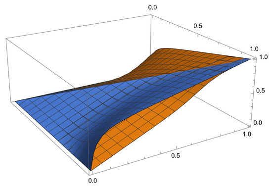
Now, in order to illustrate an intricate example, let us define the weights ${\mathrm{\Omega }}_A=({\omega }_1^A,{\omega }_2^A)$ and ${\mathrm{\Omega }}_B=({\omega }_1^B,{\omega }_2^B)$ as

$$\begin{array}{cccc}\hfill {\omega }_1^A(a_1,a_2)& =min\{2{(min\{a_1,a_2\})}^2,1\}\hfill & \hfill {\omega }_2^A(a_1,a_2)& =1-min\{2{(min\{a_1,a_2\})}^2,1\}\hfill \\ \hfill {\omega }_1^B(a_1,a_2)& =\sqrt{min\{a_1,a_2\}/2}\hfill & \hfill {\omega }_2^B(a_1,a_2)& =1-\sqrt{min\{a_1,a_2\}/2}\hfill \end{array}$$

The associated OFWA operators will be ${\mathcal{F}}_{{\mathrm{\Omega }}_A}:{[0,1]}^2\to [0,1]$ and ${\mathcal{F}}_{{\mathrm{\Omega }}_B}:{[0,1]}^2\to [0,1]$. The graph of both ${\mathcal{F}}_{{\mathrm{\Omega }}_A}$ and ${\mathcal{F}}_{{\mathrm{\Omega }}_B}$ can be found in Figure 1. In the case of small values of one of the inputs, it appears that the operator ${\mathcal{F}}_{{\mathrm{\Omega }}_A}$ is below ${\mathcal{F}}_{{\mathrm{\Omega }}_B}$, offering a more conservative viewpoint. However, in circumstances where both inputs are high, ${\mathcal{F}}_{{\mathrm{\Omega }}_A}$ becomes the most aggressive operator of the two. In particular, these operators are incomparable.

As was commented above for OWA operators, these new operators are also intermediate functions, are idempotent, and satisfy the boundary conditions. Moreover, if the weights are symmetric, then the OFWA operator is symmetric as well. Nevertheless, it is important to note that these operators are not necessarily monotone. Consequently, they do not constitute aggregation functions. Monotonicity is an essential property for aggregating functions, since higher individual values should yield a higher overall value. For this reason, Medina and Yager [17] studied some sufficient conditions on the weights $\mathrm{\Omega }$ to guarantee that the OFWA operator ${\mathcal{F}}_{\mathrm{\Omega }}$ is monotonically increasing. In particular, they introduced a family of operators based on the exponential function which are always monotonically increasing. We have provided an example to show this specific family of operators.

Example 3.

Given $k,s_1,\cdots ,s_n\in {\mathbb{R}}^{+}$ positive numbers and $m_1,\cdots ,m_n\in [0,1]$ such that $m_n\le \cdots \le m_1$, we can define the weights ${\omega }_i:{[0,1]}^n\to [0,1]$ as

$${\omega }_i(a_1,\cdots ,a_n)={\displaystyle \frac{1-m_i{e}^{-k{\left(a_1\right)}^{s_1}\cdots {\left(a_n\right)}^{s_n}}}{\mathrm{\Gamma }(a_1,\cdots ,a_n)}}$$

where $\mathrm{\Gamma }(a_1,\cdots ,a_n)=n-(m_1+\cdots +m_n)e^{-k{\left(a_1\right)}^{s_1}\cdots {\left(a_n\right)}^{s_n}}$, for all $(a_1,\cdots ,a_n)\in {[0,1]}^n$. The associated OFWA operator ${\mathcal{F}}_{{\mathrm{\Omega }}_{\gamma }}:{[0,1]}^n\to [0,1]$, with ${\mathrm{\Omega }}_{\gamma }=({\omega }_1,\cdots ,{\omega }_n)$, is increasing; see [17] [Theorem 28] for more details.

3. The Complete Lattice Structure of the OFWA Operators

This section introduces the most important results of this paper, in which the structure of the whole set of OFWA operators will be analyzed.

Theorem 1.

The set ${\mathfrak{F}}_n=\{{\mathcal{F}}_{\mathrm{\Omega }}\mid {\mathcal{F}}_{\mathrm{\Omega }}\mathit{is}\mathit{an}n‐\mathit{ary}\mathit{OFWA}\mathit{operator}\}$, together with the pairwise ordering, forms a complete lattice.

Proof. 

Since each OFWA operator lies between minimum and maximum operators, the set ${\mathfrak{F}}_n$ has a smallest and a greatest element. Hence, it is bounded. Moreover, we will focus on proving that the supremum exists and is an element of ${\mathfrak{F}}_n$ since the proof is analogous for the infimum case.

Let us consider a non-empty subset $\mathrm{\Gamma }=\{{\mathcal{F}}_{{\mathrm{\Omega }}_j}\mid j\in J\}\subseteq {\mathfrak{F}}_n$, where J is an arbitrary non-empty index set. Thus, in this case, the supremum operator $sup\left(\mathrm{\Gamma }\right):{[0,1]}^n\to [0,1]$ is defined for each $(a_1,\cdots ,a_n)\in {[0,1]}^n$ as:

$$\begin{array}{cc}\hfill sup\left(\mathrm{\Gamma }\right)(a_1,\cdots ,a_n)& =sup\{{\mathcal{F}}_{{\mathrm{\Omega }}_j}(a_1,\cdots ,a_n)\mid j\in J\}\hfill \end{array}$$

Therefore, we need to find a set of weights $W_{\mathbf{a}}=(w_{S1}^{\mathbf{a}},\cdots ,w_{Sn}^{\mathbf{a}})$ for each $\mathbf{a}=(a_1,\cdots ,a_n)\in {[0,1]}^n$ such that $F_{W_{\mathbf{a}}}\left(\mathbf{a}\right)=sup\left(\mathrm{\Gamma }\right)\left(\mathbf{a}\right)$. Given these sets, we can define the list of functional weights ${\mathrm{\Omega }}_S^{\mathrm{\Gamma }}=({\omega }_{S1},\cdots ,{\omega }_{Sn})$, where ${\omega }_{Si}(a_1,\cdots ,a_n)=w_{Si}^{\mathbf{a}}$, for all $i\in \{1,\cdots ,n\}$, and so we find that

$$sup\left(\mathrm{\Gamma }\right)={\mathcal{F}}_{{\mathrm{\Omega }}_S^{\mathrm{\Gamma }}}\in {\mathfrak{F}}_n$$

Therefore, the rest of the proof will consist in computing such sets. Since the OFWA operators are bounded by the maximum and minimum one, $a_{\rho \left(n\right)}\le sup\left(\mathrm{\Gamma }\right)(a_1,\cdots ,a_n)\le a_{\rho \left(1\right)}$. Hence, the mapping $f:[0,1]\to [0,1]$, defined as $f\left(x\right)=x{a}_{\rho \left(1\right)}+(1-x)a_{\rho \left(n\right)}$ is a continuous mapping, such that $f\left(0\right)\le sup\left(\mathrm{\Gamma }\right)(a_1,\cdots ,a_n)\le f\left(1\right)$. As a consequence of Bolzano’s Theorem, a value $c_{\mathbf{a}}\in [0,1]$ exists, such that: $f\left(c_{\mathbf{a}}\right)=sup\left(\mathrm{\Gamma }\right)(a_1,\cdots ,a_n)$. Thus, the set of weights we can consider is $W_{\mathbf{a}}=(w_{S1}^{\mathbf{a}},\cdots ,w_{Sn}^{\mathbf{a}})=(c_{\mathbf{a}},0,\cdots ,0,1-c_{\mathbf{a}})$, which finishes the proof. □

In Example 2 we mentioned that OWA operators are OFWA operators; thus, it is a subset. Moreover, when dealing with 2-ary OWA operators, this set is a chain and forms a complete sublattice of ${\mathfrak{F}}_2$.

Proposition 1.

The set of all 2-ary OWA operators is a totally ordered set.

Proof. 

Let $W=(w_1,w_2)$ and $W^{\prime }=(w_1^{\prime },w_2^{\prime })$ be two lists of weights and $F_W,F_{W^{\prime }}:{[0,1]}^2\to [0,1]$ be the associated OWA operators. Without loss of generality, we will assume that $w_1\le w_1^{\prime }$. Our goal is to show that $F_W\le F_{W^{\prime }}$ using the pointwise ordering. Since they are OWA operators, their weights add up to 1; that is, $w_1+w_2=1$, thus $w_2=1-w_1$. Therefore, we can rewrite $F_W$ as follows:

$$F_W(a_1,a_2)=w_1{a}_{\rho \left(1\right)}+w_2{a}_{\rho \left(2\right)}=w_1{a}_{\rho \left(1\right)}+(1-w_1)a_{\rho \left(2\right)}=w_1(a_{\rho \left(1\right)}-a_{\rho \left(2\right)})+a_{\rho \left(2\right)}$$

for all $(a_1,a_2)\in {[0,1]}^2$. Similarly, $F_{W^{\prime }}(a_1,a_2)=w_1^{\prime }(a_{\rho \left(1\right)}-a_{\rho \left(2\right)})+a_{\rho \left(2\right)}$. Since $w_1\le w_1^{\prime }$,

$$F_W(a_1,a_2)=w_1(a_{\rho \left(1\right)}-a_{\rho \left(2\right)})+a_{\rho \left(2\right)}\le w_1^{\prime }(a_{\rho \left(1\right)}-a_{\rho \left(2\right)})+a_{\rho \left(2\right)}=F_{W^{\prime }}(a_1,a_2)$$

for all $(a_1,a_2)\in {[0,1]}^2$. Therefore, $F_W\le F_{W^{\prime }}$. □

However, although the set of all n-ary OWA operators with $n>2$ is a partially ordered set, it does not have the same rich structure as the set of all OFWA operators. The next example will illustrate this fact.

Example 4.

Let $n>2$ and consider two lists of weights, $W=(1/2,0,\cdots ,0,1/2)$ and $W^{\prime }=(1/n,\cdots ,1/n)$. The associated OWA operators are not comparable. Indeed,

$$\begin{array}{cc}\hfill F_W(1,0,\cdots ,0)={\displaystyle \frac{1}{2}}& >{\displaystyle \frac{1}{n}}=F_W(1,0,\cdots ,0)\hfill \\ \hfill F_W(1,\cdots ,1,0)={\displaystyle \frac{1}{2}}& <{\displaystyle \frac{n-1}{n}}=F_W(1,\cdots ,1,0)\hfill \end{array}$$

Therefore, these two OWA operators are not comparable and their supremum would not be an OWA but an OFWA operator, since different values of the input correspond to different lists of weights: either W or $W^{\prime }$. Consequently, it can be deduced that the set of OWA operators does not form a sublattice of the set of OFWA operators for $n>2$.

In the proof for Theorem 1, we showed that both the supremum and infimum of a possibly infinite family of OFWA operators is also an OFWA operator. In practice, however, we will usually deal with obtaining the supremum (or infimum) of a finite number of operators. We will now show a constructive way of obtaining the supremum of OFWA operators from the weights of the elements in this setting. The infimum will be computed similarly. Let $\mathrm{\Gamma }=\{{\mathcal{F}}_{{\mathrm{\Omega }}_1},\cdots ,{\mathcal{F}}_{{\mathrm{\Omega }}_m}\}$ be a finite set of OFWA operators. The supremum operator of $\mathrm{\Gamma }$, $sup\left(\mathrm{\Gamma }\right):{[0,1]}^n\to [0,1]$, is defined as

$$\begin{array}{cc}\hfill sup\left(\mathrm{\Gamma }\right)(a_1,\cdots ,a_n)& =sup\{{\mathcal{F}}_{{\mathrm{\Omega }}_1}(a_1,\cdots ,a_n),\cdots ,{\mathcal{F}}_{{\mathrm{\Omega }}_m}(a_1,\cdots ,a_n)\}\hfill \\ \hfill & =sup\left\{\sum _{i=1}^n{\omega }_{1i}(a_1,\cdots ,a_n)a_{\rho \left(i\right)},\cdots ,\sum _{i=1}^n{\omega }_{mi}(a_1,\cdots ,a_n)a_{\rho \left(i\right)}\right\}\hfill \end{array}$$

for all $(a_1,\cdots ,a_n)\in {[0,1]}^n$, where $\rho :\{1,\cdots ,n\}\to \{1,\cdots ,n\}$ is a permutation on the index set, satisfying that $a_{\rho \left(n\right)}\le \cdots \le a_{\rho \left(1\right)}$. Since the number of values is finite and they are in the unit interval, the supremum is a maximum and so, for each $\mathbf{a}=(a_1,\cdots ,a_n)\in {[0,1]}^n$, there exists ${\mathfrak{s}}_{\mathbf{a}}\in \{1,\cdots ,m\}$, such that

$$sup\left(\mathrm{\Gamma }\right)(a_1,\cdots ,a_n)=\sum _{i=1}^n{\omega }_{{\mathfrak{s}}_{\mathbf{a}}i}(a_1,\cdots ,a_n)a_{\rho \left(i\right)}$$

Therefore, we can use these indices in order to define the set of weights ${\mathrm{\Omega }}_S^{\mathrm{\Gamma }}=({\omega }_{S1},\cdots ,{\omega }_{Sn})$ as follows

$${\omega }_{Si}(a_1,\cdots ,a_n)={\omega }_{{\mathfrak{s}}_{\mathbf{a}}i}(a_1,\cdots ,a_n)$$

for all $i\in \{1,\cdots ,n\}$ and $\mathbf{a}=(a_1,\cdots ,a_n)\in {[0,1]}^n$. From this list, we can define the OFWA operator ${\mathcal{F}}_{{\mathrm{\Omega }}_S^{\mathrm{\Gamma }}}$, which satisfies

$${\mathcal{F}}_{{\mathrm{\Omega }}_S^{\mathrm{\Gamma }}}(a_1,\cdots ,a_n)=\sum _{i=1}^n{\omega }_{{\mathfrak{s}}_{\mathbf{a}}i}(a_1,\cdots ,a_n)a_{\rho \left(i\right)}=sup\left(\mathrm{\Gamma }\right)(a_1,\cdots ,a_n)$$

for all $\mathbf{a}=(a_1,\cdots ,a_n)\in {[0,1]}^n$.

Proposition 1 stated that the set of all 2-ary OWA operators forms a chain; that is, every two elements are comparable. This is not the case for 2-ary OFWA operators. The following example shows that ${\mathfrak{F}}_2$ is not totally ordered and demonstrates how we can use the procedure mentioned above to obtain the supremum and infimum in the case of two incomparable OFWA operators.

Example 5.

Consider the OFWA operators ${\mathcal{F}}_{{\mathrm{\Omega }}_A}$ and ${\mathcal{F}}_{{\mathrm{\Omega }}_B}$ from Example 2. It can be easily shown that when $min\{a_1,a_2\}\le 0.5$, we find that ${\mathcal{F}}_{{\mathrm{\Omega }}_A}(a_1,a_2)\le {\mathcal{F}}_{{\mathrm{\Omega }}_B}(a_1,a_2)$, and when $min\{a_1,a_2\}\ge 0.5$, we obtain ${\mathcal{F}}_{{\mathrm{\Omega }}_B}(a_1,a_2)\le {\mathcal{F}}_{{\mathrm{\Omega }}_A}(a_1,a_2)$. Therefore, given $\mathrm{\Gamma }=\{{\mathcal{F}}_{{\mathrm{\Omega }}_A},{\mathcal{F}}_{{\mathrm{\Omega }}_B}\}$, we can obtain the supremum $sup\left(\mathrm{\Gamma }\right)$ and infimum $inf\left(\mathrm{\Gamma }\right)$ following the construction detailed above. For any $\mathbf{a}=(a_1,a_2)\in {[0,1]}^2$, if $min\{a_1,a_2\}\le 0.5$, we have

$$\begin{array}{cc}\hfill sup\left(\mathrm{\Gamma }\right)(a_1,a_2)& =sup\{{\mathcal{F}}_{{\mathrm{\Omega }}_A}(a_1,a_2),{\mathcal{F}}_{{\mathrm{\Omega }}_B}(a_1,a_2)\}={\mathcal{F}}_{{\mathrm{\Omega }}_B}(a_1,a_2)\hfill \\ \hfill inf\left(\mathrm{\Gamma }\right)(a_1,a_2)& =inf\{{\mathcal{F}}_{{\mathrm{\Omega }}_A}(a_1,a_2),{\mathcal{F}}_{{\mathrm{\Omega }}_B}(a_1,a_2)\}={\mathcal{F}}_{{\mathrm{\Omega }}_A}(a_1,a_2)\hfill \end{array}$$

Hence, in this case we can define ${\mathfrak{s}}_{\mathbf{a}}=B$ and ${\mathfrak{i}}_{\mathbf{a}}=A$. Otherwise, if $min\{a_1,a_2\}\ge 0.5$, we obtain that

$$\begin{array}{cc}\hfill sup\left(\mathrm{\Gamma }\right)(a_1,a_2)& =sup\{{\mathcal{F}}_{{\mathrm{\Omega }}_A}(a_1,a_2),{\mathcal{F}}_{{\mathrm{\Omega }}_B}(a_1,a_2)\}={\mathcal{F}}_{{\mathrm{\Omega }}_A}(a_1,a_2)\hfill \\ \hfill inf\left(\mathrm{\Gamma }\right)(a_1,a_2)& =inf\{{\mathcal{F}}_{{\mathrm{\Omega }}_A}(a_1,a_2),{\mathcal{F}}_{{\mathrm{\Omega }}_B}(a_1,a_2)\}={\mathcal{F}}_{{\mathrm{\Omega }}_B}(a_1,a_2)\hfill \end{array}$$

Thus, we define ${\mathfrak{s}}_{\mathbf{a}}=A$ and ${\mathfrak{i}}_{\mathbf{a}}=B$. As a result, we can define two OFWA operators ${\mathcal{F}}_{{\mathrm{\Omega }}_S^{\mathrm{\Gamma }}}$ and ${\mathcal{F}}_{{\mathrm{\Omega }}_I^{\mathrm{\Gamma }}}$, where ${\mathrm{\Omega }}_S^{\mathrm{\Gamma }}=({\omega }_1^{{\mathfrak{s}}_{\mathbf{a}}},{\omega }_2^{{\mathfrak{s}}_{\mathbf{a}}})$ and ${\mathrm{\Omega }}_I^{\mathrm{\Gamma }}=({\omega }_1^{{\mathfrak{i}}_{\mathbf{a}}},{\omega }_2^{{\mathfrak{i}}_{\mathbf{a}}})$ are defined as

$$\begin{array}{cc}\hfill {\omega }_i^{{\mathfrak{s}}_{\mathbf{a}}}(a_1,a_2)& =\left\{\begin{array}{cc}{\omega }_i^B(a_1,a_2)\hfill & \mathit{if}min\{a_1,a_2\}\le 0.5\hfill \\ {\omega }_i^A(a_1,a_2)\hfill & \mathit{otherwise}\hfill \end{array}\right.\hfill \\ \hfill {\omega }_i^{{\mathfrak{i}}_{\mathbf{a}}}(a_1,a_2)& =\left\{\begin{array}{cc}{\omega }_i^A(a_1,a_2)\hfill & \mathit{if}min\{a_1,a_2\}\le 0.5\hfill \\ {\omega }_i^B(a_1,a_2)\hfill & \mathit{otherwise}\hfill \end{array}\right.\hfill \end{array}$$

for all $(a_1,a_2)\in {[0,1]}^2$ and $i\in \{1,2\}$. Therefore, we find that

$$sup\left(\mathrm{\Gamma }\right)={\mathcal{F}}_{{\mathrm{\Omega }}_S^{\mathrm{\Gamma }}},inf\left(\mathrm{\Gamma }\right)={\mathcal{F}}_{{\mathrm{\Omega }}_I^{\mathrm{\Gamma }}}$$

The OFWA operator $F_{{\mathrm{\Omega }}_S^{\mathrm{\Gamma }}}$ was constructed with an aggressive point of view in mind, whereas ${\mathcal{F}}_{{\mathrm{\Omega }}_I^{\mathrm{\Gamma }}}$ corresponds to a conservative viewpoint. Hence, ${\mathcal{F}}_{{\mathrm{\Omega }}_I^{\mathrm{\Gamma }}}\le {\mathcal{F}}_{{\mathrm{\Omega }}_S^{\mathrm{\Gamma }}}$ and so

$$sup\left(\{{\mathcal{F}}_{{\mathrm{\Omega }}_S^{\mathrm{\Gamma }}},{\mathcal{F}}_{{\mathrm{\Omega }}_I^{\mathrm{\Gamma }}}\}\right)={\mathcal{F}}_{{\mathrm{\Omega }}_S^{\mathrm{\Gamma }}},inf\left(\{{\mathcal{F}}_{{\mathrm{\Omega }}_S^{\mathrm{\Gamma }}},{\mathcal{F}}_{{\mathrm{\Omega }}_I^{\mathrm{\Gamma }}}\}\right)={\mathcal{F}}_{{\mathrm{\Omega }}_I^{\mathrm{\Gamma }}}$$

In addition, based on Theorem 1, we can reach the conclusion that the set of OFWA operators forms a complete lattice, with top and bottom elements being the maximum and minimum operators, respectively. This is an important property, which has several interesting aspects. For example, in order to aggregate the different OWA or OFWA, operators considered the input of diverse experts, who expressed either an aggressive or conservative point of view. In the following example, we expose a scenario where two OFWA operators are aggregated, yielding two other OFWA operators: one conservative and the other aggressive.

Example 6.

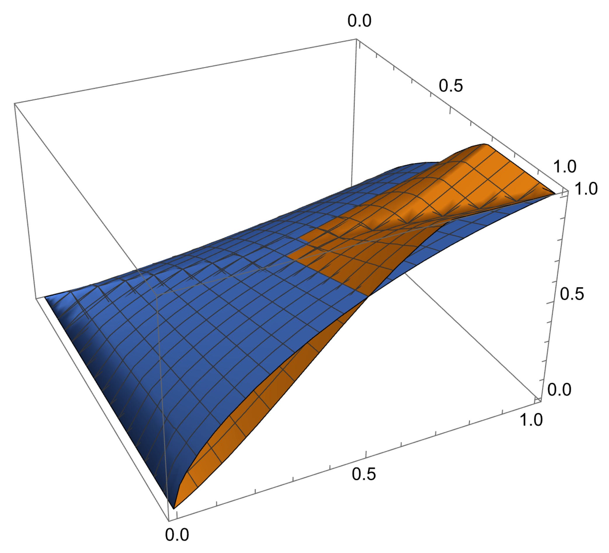
Consider two particular cases of the OFWA operators presented in Example 3, ${\mathcal{F}}_{\mathrm{\Omega }}:{[0,1]}^2\to [0,1]$ and ${\mathcal{F}}_{{\mathrm{\Omega }}^{\prime }}:{[0,1]}^2\to [0,1]$, defined for all $a_1,a_2\in [0,1]$ as

$$\begin{array}{cc}\hfill {\mathcal{F}}_{\mathrm{\Omega }}(a_1,a_2)& ={\displaystyle \frac{1-e^{-10a_1{\left(a_2\right)}^{10}}}{\mathrm{\Gamma }(a_1,a_2)}}{a}_{\rho \left(1\right)}+{\displaystyle \frac{1-0.5e^{-10a_1{\left(a_2\right)}^{10}}}{\mathrm{\Gamma }(a_1,a_2)}}{a}_{\rho \left(2\right)}\hfill \\ \hfill {\mathcal{F}}_{{\mathrm{\Omega }}^{\prime }}(a_1,a_2)& ={\displaystyle \frac{1-e^{-10{\left(a_1\right)}^{10}{a}_2}}{{\mathrm{\Gamma }}^{\prime }(a_1,a_2)}}{a}_{\rho \left(1\right)}+{\displaystyle \frac{1-0.5e^{-10{\left(a_1\right)}^{10}{a}_2}}{{\mathrm{\Gamma }}^{\prime }(a_1,a_2)}}{a}_{\rho \left(2\right)}\hfill \end{array}$$

where $\mathrm{\Gamma }(a_1,a_2)=2-1.5e^{-10a_1{\left(a_2\right)}^{10}}$ and ${\mathrm{\Gamma }}^{\prime }(a_1,a_2)=2-1.5e^{-10{\left(a_1\right)}^{10}{a}_2}$. Figure 2 shows a graph of both these operators.

In a decision-making problem with two inputs, we have two experts, one of them wanted to favor the second input (${\mathcal{F}}_{\mathrm{\Omega }}$), whereas the other considered the first input to be more reliable (${\mathcal{F}}_{{\mathrm{\Omega }}^{\prime }}$). In order to account for both of the experts’ opinions, we might use the aggressive point of view, using the supremum of the two, or the conservative point of view, via the infimum.

It is clear that ${\mathcal{F}}_{\mathrm{\Omega }}(a_1,a_2)={\mathcal{F}}_{{\mathrm{\Omega }}^{\prime }}(a_2,a_1)$, for all $(a_1,a_2)\in {[0,1]}^2$, so to compare the two operators we can focus on the values $(a_1,a_2)\in {[0,1]}^2$, such that $a_2\le a_1$. We wish to show that ${\mathcal{F}}_{\mathrm{\Omega }}(a_1,a_2)\le {\mathcal{F}}_{{\mathrm{\Omega }}^{\prime }}(a_1,a_2)$, for all $(a_1,a_2)\in {[0,1]}^2$, such that $a_2\le a_1$. Since $\mathrm{\Gamma }(a_1,a_2)$ and ${\mathrm{\Gamma }}^{\prime }(a_1,a_2)$ are both positive, we will focus on the sign of $\mathrm{\Gamma }(a_1,a_2){\mathrm{\Gamma }}^{\prime }(a_1,a_2)({\mathcal{F}}_{\mathrm{\Omega }}(a_1,a_2)-{\mathcal{F}}_{{\mathrm{\Omega }}^{\prime }}(a_1,a_2))$. From simple calculations, this quantity is

$$\begin{array}{c}\hfill 0.5(a_1-a_2)\left(e^{-10a_1^{10}{a}_2}-e^{-10a_1{a}_2^{10}}\right)\end{array}$$

It is clear that, if $a_2\le a_1$, then $a_1-a_2$ is positive and $e^{-10a_1^{10}{a}_2}-e^{-10a_1{a}_2^{10}}$ is negative, that is, ${\mathcal{F}}_{\mathrm{\Omega }}(a_1,a_2)\le {\mathcal{F}}_{{\mathrm{\Omega }}^{\prime }}(a_1,a_2)$. Therefore,

$$sup\{{\mathcal{F}}_{\mathrm{\Omega }},{\mathcal{F}}_{{\mathrm{\Omega }}^{\prime }}\}(a_1,a_2)=\left\{\begin{array}{cc}{\mathcal{F}}_{\mathrm{\Omega }}(a_1,a_2)\hfill & \mathrm{if}{a}_1\le a_2\hfill \\ {\mathcal{F}}_{{\mathrm{\Omega }}^{\prime }}(a_1,a_2)\hfill & \mathrm{if}{a}_2\le a_1\hfill \end{array}\right.$$

and

$$inf\{{\mathcal{F}}_{\mathrm{\Omega }},{\mathcal{F}}_{{\mathrm{\Omega }}^{\prime }}\}(a_1,a_2)=\left\{\begin{array}{cc}{\mathcal{F}}_{{\mathrm{\Omega }}^{\prime }}(a_1,a_2)\hfill & \mathrm{if}{a}_1\le a_2\hfill \\ {\mathcal{F}}_{\mathrm{\Omega }}(a_1,a_2)\hfill & \mathrm{if}{a}_2\le a_1\hfill \end{array}\right.$$

The previous example can be extended to any decision-making problem with an arbitrary number of experts and family of OFWA operators. The following section presents a practical example.

4. A Practical Example

In this section, a practical example is presented in which two experts propose two different ways of aggregating the information given by the inverters of a photovoltaic facility in order to detect changes in the energy production. This example is based on the problem considered in [19].

The photovoltaic facility consists of seven inverters (${\mathrm{I}}_1$ through ${\mathrm{I}}_7$), each generating a value within $[0,1]$ that represents its performance at any given moment. To determine the overall output of the facility, the individual values are aggregated, making use of an OWA or OFWA operator. Expert 1 suggest that the two highest and two lowest values should be discarded and the average of the remaining three should be calculated. Therefore, we would use the OWA associated with the list of weights $W=(0,0,1/3,1/3,1/3,0,0)$; that is, the operator $F_W:{[0,1]}^7\to [0,1]$, defined as

$$F_W(a_1,a_2,a_3,a_4,a_5,a_6,a_7)={\displaystyle \frac{a_{\rho \left(3\right)}+a_{\rho \left(4\right)}+a_{\rho \left(5\right)}}{3}}$$

where $\rho :\{1,\cdots ,n\}\to \{1,\cdots ,n\}$ is a permutation on the index set, satisfying that $a_{\rho \left(n\right)}\le \cdots \le a_{\rho \left(1\right)}$.

However, Expert 2 has noticed that the inverters ${\mathrm{I}}_6$ and ${\mathrm{I}}_7$ are very reliable when outputting low values. Whenever both their outputs are below $0.4$, Expert 2 recommends not excluding the lower values and averaging the remainder. Moreover, the inverters ${\mathrm{I}}_1$ and ${\mathrm{I}}_2$ also seem to be accurate when high values are involved. Consequently, they indicate that the higher values should not be omitted when their outputs are above $0.7$.

To build an OFWA operator taking into account the instructions from Expert 2, we need to consider two regions in ${[0,1]}^7$: when the outputs from ${\mathrm{I}}_6$ and ${\mathrm{I}}_7$ are below $0.4$, the set $A_L={[0,1]}^5\times {[0,0.4]}^2$, and when the outputs from ${\mathrm{I}}_1$ and ${\mathrm{I}}_2$ are over $0.7$, the set $A_H={[0.7,1]}^2\times {[0,1]}^5$. From these, we can define the characteristic regions for the OFWA operator.

• If the outputs are in both $A_L$ and $A_H$, we take all the values into account and average them; that is, we use the weights $(1/7,1/7,1/7,1/7,1/7,1/7,1/7)$. The corresponding region is

  $$A_1=A_L\cap A_H={[0.7,1]}^2\times {[0,1]}^3\times {[0,0.4]}^2$$
• If the output is in $A_H$ but not in $A_L$, we omit the two lowest values and average the rest using the weights $(1/5,1/5,1/5,1/5,1/5,0,0)$. The corresponding region is

  $$A_2=A_H\setminus A_L={[0.7,1]}^2\times {[0,1]}^3\times {(0.4,1]}^2$$
• If the output is in $A_L$ but not in $A_H$, we leave out the two highest values and average the rest with the weights $(0,0,1/5,1/5,1/5,1/5,1/5)$. The corresponding region is

  $$A_3=A_L\setminus A_H={[0,0.7)}^2\times {[0,1]}^3\times {[0,0.4]}^2$$
• If the output is neither in $A_L$ nor in $A_H$, we only take into account the middle three values and obtain their average; that is, we use the weights $(0,0,1/3,1/3,1/3,0,0)$. The corresponding region is

  $$A_4={[0,1]}^7\setminus (A_L\cup A_H)={[0,0.7)}^2\times {[0,1]}^3\times {(0.4,1]}^2$$

The resulting OFWA operator ${\mathcal{F}}_{\mathrm{\Omega }}:{[0,1]}^7\to [0,1]$ will be defined by the weights

$$\begin{array}{cc}\hfill {\omega }_1\left(\mathbf{a}\right)={\omega }_2\left(\mathbf{a}\right)& =\left\{\begin{array}{cc}1/7\hfill & \mathrm{if}\mathbf{a}\in A_1\hfill \\ 1/5\hfill & \mathrm{if}\mathbf{a}\in A_2\hfill \\ 0\hfill & \mathrm{if}\mathbf{a}\in A_3\hfill \\ 0\hfill & \mathrm{if}\mathbf{a}\in A_4\hfill \end{array}\right.\hfill \\ \hfill {\omega }_3\left(\mathbf{a}\right)={\omega }_4\left(\mathbf{a}\right)={\omega }_5\left(\mathbf{a}\right)& =\left\{\begin{array}{cc}1/7\hfill & \mathrm{if}\mathbf{a}\in A_1\hfill \\ 1/5\hfill & \mathrm{if}\mathbf{a}\in A_2\hfill \\ 1/5\hfill & \mathrm{if}\mathbf{a}\in A_3\hfill \\ 1/3\hfill & \mathrm{if}\mathbf{a}\in A_4\hfill \end{array}\right.\hfill \\ \hfill {\omega }_6\left(\mathbf{a}\right)={\omega }_7\left(\mathbf{a}\right)& =\left\{\begin{array}{cc}1/7\hfill & \mathrm{if}\mathbf{a}\in A_1\hfill \\ 0\hfill & \mathrm{if}\mathbf{a}\in A_2\hfill \\ 1/5\hfill & \mathrm{if}\mathbf{a}\in A_3\hfill \\ 0\hfill & \mathrm{if}\mathbf{a}\in A_4\hfill \end{array}\right.\hfill \end{array}$$

The OWA operator of Expert 1 is clearly less complex than the OFWA operator proposed by Expert 2. However, the OFWA operator allows for greater flexibility, enabling the user to take into account important external factors. Nonetheless, we want to factor in the opinion of both experts, obtaining an overall conservative or aggressive output.

Hence, we can apply the results in Section 3 to compute the supremum (aggressive) and infimum (conservative) of both operators. Clearly, this must be done by region. For example, if we take into account region $A_2$, we can see that the OWA operator $F_W$ averages the three middle values, whereas ${\mathcal{F}}_{\mathrm{\Omega }}$ also considers the two higher values. Since using $F_{\mathrm{\Omega }}$ means we are shifting the weights of $F_W$ towards higher values, it is natural to think that the resulting output will be higher. Indeed,

$$\begin{array}{cc}\hfill F_W(a_1,\cdots ,a_7)& ={\displaystyle \frac{1}{3}}{a}_{\rho \left(3\right)}+{\displaystyle \frac{1}{3}}{a}_{\rho \left(4\right)}+{\displaystyle \frac{1}{3}}{a}_{\rho \left(5\right)}\hfill \\ \hfill & =\left({\displaystyle \frac{2}{15}}{a}_{\rho \left(3\right)}+{\displaystyle \frac{1}{15}}{a}_{\rho \left(4\right)}\right)+\left({\displaystyle \frac{1}{15}}{a}_{\rho \left(4\right)}+{\displaystyle \frac{2}{15}}{a}_{\rho \left(5\right)}\right)+{\displaystyle \frac{1}{5}}{a}_{\rho \left(3\right)}+{\displaystyle \frac{1}{5}}{a}_{\rho \left(4\right)}+{\displaystyle \frac{1}{5}}{a}_{\rho \left(5\right)}\hfill \\ \hfill (\ast )& \le \left({\displaystyle \frac{2}{15}}{a}_{\rho \left(1\right)}+{\displaystyle \frac{1}{15}}{a}_{\rho \left(1\right)}\right)+\left({\displaystyle \frac{1}{15}}{a}_{\rho \left(2\right)}+{\displaystyle \frac{2}{15}}{a}_{\rho \left(2\right)}\right)+{\displaystyle \frac{1}{5}}{a}_{\rho \left(3\right)}+{\displaystyle \frac{1}{5}}{a}_{\rho \left(4\right)}+{\displaystyle \frac{1}{5}}{a}_{\rho \left(5\right)}\hfill \\ \hfill & ={\displaystyle \frac{1}{5}}{a}_{\rho \left(1\right)}+{\displaystyle \frac{1}{5}}{a}_{\rho \left(2\right)}+{\displaystyle \frac{1}{5}}{a}_{\rho \left(3\right)}+{\displaystyle \frac{1}{5}}{a}_{\rho \left(4\right)}+{\displaystyle \frac{1}{5}}{a}_{\rho \left(5\right)}\hfill \\ \hfill & ={\mathcal{F}}_{\mathrm{\Omega }}(a_1,\cdots ,a_7)\hfill \end{array}$$

where in $(\ast )$, we have used the fact that $a_{\rho \left(5\right)}\le a_{\rho \left(4\right)}\le a_{\rho \left(3\right)}\le a_{\rho \left(2\right)}\le a_{\rho \left(1\right)}$. Therefore, the supremum in this region will be ${\mathcal{F}}_{\mathrm{\Omega }}$ and the infimum $F_W$. This must be repeated for the rest of the regions. Only in region $A_1$ do both operators remain incomparable, meaning that subregions must be divided to obtain the final supremum and infimum operators. This division is given by

$$\begin{array}{cc}\hfill A_{11}& =\left\{(a_1,a_2,a_3,a_4,a_5,a_6,a_7)\in {[0,1]}^7\mid a_1+a_2+a_6+a_7>2{\displaystyle \frac{a_3+a_4+a_5}{5}}\right\}\hfill \\ \hfill A_{12}& =\left\{(a_1,a_2,a_3,a_4,a_5,a_6,a_7)\in {[0,1]}^7\mid a_1+a_2+a_6+a_7\le 2{\displaystyle \frac{a_3+a_4+a_5}{5}}\right\}\hfill \end{array}$$

Finally, the supremum and infimum operators are the following:

$$\begin{array}{cc}\hfill sup\{F_W,{\mathcal{F}}_{\mathrm{\Omega }}\}\left(\mathbf{a}\right)& =\left\{\begin{array}{cc}{\mathcal{F}}_{\mathrm{\Omega }}\left(\mathbf{a}\right)\hfill & \mathrm{if}\mathbf{a}\in A_{11}\hfill \\ F_W\left(\mathbf{a}\right)\hfill & \mathrm{if}\mathbf{a}\in A_{12}\hfill \\ {\mathcal{F}}_{\mathrm{\Omega }}\left(\mathbf{a}\right)\hfill & \mathrm{if}\mathbf{a}\in A_2\hfill \\ F_W\left(\mathbf{a}\right)\hfill & \mathrm{if}\mathbf{a}\in A_3\hfill \\ {\mathcal{F}}_{\mathrm{\Omega }}\left(\mathbf{a}\right)=F_W\left(\mathbf{a}\right)\hfill & \mathrm{if}\mathbf{a}\in A_4\hfill \end{array}\right.\hfill \\ \hfill inf\{F_W,{\mathcal{F}}_{\mathrm{\Omega }}\}\left(\mathbf{a}\right)& =\left\{\begin{array}{cc}{F}_W\left(\mathbf{a}\right)\hfill & \mathrm{if}\mathbf{a}\in A_{11}\hfill \\ {\mathcal{F}}_{\mathrm{\Omega }}\left(\mathbf{a}\right)\hfill & \mathrm{if}\mathbf{a}\in A_{12}\hfill \\ F_W\left(\mathbf{a}\right)\hfill & \mathrm{if}\mathbf{a}\in A_2\hfill \\ {\mathcal{F}}_{\mathrm{\Omega }}\left(\mathbf{a}\right)\hfill & \mathrm{if}\mathbf{a}\in A_3\hfill \\ {\mathcal{F}}_{\mathrm{\Omega }}\left(\mathbf{a}\right)=F_W\left(\mathbf{a}\right)\hfill & \mathrm{if}\mathbf{a}\in A_4\hfill \end{array}\right.\hfill \end{array}$$

Alternatively,

$${\omega }_{S1}\left(\mathbf{a}\right)={\omega }_{S2}\left(\mathbf{a}\right)=\left\{\begin{array}{cc}1/7\hfill & \mathrm{if}\mathbf{a}\in A_{11}\hfill \\ 0\hfill & \mathrm{if}\mathbf{a}\in A_{12}\hfill \\ 1/5\hfill & \mathrm{if}\mathbf{a}\in A_2\hfill \\ 0\hfill & \mathrm{if}\mathbf{a}\in A_3\hfill \\ 0\hfill & \mathrm{if}\mathbf{a}\in A_4\hfill \end{array}\right.\hspace{1em}\hspace{1em}{\omega }_{I1}\left(\mathbf{a}\right)={\omega }_{I2}\left(\mathbf{a}\right)=\left\{\begin{array}{cc}0\hfill & \mathrm{if}\mathbf{a}\in A_{11}\hfill \\ 1/7\hfill & \mathrm{if}\mathbf{a}\in A_{12}\hfill \\ 0\hfill & \mathrm{if}\mathbf{a}\in A_2\hfill \\ 0\hfill & \mathrm{if}\mathbf{a}\in A_3\hfill \\ 0\hfill & \mathrm{if}\mathbf{a}\in A_4\hfill \end{array}\right.$$

$$\begin{array}{c}{\omega }_{S3}\left(\mathbf{a}\right)=\hfill \\ {\omega }_{S4}\left(\mathbf{a}\right)={\omega }_{S5}\left(\mathbf{a}\right)=\hfill \end{array}\left\{\begin{array}{cc}1/7\hfill & \mathrm{if}\mathbf{a}\in A_{11}\hfill \\ 1/3\hfill & \mathrm{if}\mathbf{a}\in A_{12}\hfill \\ 1/5\hfill & \mathrm{if}\mathbf{a}\in A_2\hfill \\ 1/3\hfill & \mathrm{if}\mathbf{a}\in A_3\hfill \\ 1/3\hfill & \mathrm{if}\mathbf{a}\in A_4\hfill \end{array}\right.\hspace{1em}\hspace{1em}\begin{array}{c}{\omega }_{I3}\left(\mathbf{a}\right)=\hfill \\ {\omega }_{I4}\left(\mathbf{a}\right)={\omega }_{I5}\left(\mathbf{a}\right)=\hfill \end{array}\left\{\begin{array}{cc}1/3\hfill & \mathrm{if}\mathbf{a}\in A_{11}\hfill \\ 1/7\hfill & \mathrm{if}\mathbf{a}\in A_{12}\hfill \\ 1/3\hfill & \mathrm{if}\mathbf{a}\in A_2\hfill \\ 1/5\hfill & \mathrm{if}\mathbf{a}\in A_3\hfill \\ 1/3\hfill & \mathrm{if}\mathbf{a}\in A_4\hfill \end{array}\right.$$

$${\omega }_{S6}\left(\mathbf{a}\right)={\omega }_{S7}\left(\mathbf{a}\right)=\left\{\begin{array}{cc}1/7\hfill & \mathrm{if}\mathbf{a}\in A_{11}\hfill \\ 0\hfill & \mathrm{if}\mathbf{a}\in A_{12}\hfill \\ 0\hfill & \mathrm{if}\mathbf{a}\in A_2\hfill \\ 0\hfill & \mathrm{if}\mathbf{a}\in A_3\hfill \\ 0\hfill & \mathrm{if}\mathbf{a}\in A_4\hfill \end{array}\right.\hspace{1em}\hspace{1em}{\omega }_{I6}\left(\mathbf{a}\right)={\omega }_{I7}\left(\mathbf{a}\right)=\left\{\begin{array}{cc}0\hfill & \mathrm{if}\mathbf{a}\in A_{11}\hfill \\ 1/7\hfill & \mathrm{if}\mathbf{a}\in A_{12}\hfill \\ 0\hfill & \mathrm{if}\mathbf{a}\in A_2\hfill \\ 1/5\hfill & \mathrm{if}\mathbf{a}\in A_3\hfill \\ 0\hfill & \mathrm{if}\mathbf{a}\in A_4\hfill \end{array}\right.$$

Therefore, $sup\{F_W,{\mathcal{F}}_{\mathrm{\Omega }}\}={\mathcal{F}}_{{\mathrm{\Omega }}_S}$ and $inf\{F_W,{\mathcal{F}}_{\mathrm{\Omega }}\}={\mathcal{F}}_{{\mathrm{\Omega }}_I}$, where ${\mathrm{\Omega }}_S=({\omega }_{S1},{\omega }_{S2},{\omega }_{S3},{\omega }_{S4},{\omega }_{S5},{\omega }_{S6},{\omega }_{S7})$ and ${\mathrm{\Omega }}_I=({\omega }_{I1},{\omega }_{I2},{\omega }_{I3},{\omega }_{I4},{\omega }_{I5},{\omega }_{I6},{\omega }_{I7})$.

5. Conclusions and Future Work

This paper has presented fundamental results in order to aggregate OFWA operators. In particular, we have proven that the whole set of OFWA operators forms a complete lattice, unlike the OWA operators, whose relationship only provides a lattice structure when 2-ary OWA operators are considered. A procedure to compute the supremum and infimum of finite sets of OFWA operators has also been introduced. Different examples have illustrated these results and different scenarios which are of particular interest. In particular, a real case of solar photovoltaic facility management has also been considered, in which we are able to combine the knowledge of two different experts for fault detection.

In the future, other operators that can be used to aggregate OFWA operators will be studied. Moreover, more families of OFWA operators will be analyzed and sufficient conditions to ensure the usual monotonicity or other variants, such as directional monotonicity [20], will be investigated. Furthermore, some extensions following the philosophies of weighted and linguistic OWA operators [21,22,23] will also be examined.

References

- Haloui, D.; Oufaska, K.; Oudani, M.; Yassini, K.E.; Belhadi, A.; Kamble, S. Sustainable urban farming using a two-phase multi-objective and multi-criteria decision-making approach. Int. Trans. Oper. Res. 2025, 32, 769–801. [Google Scholar] [CrossRef]
- Kim, J.H.; Kim, J.; Park, J.; Kim, C.; Jhang, J.; King, B. When chatGPT gives incorrect answers: The impact of inaccurate information by generative ai on tourism decision-making. J. Travel Res. 2025, 64, 51–73. [Google Scholar] [CrossRef]
- Sadana, U.; Chenreddy, A.; Delage, E.; Forel, A.; Frejinger, E.; Vidal, T. A survey of contextual optimization methods for decision-making under uncertainty. Eur. J. Oper. Res. 2025, 320, 271–289. [Google Scholar] [CrossRef]
- Bellman, R.E.; Zadeh, L.A. Decision-making in a fuzzy environment. Manag. Sci. 1970, 17, B‐141–B‐164. [Google Scholar] [CrossRef]
- Chacón-Gómez, F.; Cornejo, M.E.; Medina, J. Decision making in fuzzy rough set theory. Mathematics 2023, 11, 4187. [Google Scholar] [CrossRef]
- Chen, Q.; Zhao, Q.; Zou, Z.; Qian, Q.; Zhou, J.; Yuan, R. A novel air combat target threat assessment method based on three-way decision and game theory under multi-criteria decision-making environment. Expert Syst. Appl. 2025, 259, 125322. [Google Scholar] [CrossRef]
- Su, J.; Liu, H.; Chen, Y.; Zhang, N.; Li, J. A novel multi-criteria decision making method to evaluate green innovation ecosystem resilience. Eng. Appl. Artif. Intell. 2025, 139, 109528. [Google Scholar] [CrossRef]
- Martínez-Gutiérrez, A.; Sánchez-Calleja, I.; Ferrero-Guillén, R.; Díez-González, J. On the selection of aircraft-engine pairs for medium-haul low-cost carriers operations. J. Air Transp. Manag. 2024, 120, 102657. [Google Scholar] [CrossRef]
- Yager, R.R. On ordered weighted averaging aggregation operators in multicriteria decision-making. IEEE Trans. Syst. Man Cybern. 1988, 18, 183–190. [Google Scholar] [CrossRef]
- Lizasoain, I.; Moreno, C. OWA operators defined on complete lattices. Fuzzy Sets Syst. 2013, 224, 36–52. [Google Scholar] [CrossRef]
- Kishor, A.; Singh, A.K.; Pal, N.R. Orness measure of OWA operators: A new approach. IEEE Trans. Fuzzy Syst. 2014, 22, 1039–1045. [Google Scholar] [CrossRef]
- Yager, R.R. Families of OWA operators. Fuzzy Sets Syst. 1993, 59, 125–148. [Google Scholar] [CrossRef]
- Baz, J.; García-Zamora, D.; Díaz, I.; Montes, S.; Martínez, L. Flexible-dimensional L-statistic for mean estimation of symmetric distributions. Stat. Pap. 2024, 65, 4001–4024. [Google Scholar] [CrossRef]
- Al-Amidie, M.; Alzubaidi, L.; Islam, M.A.; Anderson, D.T. Enhancing sensor data imputation: OWA-based model aggregation for missing values. Future Internet 2024, 16, 193. [Google Scholar] [CrossRef]
- Gong, C.; Siraj, S.; Yu, L.; Fu, L. A generalized form of the distance-induced OWA operators–Demonstrating its use for evaluation indicator system in china. Expert Syst. Appl. 2024, 247, 123257. [Google Scholar] [CrossRef]
- Rachwał, A.; Karczmarek, P.; Rachwał, A. Smooth ordered weighted averaging operators. Inf. Sci. 2025, 686, 121343. [Google Scholar] [CrossRef]
- Medina, J.; Yager, R.R. OWA operators with functional weights. Fuzzy Sets Syst. 2021, 414, 38–56. [Google Scholar] [CrossRef]
- Davey, B.; Priestley, H. Introduction to Lattices and Order, 2nd ed.; Cambridge University Press: Cambridge, UK, 2002. [Google Scholar]
- Aragón, R.G.; Cornejo, M.E.; Medina, J.; Moreno-García, J.; Ramírez-Poussa, E. Decision support system for photovoltaic fault detection avoiding meteorological conditions. Int. J. Inf. Technol. Decis. Mak. 2022, 21, 911–932. [Google Scholar] [CrossRef]
- Marco-Detchart, C.; Bustince, H.; Fernandez, J.; Mesiar, R.; Lafuente, J.; Barrenechea, E.; Pintor, J. Ordered directional monotonicity in the construction of edge detectors. Fuzzy Sets Syst. 2021, 421, 111–132. [Google Scholar] [CrossRef]
- Herrera, F.; Herrera-Viedma, E.; Verdegay, J. Direct approach processes in group decision making using linguistic owa operators. Fuzzy Sets Syst. 1996, 79, 175–190. [Google Scholar] [CrossRef]
- Serrano-Guerrero, J.; Bani-Doumi, M.; Romero, F.P.; Olivas, J.A. A 2-tuple fuzzy linguistic model for recommending health care services grounded on aspect-based sentiment analysis. Expert Syst. Appl. 2024, 238, 122340. [Google Scholar] [CrossRef]
- Torra, V. Andness directedness for operators of the owa and wowa families. Fuzzy Sets Syst. 2021, 414, 28–37. [Google Scholar] [CrossRef]
Disclaimer/Publisher’s Note: The statements, opinions and data contained in all publications are solely those of the individual author(s) and contributor(s) and not of MDPI and/or the editor(s). MDPI and/or the editor(s) disclaim responsibility for any injury to people or property resulting from any ideas, methods, instructions or products referred to in the content. |
© 2025 by the authors. Licensee MDPI, Basel, Switzerland. This article is an open access article distributed under the terms and conditions of the Creative Commons Attribution (CC BY) license (https://creativecommons.org/licenses/by/4.0/).