Integral-Based Memory Event-Triggered Controller Design for Uncertain Neural Networks with Control Input Missing

Abstract

In this paper, the controller design problem for uncertain neural networks (NNs) with control input missing is addressed under an event-triggered (ET) scheme. First, under the zero-input method, the closed-loop system is modeled as a switched system which includes a stable subsystem and an unstable subsystem. Next, a novel integral-based memory event-triggered (IMET) scheme is designed, which can prevent Zeno behavior. The proposed IMET scheme is designed over a specified memory interval; thus, it can make full use of the historical state information, thereby reducing the adverse impact caused by packet dropouts. Then, with the analysis method of switched systems, a piecewise time-dependent Lyapunov functional is designed, and low conservative conditions are derived to ensure the exponential stability of the switched closed-loop system. Meanwhile, the constraints on the packet loss rate and the average dwell time are established. Moreover, the design of the controller gain is also given. Finally, the feasibility of IMET is verified using an example.

1. Introduction

Due to their powerful adaptability, self-organization, and self-learning abilities, neural networks (NNs) have become a research hotspot for many scholars [1,2,3,4]. However, in the implementation of NNs, uncertainties are often encountered because of inaccurate modeling or environmental noise, which can degrade system performance and further lead to system instability [5,6,7]. In addition, on account of unreliable communication channels and limited bandwidth, the control signal may not reach the receiving terminal successfully. Hence, data packet dropout is an inevitable problem for the control of NNs. When packet dropout occurs from the controller to the actuator channel, it is referred ti as missing control input [8]. This phenomenon is inevitable due to actuator failure, intermittent controller unavailability, and other reasons. Generally, there are two methods to cope with this problem. One is the hold-input method [9,10]; that is, when the controller signal is lost, the latest control signal is taken as the input of the actuator. The other is the zero-input method [11,12,13,14]; that is, when the control signal is lost, the input of the actuator is set to zero, then the controlled system can be converted to a switched system. Promising results on systems with packet dropout have been achieved. For example, based on the zero-input method, robust synchronization for uncertainty delayed NNs with control packet dropout was implemented under sampling control in [12]. For fuzzy system with packet dropouts, refs. [13,14] studied robust $H_{\infty }$ control and exponential stabilization using the zero-input method under sampling control, respectively. It should be noted that although related research on neural networks incorporating these two network-induced phenomena has achieved certain results, there remains significant room for improvement.

On the other hand, networked control methods have attracted considerable attention in recent decades. As is well known, traditional time-triggered control methods will generate redundant data and therefore lead to over-occupation of limited communication bandwidth and blockage of information channels. It has been proved in [15] that the integration of an event-triggered scheme into the controller can effectively reduce the number of control task executions. Thereafter, ET control has attracted increasing attention from scholars [16,17,18,19,20]. The sampling of ET control is carried out only when a preset event is triggered; that is, the system will transmit information only as needed. In this way, the waste of network resources can be reduced while guaranteeing the expected performance. Among the existing ET schemes, the periodic event-triggered (PET) scheme is a classic one, in which the preset triggering condition is monitored periodically [21,22]. It can ensure that the interval between two adjacent triggers is greater than zero, so it can automatically avoid the emergence of Zeno phenomena. Based on the PET scheme, a novel ET scheme called the memory-based event-triggered (MET) scheme was devised in [23]. The MET scheme comprehensively utilizes the difference between historically transmitted data and the currently sampled data to design the triggering condition [24,25,26,27]. What needs to be pointed out is that most existing METs use the discrete mean value of a certain number of historically sampled or triggered data. However, if packet dropouts occur, some sampled data are partial, or all missing, then the effect of the MET scheme using a discrete mean value will be reduced. However, if the continuous mean value—that is, the integral over a past continuous interval—is employed to design the triggering condition, even if some sampled data are lost, the integral can still address the issue related to packet dropout due to the good property of the integral. In this way, both higher control performance and fewer triggering times can be achieved.

Enlightened by the above thoughts, this paper will investigate the stabilization of NNs with uncertainty and control input missing by designing an ET scheme. The contributions of this paper can be summarized as follows:

(1) To deal with the impact of packet dropout, a novel MET scheme, named IMET, is devised, which introduces an integral of the system state over a specified memory interval. The proposed IMET scheme can not only make use of the historical state information but also alleviate the effects of packet dropout and exclude the occurrence of Zeno phenomena.

(2) Under the proposed IMET scheme, the uncertain NN with control input missing is modeled by a switched system on the basis of the zero-input method. Then, a piecewise time-dependent Lyapunov functional consisting of a looped functional is designed. The exponential stability of the switched closed-loop system is analyzed and low conservative stability conditions and control gain design algorithms are developed.

The remainder of this paper is organized as follows. The IMET scheme is proposed and the closed-loop system is established in Section 1. The sufficient conditions for exponential stability and the co-design method of the control law are given in Section 2. The obtained results are verified using an example in Section 3. Section 4 concludes this paper.

Some special symbols are explained in

Table 1. Notations and descriptions.

Notation	Description
$\mathbb{N}$	Set of non-negative integers
${\mathbb{R}}^n$	Set of n-dimensional real vectors
${\mathbb{R}}^{n\times m}$	Set of $n\times m$ real matrices
${\mathbb{R}}_{+}^{n\times n}$	Set of symmetric positive-definite matrices
$M^T\left(M^{-1}\right)$	Transposition (inverse) of matrix M
${\lambda }_{max}\left(M\right)\left({\lambda }_{min}\left(M\right)\right)$	Maximum (minimum) eigenvalue of matrix M
$M>0(<0)$	Real symmetric and positive (negative) definite matrix M
$\mathrm{col}\{·\}$	Column vector
$I_m$	$m\times m$ identity matrix
$0$	Zero matrix with appropriate dimensions

.

2. Problem Formulation

Consider a NN with uncertainties modeled as follows:

$$\begin{array}{cc}\hfill \dot{x}\left(t\right)=& \left(W_1+\Delta W_1\left(t\right)\right)x\left(t\right)+\left(W_2+\Delta W_2\left(t\right)\right)f(t,x\left(t\right))+u\left(t\right),\hfill \end{array}$$

(1)

where $x\left(t\right),u\left(t\right)\in {\mathbb{R}}^n$ denote the state vector and the control input, respectively; $W_1$ and $W_2$ are known real matrices, and $\Delta W_1\left(t\right)$ and $\Delta W_2\left(t\right)$ represent the parameter uncertainties. The system nonlinearity $f(t,x\left(t\right)):\mathbb{R}\times {\mathbb{R}}^n\to {\mathbb{R}}^n$ is a piecewise-continuous function with $f(t,0)=0$ and satisfies

$$f^T(t,x\left(t\right))f(t,x\left(t\right))\le {\beta }^2{x}^T\left(t\right)H^{T}Hx\left(t\right),$$

(2)

where $\beta >0$ is a constant and H is a constant matrix.

Assumption 1.

Suppose the parameter uncertainties $\Delta W_1\left(t\right)$ and $\Delta W_2\left(t\right)$ are of the following structure:

$$[\Delta W_1\left(t\right)\Delta W_2\left(t\right)]=NF\left(t\right)\left[L_1{L}_2\right],$$

(3)

where $N\in {\mathbb{R}}^{n\times m},L_1,L_2\in {\mathbb{R}}^{m\times n}$ are known real matrices and the uncertain matrix $F\left(t\right)\in {\mathbb{R}}^{m\times m}$ is bounded by

$$F^T\left(t\right)F\left(t\right)\le I_m,\forall t\ge 0.$$

(4)

We denote $kh(k\in \mathbb{N})$ as the sampling instants with sampling period $h>0$, and $t_{k}h(k\in \mathbb{N})$ with $t_{0}h=0$ as the triggering instants; that is, at $t_{k}h$, the sampled data packets are transmitted. We define $\tilde{x}\left(t\right)=\frac{1}{\varpi }{\int }_{t-\varpi }^{t}x\left(s\right)ds$ with the integral period $\varpi >0$. Then, the triggering condition of the IMET scheme is presented as follows:

$$\begin{array}{cc}\hfill & t_{k+1}h=t_{k}h+l_{k}h,\hfill \\ \hfill \mathrm{with}& l_{k}h=\underset{\begin{array}{c}l\in \mathbb{N}\end{array}}{inf}\left\{lh|\tilde{e}{(t_{k}h+lh)}^T\Omega \tilde{e}(t_{k}h+lh)\ge \rho {\tilde{x}}^T\left(t_{k}h\right)\Omega \tilde{x}\left(t_{k}h\right)\right\},\hfill \end{array}$$

(5)

where $t_{k}h+lh$ is the current sampling instant, and $t_{k+1}h$ is the next triggering instant to be determined; $\tilde{x}\left(t_{k}h\right)=\frac{1}{\varpi }{\int }_{t_{k}h-\varpi }^{t_{k}h}x\left(s\right)ds$ with the memory period $\varpi >0$ and $\tilde{e}(t_{k}h+lh)=x(t_{k}h+lh)-\tilde{x}\left(t_{k}h\right)$; $\Omega \in {\mathbb{R}}_{+}^{n\times n}$ is the triggering matrix to be designed, and $0<\rho <1$ is a given constant.

Remark 1.

The existing MET (EMET) scheme is that proposed in [23].

$$\begin{array}{c}\hfill t_{k+1}h=t_{k}h+\underset{\begin{array}{c}l\in \mathbb{N}\end{array}}{inf}\left\{lh|\sum _{j=1}^m{\mu }_j{e}_j^T\left(t\right)\Omega e_j\left(t\right)\ge \rho {\widehat{x}}^T\left(t_{k}h\right)\Omega \widehat{x}\left(t_{k}h\right)\right\},\end{array}$$

where m denotes the number of historically transmitted packets, $\widehat{x}\left(t_{k}h\right)=\frac{1}{m}{\sum }_{j=1}^{m}x\left(t_{k+1-j}h\right)$, $e_j\left(t\right)=x(t_{k}h+lh)-x\left(t_{k+1-j}h\right)$, and $0\le {\mu }_j\le 1,{\sum }_{j=1}^m{\mu }_j=1$. The distinction between EMET and IMET can be summarized in two points. First, the EMET scheme employs a discrete average of some historic data at $t_{k}h$, such as $\widehat{x}\left(t_{k}h\right)=\frac{1}{m}{\sum }_{j=1}^{m}x\left(t_{k+1-j}h\right)$ and ${\sum }_{j=1}^m{\mu }_j{e}_j^T\left(t\right)\Omega e_j\left(t\right)={\sum }_{j=1}^m{\mu }_j[x(t_{k}h+lh)-x{(t_{k+1-j}h]}^T\Omega [x(t_{k}h+lh)-x(t_{k+1-j}h]$. However, the IMET scheme adopts the continuous mean of the system state over the interval $[t_{k}h-\varpi ,t_{k}h)$, resulting in $\tilde{x}\left(t_{k}h\right)=\frac{1}{\varpi }{\int }_{t_{k}h-\varpi }^{t_{k}h}x\left(s\right)ds$ and $\frac{1}{\varpi }{\int }_{t_{k}h-\varpi }^{t_{k}h}{e}^T\left(s\right)\Omega e\left(s\right)ds=\frac{1}{\varpi }{\int }_{t_{k}h-\varpi }^{t_{k}h}{[x(t_{k}h+lh)-x\left(s\right)]}^T\Omega [x(t_{k}h+lh)-x\left(s\right)]ds$. Second, IMET further incorporates the Jensen’s inequality to derive a more stringent triggering condition. Using Jensen’s inequality to $\frac{1}{\varpi }{\int }_{t_{k}h-\varpi }^{t_{k}h}{e}^T\left(s\right)\Omega e\left(s\right)ds$ yields

$$\begin{array}{cc}\hfill & \frac{1}{\varpi }{\int }_{t_{k}h-\varpi }^{t_{k}h}{e}^T\left(s\right)\Omega e\left(s\right)ds\hfill \\ \hfill =& \frac{1}{\varpi }{\int }_{t_{k}h-\varpi }^{t_{k}h}{[x(t_{k}h+lh)-x\left(s\right)]}^T\Omega [x(t_{k}h+lh)-x\left(s\right)]ds\hfill \\ \hfill \ge & {[x(t_{k}h+lh)-\tilde{x}\left(t_{k}h\right)]}^T\Omega [x(t_{k}h+lh)-\tilde{x}\left(t_{k}h\right)],\hfill \\ \hfill =& \tilde{e}{(t_{k}h+lh)}^T\Omega \tilde{e}(t_{k}h+lh).\hfill \end{array}$$

Finally, the proposed IMET scheme can be obtained. Furthermore, the IMET scheme can exclude Zeno behavior directly, because it is devised on the basis of the PET scheme and therefore can guarantee $t_{k+1}h-t_{k}h\ge h>0$.

Remark 2.

It follows that the triggering condition of IMET is more stringent, which is beneficial for reducing redundant data transmission. Meanwhile, as is well known, the value of an integral over some time interval can not be affected by a finite number of discontinuous points. Therefore, for system (1), even if the sampled or triggered data at finite instants in $[t_{k}h-\varpi ,t_{k}h)$ are missing, the introduction of the integral term can take full use of the historical information of the system state over this interval. In this way, it can better reflect the “memory" characteristic to reduce false triggers caused by fluctuations in signal measurements.

In this paper, the state feedback controller is taken as

$$u\left(t\right)=K\tilde{x}\left(t_{k}h\right),t\in [t_{k}h,t_{k+1}h),$$

(6)

where K is the control gain. By combining it with (3), the closed-loop system can be described as follows:

$$\begin{array}{cc}\hfill \dot{x}\left(t\right)=& W_{1}x\left(t\right)+W_{2}f(t,x\left(t\right))+NF\left(t\right)[L_{1}x\left(t\right)+L_{2}f(t,x\left(t\right))]+K\tilde{x}\left(t_{k}h\right),t\in [t_{k}h,t_{k+1}h).\hfill \end{array}$$

(7)

From a practical point of view, it is assumed that packet losses happen in the controller–actuator channel; that is to say, if some triggering instants $t_{k}h$ may be lost, then $u\left(t_{k}h\right)=0,$ $t\in [t_{k}h,t_{k+1}h)$. In this case, the closed-loop system with control packet loss has the following description:

$$\dot{x}\left(t\right)=W_{1}x\left(t\right)+W_{2}f(t,x\left(t\right))+NF\left(t\right)[L_{1}x+L_{2}f(t,x\left(t\right))].$$

(8)

If we introduce a switching signal $\sigma \left(t\right):[0,\infty )\to \mathbb{S}=\{s,u\}$ with $K_s=K$ and $K_u=0$ to distinguish whether the triggering instant is lost, then a switched system can be organized as follows:

$$\begin{array}{cc}\hfill \dot{x}\left(t\right)=& W_{1}x\left(t\right)+W_{2}f(t,x\left(t\right))+NF\left(t\right)[L_{1}x\left(t\right)+L_{2}f(t,x\left(t\right))]+K_{\sigma \left(t\right)}\tilde{x}\left(t_{k}h\right),t\in [t_{k}h,t_{k+1}h).\hfill \end{array}$$

(9)

Obviously, system (9) switches between the stable subsystem (7) and the unstable subsystem (8).

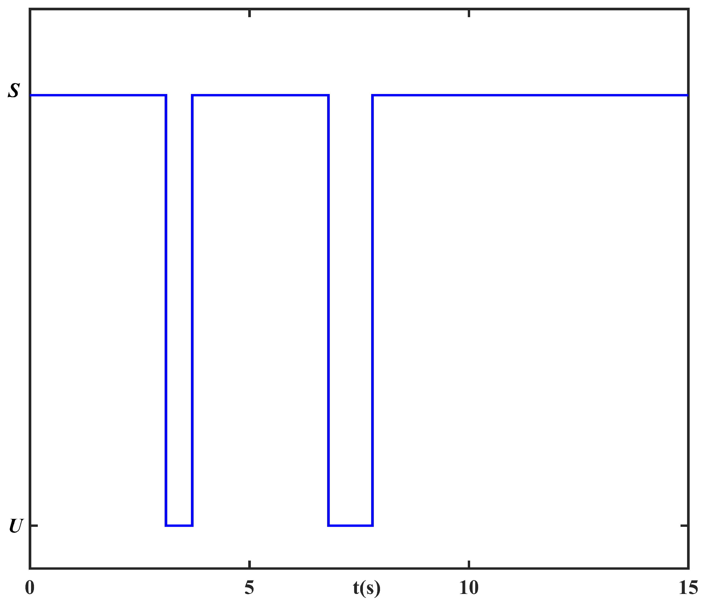
The switched system based on the zero-input method is shown in Figure 1. From Figure 1, it can be observed that the occurrence of packet loss generates a switching signal $\sigma \left(t\right)$, which subsequently determines the value of the feedback controller and activates the corresponding subsystem.

Assumption 2.

In this paper, it is assumed that missing packets only occur in the controller–actuator channel, and δ is employed to represent the loss rate of control packets.

According to the triggering condition in (5), there are $l_k-1$ sampling instants within the triggering interval $(t_{k}h,t_{k+1}h)$. Next, using the partition method, the triggering interval $[t_{k}h,t_{k+1}h)$ can be written as follows:

$$\begin{array}{c}\hfill [t_{k}h,t_{k+1}h)={\bigcup }_{l=0}^{l_k-1}\left[t_{k}h+lh,t_{k}h+(l+1)h\right)={\bigcup }_{l=0}^{l_k-1}{J}_l.\end{array}$$

(10)

We define the time-varying delay ${\theta }_1\left(t\right)=t-(t_{k}h+lh),t\in J_l$, then ${\theta }_1\left(t\right)\in [0,h)$. Thus, one can have the following:

$$\begin{array}{cc}\hfill \tilde{x}\left(t_{k}h\right)& =x(t_{k}h+lh)-\tilde{e}(t_{k}h+lh)=x(t-{\theta }_1\left(t\right))-\tilde{e}(t_{k}h+lh),t\in J_l.\hfill \end{array}$$

(11)

Therefore, the closed-loop system (9) can finally be expressed as follows:

$$\begin{array}{cc}\hfill \dot{x}\left(t\right)=& W_{1}x\left(t\right)+W_{2}f(t,x\left(t\right))+NF\left(t\right)[L_{1}x\left(t\right)+L_{2}f(t,x\left(t\right))]+K_{\sigma \left(t\right)}[x(t-{\theta }_1\left(t\right))-\tilde{e}(t_{k}h+lh)],t\in J_l.\hfill \end{array}$$

(12)

Definition 1

([28]). If there exist $c_1,c_2>0$ satisfying

$${\parallel x\left(t\right)\parallel }^2\le c_1{e}^{-c_2(t-t_0)}·\underset{-\varpi \le s\le 0}{sup}{\parallel x(t_0+s)\parallel }^2,\forall t>t_0.$$

then the closed-loop system (1) is said to be exponentially stable.

Definition 2.

For a switching signal $\sigma \left(t\right)$, if there exists a constant ${\tau }_a>0$, such that

$$N_{\sigma \left(t\right)}(t_1,t_2)\le N_0+{\displaystyle \frac{t_1-t_2}{{\tau }_a}},\forall t_1>t_2\ge 0,$$

holds for $N_0\ge 1$, where $N_{\sigma \left(t\right)}(t_1,t_2)$ stands for the number of switching events on $(t_2,t_1)$, then ${\tau }_a$ is called the average dwell time (ADT) of $\sigma \left(t\right)$.

Lemma 1

([29]). For any continuously differentiable function $x:[a_1,a_2]\to \mathbb{R}$, the following inequality holds for a given matrix $H>0$:

$$\begin{array}{cc}\hfill {\int }_{a_1}^{a_2}{\dot{x}}^T\left(t\right)H\dot{x}\left(t\right)dt\ge & {\displaystyle \frac{1}{a_2-a_1}}{\left(x\left(a_2\right)-x\left(a_1\right)\right)}^{T}H\left(x\left(a_2\right)-x\left(a_1\right)\right)+{\displaystyle \frac{3}{a_2-a_1}}{X}^{T}HX,\hfill \end{array}$$

(13)

where $X=x\left(a_2\right)+x\left(a_1\right)-{\displaystyle \frac{2}{a_2-a_1}}{\int }_{a_1}^{a_2}x\left(t\right)dt$.

3. Main Results

The stability criterion and the controller design for the resulting system (12) will be proposed in this section.

Theorem 1.

For given scalars $\beta >0,\nu >0,\rho >0,{\phi }_1>0,{\phi }_2>0,\varpi >0,{\lambda }_s>0$, ${\lambda }_u<0$, $\mu >1$ and feedback gain matrix K, the closed-loop system in (12) is exponentially stable if there exist matrices $P_s,P_u,Q_s,Q_u,S,\Omega ,\in {\mathbb{R}}_{+}^{n\times n}$, $R=\left[\begin{array}{cc}{R}_{11}& R_{12}\\ \ast & R_{22}\end{array}\right]\in {\mathbb{R}}_{+}^{2n\times 2n}$ and matrices $M_1,M_2\in {\mathbb{R}}^{n\times n}$, such that the following LMIs hold:

$$\begin{array}{cc}\hfill & \left[\begin{array}{cc}{\Sigma }_1& \nu {\Gamma }^T\\ \ast & -\nu I_m\end{array}\right]<0,\hfill \end{array}$$

(14)

$$\begin{array}{cc}\hfill & \left[\begin{array}{cc}{\Sigma }_2& \nu {\Gamma }^T\\ \ast & -\nu I_m\end{array}\right]<0,\hfill \end{array}$$

(15)

$$\begin{array}{cc}\hfill & \left[\begin{array}{cc}\Pi & \nu {\Lambda }^T\\ \ast & -\nu I_m\end{array}\right]<0,\hfill \end{array}$$

(16)

$$\begin{array}{cc}\hfill & P_u\le \mu P_s,Q_u\le \mu e^{-({\lambda }_s-{\lambda }_u)·\varpi }{Q}_s,\hfill \end{array}$$

(17)

$$\begin{array}{cc}\hfill & P_s\le \mu P_u,Q_s\le \mu Q_u,\hfill \end{array}$$

(18)

where ${\Sigma }_1,{\Sigma }_2\in {\mathbb{R}}^{(7n+m)\times (7n+m)}$ and $\Pi \in {\mathbb{R}}^{(3n+m)\times (3n+m)}$ are symmetric matrices, and ${\Sigma }_1(1,1)={\lambda }_s{P}_s-\frac{4e^{-{\lambda }_{s}h}}{h}{R}_{11}+{\phi }_1{M}_1{W}_1+{\phi }_1{W}_1^T{M}_1^T+Q_s+{\beta }^2{H}^{T}H+(\frac{{\lambda }_s}{4}{h}^2-h)S$, ${\Sigma }_1(1,2)=$${\Sigma }_2(1,2)=P_s-{\phi }_1{M}_1+{\phi }_2{W}_1^T{M}_2^T+\frac{h^2}{4}S$, ${\Sigma }_1(1,3)={\Sigma }_2(1,3)={\phi }_1{M}_1{W}_2$, ${\Sigma }_1(1,4)={\Sigma }_2(1,4)={\phi }_1{M}_{1}N$, ${\Sigma }_1(1,5)={\Sigma }_2(1,5)=\frac{-2e^{-{\lambda }_{s}h}}{h}{R}_{11}-e^{-{\lambda }_{s}h}{R}_{12}+{\phi }_1{M}_{1}K$, ${\Sigma }_1(1,6)={\Sigma }_2(1,6)=-{\phi }_1{M}_{1}K$, ${\Sigma }_1(1,7)={\Sigma }_2(1,7)=\frac{6e^{-{\lambda }_{s}h}}{h}{R}_{11}$, ${\Sigma }_1(2,2)=-{\phi }_2(M_2+M_2^T)$, ${\Sigma }_1(2,3)={\Sigma }_2(2,3)={\phi }_2{M}_2{W}_2$, ${\Sigma }_1(2,4)={\Sigma }_2(2,4)={\phi }_2{M}_{2}N$, ${\Sigma }_1(2,5)={\phi }_2{M}_{2}K$, ${\Sigma }_1(2,6)={\Sigma }_2(2,6)=-{\phi }_2{M}_{2}K$, ${\Sigma }_1(3,3)={\Sigma }_2(3,3)=-I_m$, ${\Sigma }_1(4,4)={\Sigma }_2(4,4)=-\nu I_m$, ${\Sigma }_1(5,5)={\Sigma }_2(5,5)=\frac{-4e^{-{\lambda }_{s}h}}{h}{R}_{11}+2e^{-{\lambda }_{s}h}{R}_{12}+\rho \Omega -h{e}^{-{\lambda }_{s}h}{R}_{22}$, ${\Sigma }_1(5,6)={\Sigma }_2(5,6)=-\rho \Omega$, ${\Sigma }_1(5,7)={\Sigma }_2(5,7)=\frac{6e^{-{\lambda }_{s}h}}{h}{R}_{11}$, ${\Sigma }_1(6,6)={\Sigma }_2(6,6)=(\rho -1)\Omega$, ${\Sigma }_1(7,7)={\Sigma }_2(7,7)=\frac{-12e^{-{\lambda }_{s}h}}{h}{R}_{11}$, ${\Sigma }_1(8,8)={\Sigma }_2(8,8)=-e^{-{\lambda }_s\varpi }{Q}_s$, ${\Sigma }_2(1,1)={\lambda }_s{P}_s-\frac{4e^{-{\lambda }_{s}h}}{h}{R}_{11}+{\phi }_1{M}_1{W}_1+{\phi }_1{W}_1^T{M}_1^T+Q_s+{\beta }^2{H}^{T}H+(\frac{{\lambda }_s}{4}{h}^2+h)S$, ${\Sigma }_2(2,2)=-{\phi }_2(M_2+M_2^T)+h{R}_{11}$, ${\Sigma }_2(2,5)={\phi }_2{M}_{2}K+h{R}_{12}$, ${\Sigma }_2(5,5)=\frac{-4e^{-{\lambda }_{s}h}}{h}{R}_{11}+2e^{-{\lambda }_{s}h}{R}_{12}+\rho \Omega +h{R}_{22}$, $\Pi (1,1)=P_u{W}_1+W_1^T{P}_u^T+{\lambda }_u{P}_u+{\beta }^2{H}^{T}H+Q_u$, $\Pi (1,2)=P_u{W}_2$, $\Pi (1,3)=P_{u}N$, $\Pi (2,2)=-I_m$, $\Pi (3,3)=-\nu I_m$, $\Pi (4,4)=-Q_u$, $\Gamma =\left[L_1{0}_{m\times n}{L}_2{0}_{m\times m}{0}_{m\times n}{0}_{m\times n}{0}_{m\times n}{0}_{m\times n}\right]$, $\Lambda =\left[L_1{L}_2{0}_{m\times m}{0}_{m\times n}\right]$. The ADT ${\tau }_a$ and the pocket loss rate δ satisfy the following constraints:

$${\tau }_a>{\displaystyle \frac{ln\mu }{{\lambda }_s(1-\delta )+{\lambda }_u\delta }},\delta <{\displaystyle \frac{{\lambda }_s}{{\lambda }_s-{\lambda }_u}}.$$

(19)

Proof. 

Consider a Lyapunov functional $V\left(t\right)$ as follows, where $V_s\left(t\right)$ is for the stable subsystem (7) and $V_u\left(t\right)$ is for the unstable subsystem (8):

$$V\left(t\right)=V_{\sigma \left(t\right)}\left(t\right)=\left\{\begin{array}{c}{V}_s\left(t\right),\mathrm{for}\sigma \left(t\right)=s\hfill \\ V_u\left(t\right),\mathrm{for}\sigma \left(t\right)=u\hfill \end{array}\right.,t\in J_l,$$

with

$$\begin{array}{cc}\hfill V_s\left(t\right)=& {\sum }_{i=1}^4{V}_{si}\left(t\right),\hfill \\ \hfill =& x{\left(t\right)}^T{P}_{s}x\left(t\right)+\frac{1}{\varpi }{\int }_{-\varpi }^0{\int }_{t+v}^t{e}^{{\lambda }_s(s-t)}x{\left(s\right)}^T{Q}_{s}x\left(s\right)dsdv\hfill \\ \hfill & +{\theta }_2\left(t\right){\int }_{t-{\theta }_1\left(t\right)}^t{e}^{{\lambda }_s(s-t)}{\left[\begin{array}{c}\dot{x}\left(s\right)\\ x(t-{\theta }_1\left(t\right))\end{array}\right]}^{T}R\left[\begin{array}{c}\dot{x}\left(s\right)\\ x(t-{\theta }_1\left(t\right))\end{array}\right]ds+{\theta }_1\left(t\right){\theta }_2\left(t\right)x{\left(t\right)}^{T}Sx\left(t\right),\hfill \end{array}$$

(20)

$$\begin{array}{cc}\hfill V_u\left(t\right)=& {\sum }_{i=1}^2{V}_{ui}\left(t\right),\hfill \\ \hfill =& x{\left(t\right)}^T{P}_{u}x\left(t\right)+\frac{1}{\varpi }{\int }_{-\varpi }^0{\int }_{t+v}^t{e}^{{\lambda }_u(s-t)}x{\left(s\right)}^T{Q}_{u}x\left(s\right)dsdv,\hfill \end{array}$$

(21)

in which ${\theta }_1\left(t\right)=t-(t_{k}h+lh)$, ${\theta }_2\left(t\right)=t_{k}h+(l+1)h-t$, and ${\lambda }_s>0$, ${\lambda }_u<0$ are given constants.

Case 1: When the closed-loop system (12) is in the stable subsystem, the derivative of $V_s\left(t\right)$ along the trajectory of the stable subsystem (7) is as follows:

$$\begin{array}{cc}\hfill & \dot{V_s}\left(t\right)+{\lambda }_s{V}_s\left(t\right)\hfill \\ \hfill \le & 2x{\left(t\right)}^T{P}_s\dot{x}\left(t\right)+{\lambda }_{s}x{\left(t\right)}^T{P}_{s}x\left(t\right)+x{\left(t\right)}^T{Q}_{s}x\left(t\right)-\frac{1}{\varpi }{\int }_{-\varpi }^0{e}^{{\lambda }_{s}v}x{(t+v)}^T{Q}_{s}x(t+v)dv\hfill \\ \hfill & -{\int }_{t-{\theta }_1\left(t\right)}^t{e}^{-{\lambda }_{s}h}{\dot{x}}^T\left(s\right)R_{11}\dot{x}\left(s\right)ds-2e^{-{\lambda }_{s}h}{\left[x\left(t\right)-x(t-{\theta }_1\left(t\right))\right]}^T{R}_{12}x(t-{\theta }_1\left(t\right))\hfill \\ \hfill & -{\theta }_1\left(t\right)e^{-{\lambda }_{s}h}{x}^T(t-{\theta }_1\left(t\right))R_{22}x(t-{\theta }_1\left(t\right))+{\theta }_2\left(t\right){\left[\begin{array}{c}\dot{x}\left(t\right)\\ x(t-{\theta }_1\left(t\right))\end{array}\right]}^{T}R\left[\begin{array}{c}\dot{x}\left(t\right)\\ x(t-{\theta }_1\left(t\right))\end{array}\right]\hfill \\ \hfill & +[{\theta }_2\left(t\right)-{\theta }_1\left(t\right)]x{\left(t\right)}^{T}Sx\left(t\right)+2{\theta }_1\left(t\right){\theta }_2\left(t\right)x{\left(t\right)}^{T}S\dot{x}\left(t\right)+{\lambda }_s{\theta }_1\left(t\right){\theta }_2\left(t\right)x{\left(t\right)}^{T}Sx\left(t\right).\hfill \end{array}$$

(22)

By applying Jensen’s inequality to the first integral term in (22), one obtains the following:

$$\begin{array}{cc}\hfill -\frac{1}{\varpi }{\int }_{-\varpi }^0{e}^{{\lambda }_{s}v}x{(t+v)}^T{Q}_{s}x(t+v)dv& =-\frac{1}{\varpi }{\int }_{t-\varpi }^t{e}^{{\lambda }_s(s-t)}{x}^T\left(s\right)Q_{s}x\left(s\right)ds,\hfill \\ \hfill & \le -\frac{1}{\varpi }{\int }_{t-\varpi }^t{e}^{-{\lambda }_s\varpi }{x}^T\left(s\right)Q_{s}x\left(s\right)ds,\hfill \\ \hfill & \le -e^{-{\lambda }_s\varpi }{\left[\frac{1}{\varpi }{\int }_{t-\varpi }^{t}x\left(s\right)ds\right]}^T{Q}_s\left[\frac{1}{\varpi }{\int }_{t-\varpi }^{t}x\left(s\right)ds\right],\hfill \\ \hfill & =-e^{-{\lambda }_s\varpi }{\tilde{x}}^T\left(t\right)Q_s\tilde{x}\left(t\right),\hfill \end{array}$$

(23)

with $\tilde{x}\left(t\right)=\frac{1}{\varpi }{\int }_{t-\varpi }^{t}x\left(s\right)ds$.

In terms of Lemma 1, the second integral term in (22) can be estimated as follows:

$$\begin{array}{c}\hfill -{\int }_{t-{\theta }_1\left(t\right)}^t{e}^{-{\lambda }_{s}h}{\dot{x}}^T\left(s\right)R_{11}\dot{x}\left(s\right)ds<-{\displaystyle \frac{e^{-{\lambda }_{s}h}}{h}}{\left[\begin{array}{c}x\left(t\right)\\ x(t-{\theta }_1\left(t\right))\\ \epsilon \left(t\right)\end{array}\right]}^T\left[\begin{array}{ccc}4R_{11}& 2R_{11}& -6R_{11}\\ \ast & 4R_{11}& -6R_{11}\\ \ast & \ast & 12R_{11}\end{array}\right]\left[\begin{array}{c}x\left(t\right)\\ x(t-{\theta }_1\left(t\right))\\ \epsilon \left(t\right)\end{array}\right],\end{array}$$

(24)

where $\epsilon \left(t\right)=\frac{1}{{\theta }_1\left(t\right)}{\int }_{t-{\theta }_1\left(t\right)}^{t}x\left(s\right)ds$.

Utilizing the free-weighing matrix method, the following equation holds for constants ${\phi }_1>0$, ${\phi }_2>0$ and appropriate dimension matrices $M_1,M_2$:

$$\begin{array}{cc}\hfill & \left[2{\phi }_1{x}^T\left(t\right)M_1+2{\phi }_2{\dot{x}}^T\left(t\right)M_2\right]\hfill \\ \hfill & \times \left[-\dot{x}\left(t\right)+W_{1}x\left(t\right)+W_{2}f(t,x\left(t\right))+Nq\left(t\right)+K\left(x(t-{\theta }_1\left(t\right))-\tilde{e}(t_{k}h+lh)\right)\right]=0,\hfill \end{array}$$

(25)

in which $q\left(t\right)=F\left(t\right)p\left(t\right)$ and $p\left(t\right)=L_{1}x+L_{2}f(t,x\left(t\right))$.

Meanwhile, based on (4), one obtains $q^T\left(t\right)q\left(t\right)\le p^T\left(t\right)p\left(t\right)$; then, for constant $\nu >0$, it follows that

$$\nu \left[{\varsigma }^T\left(t\right){\Gamma }^T\Gamma \varsigma \left(t\right)-q^T\left(t\right)q\left(t\right)\right]\ge 0,$$

(26)

where $\varsigma \left(t\right)=\mathrm{col}\{x\left(t\right),\dot{x}\left(t\right),f(t,x\left(t\right)),q\left(t\right),x(t-{\theta }_1\left(t\right)),\tilde{e}(t_{k}h+lh),\epsilon \left(t\right),\tilde{x}\left(t\right)\}$, $\Gamma =[L_1{0}_{m\times n}$$L_2{0}_{m\times m}{0}_{m\times n}{0}_{m\times n}{0}_{m\times n}{0}_{m\times n}]$.

Substituting (2), (5), (23)–(26) into (22), and considering the fact that

$${\theta }_1\left(t\right){\theta }_2\left(t\right)\le {\displaystyle \frac{{({\theta }_1\left(t\right)+{\theta }_2\left(t\right))}^2}{4}}={\displaystyle \frac{h({\theta }_1\left(t\right)+{\theta }_2\left(t\right))}{4}},$$

we can have

$$\begin{array}{c}\hfill \dot{V_s}\left(t\right)+{\lambda }_s{V}_s\left(t\right)\le {\varsigma }^T\left(t\right)\left\{{\displaystyle \frac{{\theta }_1\left(t\right)}{h}}({\Sigma }_1+\nu {\Gamma }^T\Gamma )+{\displaystyle \frac{{\theta }_2\left(t\right)}{h}}({\Sigma }_2+\nu {\Gamma }^T\Gamma )\right\}\varsigma \left(t\right),\end{array}$$

where ${\Sigma }_1,{\Sigma }_2$ are defined in Theorem 1. Next, according to LMIs (14) and (15), one can finally obtain the following:

$$\dot{V_s}\left(t\right)+{\lambda }_s{V}_s\left(t\right)<0.$$

(27)

Case 2: When the closed-loop system (12) is in the unstable subsystem, taking the derivation of $V_u\left(t\right)$ yields the following:

$$\begin{array}{cc}\hfill & \dot{V_u}\left(t\right)+{\lambda }_u{V}_u\left(t\right)\hfill \\ \hfill =& 2x{\left(t\right)}^T{P}_u\dot{x}\left(t\right)+{\lambda }_{s}x{\left(t\right)}^T{P}_{u}x\left(t\right)+x{\left(t\right)}^T{Q}_{u}x\left(t\right)-\frac{1}{\varpi }{\int }_{-\varpi }^0{e}^{{\lambda }_{u}v}x{(t+v)}^T{Q}_{u}x(t+v)dv.\hfill \end{array}$$

(28)

With the same operation, we give the estimation of the integral term in (28) as follows:

$$\begin{array}{c}\hfill -\frac{1}{\varpi }{\int }_{-\varpi }^0{e}^{{\lambda }_{u}v}x{(t+v)}^T{Q}_{u}x(t+v)dv\le -{\tilde{x}}^T\left(t\right)Q_u\tilde{x}\left(t\right),\end{array}$$

(29)

in which $\tilde{x}\left(t\right)=\frac{1}{\varpi }{\int }_{t-\varpi }^{t}x\left(s\right)ds$.

Simultaneously, we have the following identical equation and inequality:

$$\nu \left[{\eta }^T\left(t\right){\Lambda }^T\Lambda \eta \left(t\right)-q^T\left(t\right)q\left(t\right)\right]\ge 0,$$

(30)

where $\eta \left(t\right)=\mathrm{col}\{x\left(t\right),f(t,x\left(t\right)),q\left(t\right),\tilde{x}\left(t\right)\}$ and $\Lambda =\left[L_1{L}_2{0}_{m\times m}{0}_{m\times n}\right]$.

Combining with (2), (28)–(30), one has the following:

$$\begin{array}{c}\hfill \dot{V_u}\left(t\right)+{\lambda }_u{V}_u\left(t\right)\le {\eta }^T\left(t\right)\left(\Pi +\nu {\Lambda }^T\Lambda \right)\eta \left(t\right).\end{array}$$

(31)

Based on (16), one can conclude the following:

$$\dot{V_u}\left(t\right)+{\lambda }_u{V}_u\left(t\right)<0.$$

(32)

Furthermore, synthesizing (27) and (32), one can now obtain that

$$\dot{V}\left(t\right)+\lambda V\left(t\right)<0,$$

(33)

in which $\lambda ={\lambda }_{\sigma \left(t\right)}=\left\{\begin{array}{cc}{\lambda }_s,\hfill & \mathrm{for}\sigma \left(t\right)=s,\hfill \\ {\lambda }_u,\hfill & \mathrm{for}\sigma \left(t\right)=u.\hfill \end{array}\right.$

Moreover, we denote $\left\{{\tau }_l\right\}$ as the switching series between the stable subsystem and the unstable subsystem during $(0,t)$. Then, the triggering instant ${\tau }_l$ may be transmitted or lost. In what follows, these two cases will be discussed in detail.

If ${\tau }_l$ is the lost triggering instant, then one has the following:

$$\begin{array}{cc}\hfill & V\left({\tau }_l^{-}\right)=V_s\left({\tau }_l^{-}\right)=V_{s1}\left({\tau }_l\right)+V_{s2}\left({\tau }_l\right),\hfill \\ \hfill & V\left({\tau }_l\right)=V_u\left({\tau }_l\right)=V_{u1}\left({\tau }_l\right)+V_{u2}\left({\tau }_l\right).\hfill \end{array}$$

In terms of the condition in (17), one further has

$$V\left({\tau }_l\right)\le \mu V\left({\tau }_l^{-}\right).$$

(34)

If ${\tau }_l$ is the transmitted triggering instant, then based on (18), the same result $V\left({\tau }_l\right)\le \mu V\left({\tau }_l^{-}\right)$ can still be obtained.

During the interval $(0,t)$, we denote $T_s(0,t)$ and $T_u(0,t)$ as the total length of all stable intervals and the total length of all unstable intervals, respectively. Obviously, the loss rate of control packet $\delta$ can be represented as follows:

$$\delta ={\displaystyle \frac{T_u\left(t\right)}{t}}.$$

(35)

Let ${\tau }_q$ be the switching instant nearest to t. Due to the condition (27), (32), and (34)–(35), the following holds:

$$\begin{array}{cc}\hfill V\left(t\right)& \le e^{-{\lambda }_{\sigma \left({\tau }_q\right)}(t-{\tau }_q)}{V}_{\sigma \left({\tau }_q\right)}\left({\tau }_q\right),\hfill \\ \hfill & \le \mu e^{-{\lambda }_{\sigma \left({\tau }_q\right)}(t-{\tau }_q)}{V}_{\sigma \left({\tau }_q^{-}\right)}\left({\tau }_q^{-}\right),\hfill \\ \hfill & ⋮\hfill \\ \hfill & \le {\mu }^{N_{\sigma \left(t\right)}(t,0)}{e}^{-{\lambda }_s{T}_s(0,t)}{e}^{-{\lambda }_u{T}_u(0,t)}V\left(0\right),\hfill \\ \hfill & \le {\mu }^{N_0+\frac{t}{{\tau }_a}}{e}^{-{\lambda }_s(t-\delta t)-{\lambda }_u\delta t}V\left(0\right),\hfill \\ \hfill & ={ϵ}_1{e}^{-{ϵ}_{2}t}V\left(0\right),\hfill \end{array}$$

(36)

with ${ϵ}_1=e^{N_{0}ln\mu }$, ${ϵ}_2={\lambda }_s(1-\delta )+{\lambda }_u\delta -\frac{ln\mu }{{\tau }_a}$.

In line with (20) and (21), one can obtain

$$V\left(t\right)\ge {\lambda }_1{\parallel x\left(t\right)\parallel }^2,$$

and

$$\begin{array}{cc}\hfill V\left(0\right)& \le {\lambda }_2{\parallel x\left(0\right)\parallel }^2+\varpi ·{\lambda }_3\underset{-\varpi \le s\le 0}{sup}{\parallel x\left(s\right)\parallel }^2\le {ϵ}_3\underset{-\varpi \le s\le 0}{sup}{\parallel x\left(s\right)\parallel }^2,\hfill \end{array}$$

in which ${\lambda }_1=min\{{\lambda }_{min}\left\{P_s\right\},{\lambda }_{min}\left\{P_u\right\}\}$, ${\lambda }_2=max\{{\lambda }_{max}\left\{P_s\right\},{\lambda }_{max}\left\{P_u\right\}\}$, ${\lambda }_3=max\{{\lambda }_{max}\left\{Q_s\right\},{\lambda }_{max}\left\{Q_u\right\}\}$ and ${ϵ}_3={\lambda }_2+\varpi ·{\lambda }_3$.

Considering (36), the following inequality can be deduced:

$$\begin{array}{cc}\hfill & {\parallel x\left(t\right)\parallel }^2\le {ϵ}_4{e}^{-{ϵ}_{2}t}\underset{-\varpi \le s\le 0}{sup}{\parallel x\left(s\right)\parallel }^2,\hfill \end{array}$$

where ${ϵ}_4=\frac{{ϵ}_1{ϵ}_3}{{\lambda }_1}$. Thus, based on Definition 1, the system (12) is exponentially stable. □

Remark 3.

Looped functionals $V_{s3}\left(t\right)$ and $V_{s4}\left(t\right)$ can result in $V_{s3}(t_{k}h+lh)=V_{s3}(t_{k}h+(l+1)h)=0$ and $V_{s4}(t_{k}h+lh)=V_{s4}(t_{k}h+(l+1)h)=0$, in which $t_{k}h+lh$ and $t_{k}h+(l+1)h$ are sampling instants. Given that the switching instant ${\tau }_l$ comes from the set of sampling instants, it follows that $V_{s3}\left({\tau }_l\right)=0$ and $V_{s4}\left({\tau }_l\right)=0$. As a result, $V_{s3}\left(t\right)$ and $V_{s4}\left(t\right)$ will not appear during the analysis of $V\left({\tau }_l\right)\le \mu V\left({\tau }_l^{-}\right)$. This enables LMIs for system stability to be simplified, consequently enlarging the feasible region of the LMIs. Additionally, looped functionals $V_{s3}\left(t\right)$ and $V_{s4}\left(t\right)$ can fully utilize the system information over $[x(t_{k}h+lh),x\left(t\right))$ and $[x\left(t\right),x(t_{k}h+(l+1)h))$, which contributes to obtaining results with reduced conservatism.

Next, the controller design for the system (1) based on the aforementioned analysis will be given by employing the matrix decoupling method.

Theorem 2.

For given positive scalars β, ν, ρ, ϖ, ${\lambda }_s$, κ, ${\phi }_1$, ${\phi }_2$, $\mu >1$ and negative scalar ${\lambda }_u$, the closed-loop system (1) is exponentially stable under the design of control gain matrix $K=M_1^{-1}\widehat{K}$ if there exist matrices $P_s,P_u,Q_s,Q_u,S,\Omega \in {\mathbb{R}}_{+}^{n\times n}$, $R\in {\mathbb{R}}_{+}^{2n\times 2n}$, arbitrary matrices $M_1,\widehat{K}$, such that the following LMIs hold:

$$\begin{array}{cc}\hfill & \left[\begin{array}{cc}{\widehat{\Sigma }}_1& \nu {\Gamma }^T\\ \ast & -\nu I_m\end{array}\right]<0,\hfill \end{array}$$

(37)

$$\begin{array}{cc}\hfill & \left[\begin{array}{cc}{\widehat{\Sigma }}_2& \nu {\Gamma }^T\\ \ast & -\nu I_m\end{array}\right]<0,\hfill \end{array}$$

(38)

$$\begin{array}{cc}\hfill & \left[\begin{array}{cc}\Pi & \nu {\Lambda }^T\\ \ast & -\nu I_m\end{array}\right]<0,\hfill \end{array}$$

(39)

$$\begin{array}{cc}\hfill & P_u\le \mu P_s,Q_u\le \mu e^{-({\lambda }_s-{\lambda }_u)·\varpi }{Q}_s,\hfill \end{array}$$

(40)

$$\begin{array}{cc}\hfill & P_s\le \mu P_u,Q_s\le \mu Q_u,\hfill \end{array}$$

(41)

where ${\widehat{\Sigma }}_1,{\widehat{\Sigma }}_2\in {\mathbb{R}}^{(7n+m)\times (7n+m)}$ and $\Pi \in {\mathbb{R}}^{(3n+m)\times (3n+m)}$ are symmetric matrices, and ${\widehat{\Sigma }}_1(1,2)={\widehat{\Sigma }}_2(1,2)=P_s-{\phi }_1{M}_1+\kappa {\phi }_2{W}_1^T{M}_1^T+\frac{h^2}{4}S$, ${\widehat{\Sigma }}_1(1,5)={\widehat{\Sigma }}_2(1,5)=\frac{-2e^{-{\lambda }_{s}h}}{h}{R}_{11}-e^{-{\lambda }_{s}h}{R}_{12}+{\phi }_1\widehat{K}$, ${\widehat{\Sigma }}_1(1,6)={\widehat{\Sigma }}_2(1,6)=-{\phi }_1\widehat{K}$, ${\widehat{\Sigma }}_1(2,2)=-\kappa {\phi }_2(M_1+M_1^T)$, ${\widehat{\Sigma }}_2(2,2)=-\kappa {\phi }_2(M_1+M_1^T)+h{R}_{11}$, ${\widehat{\Sigma }}_1(2,3)={\widehat{\Sigma }}_2(2,3)=\kappa {\phi }_2{M}_1{W}_2$, ${\widehat{\Sigma }}_1(2,4)={\widehat{\Sigma }}_2(2,4)=\kappa {\phi }_2{M}_{1}N$, ${\widehat{\Sigma }}_1(2,5)=\kappa {\phi }_2\widehat{K}$, ${\widehat{\Sigma }}_2(2,5)=\kappa {\phi }_2\widehat{K}+h{R}_{12}$, ${\widehat{\Sigma }}_1(2,6)={\widehat{\Sigma }}_2(2,6)=-\kappa {\phi }_2\widehat{K}$, the other blocks of ${\widehat{\Sigma }}_1$, ${\widehat{\Sigma }}_2$ have the same definition as those of ${\Sigma }_1,{\Sigma }_2$ in Theorem 1, and the ADT and the pocket loss rate satisfy ${\tau }_a>{\displaystyle \frac{ln\mu }{{\lambda }_s(1-\delta )+{\lambda }_u\delta }}$ and $\delta <{\displaystyle \frac{{\lambda }_s}{{\lambda }_s-{\lambda }_u}}$.

Proof. 

We define $M_2=\kappa M_1,\widehat{K}=M_{1}K$. Then, LMIs (14)–(18) can be represented as (37)–(41). Based on (37)–(41), one can calculate the gain matrix $K=M_1^{-1}\widehat{K}$, which achieve the proof. □

4. Numerical Simulation

In this section, a numerical example will be employed to demonstrate the effectiveness of the proposed IMET scheme.

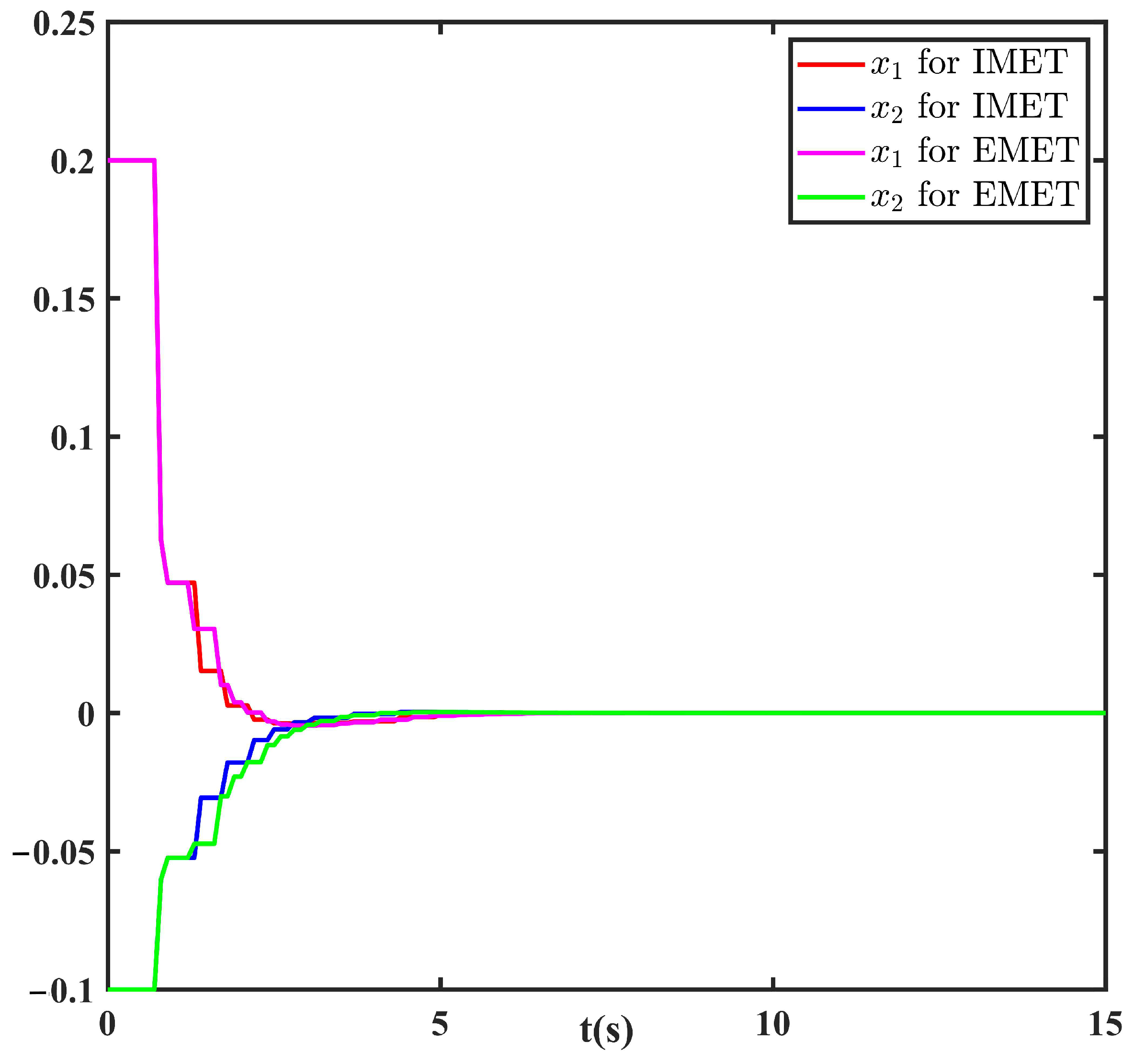
Example 1.

Consider the following NN with the following uncertainties:

$$\begin{array}{cc}\hfill & W_1=\left[\begin{array}{cc}-1.8& 0\\ 0& -1.9\end{array}\right],W_2=\left[\begin{array}{cc}2.79& 1\\ -1& 2.5\end{array}\right],N=\left[\begin{array}{c}0.02\\ 0.01\end{array}\right],f(t,x\left(t\right))=\left[\begin{array}{c}0.5sin\left(x_1\left(t\right)\right)\\ 0.5sin\left(x_2\left(t\right)\right)\end{array}\right],\hfill \\ \hfill & L_1=\left[\begin{array}{cc}-0.01& 0.01\end{array}\right],L_2=\left[\begin{array}{cc}-0.02& -0.01\end{array}\right],F\left(t\right)=0.6+0.3\sin t.\hfill \end{array}$$

The initial condition is chosen as $x\left(0\right)={(0.2,-0.1)}^T$. We select ${\lambda }_s=0.2,{\lambda }_u=-0.1$, then the loss rate is calculated as $\delta <0.667$ based on Condition (19) in Theorem 1. Then, we set $\delta =0.1$ and $\mu =1.1$, and the ADT is calculated as ${\tau }_a>0.561$. We take $\kappa =1.1,\rho =0.3,\varpi =0.2,\beta =0.6$ and constant matrix $H=I_2$; then, the control gain matrix and the triggering parameter Ω are calculated based on Theorem 2 as follows:

$$\begin{array}{c}\hfill K=\left[\begin{array}{cc}-0.418& 0.141\\ 0.098& -0.498\end{array}\right],\Omega =\left[\begin{array}{cc}5.667& -2.746\\ -2.746& 8.824\end{array}\right].\end{array}$$

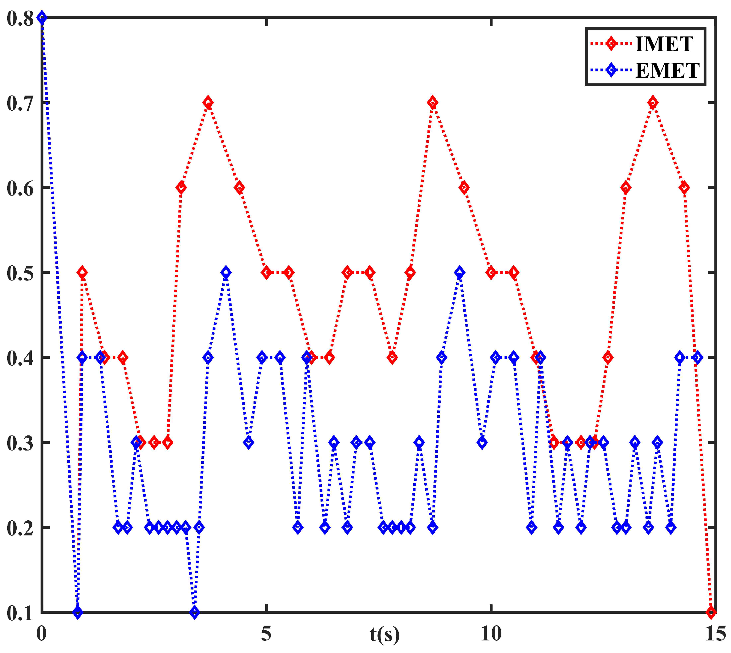
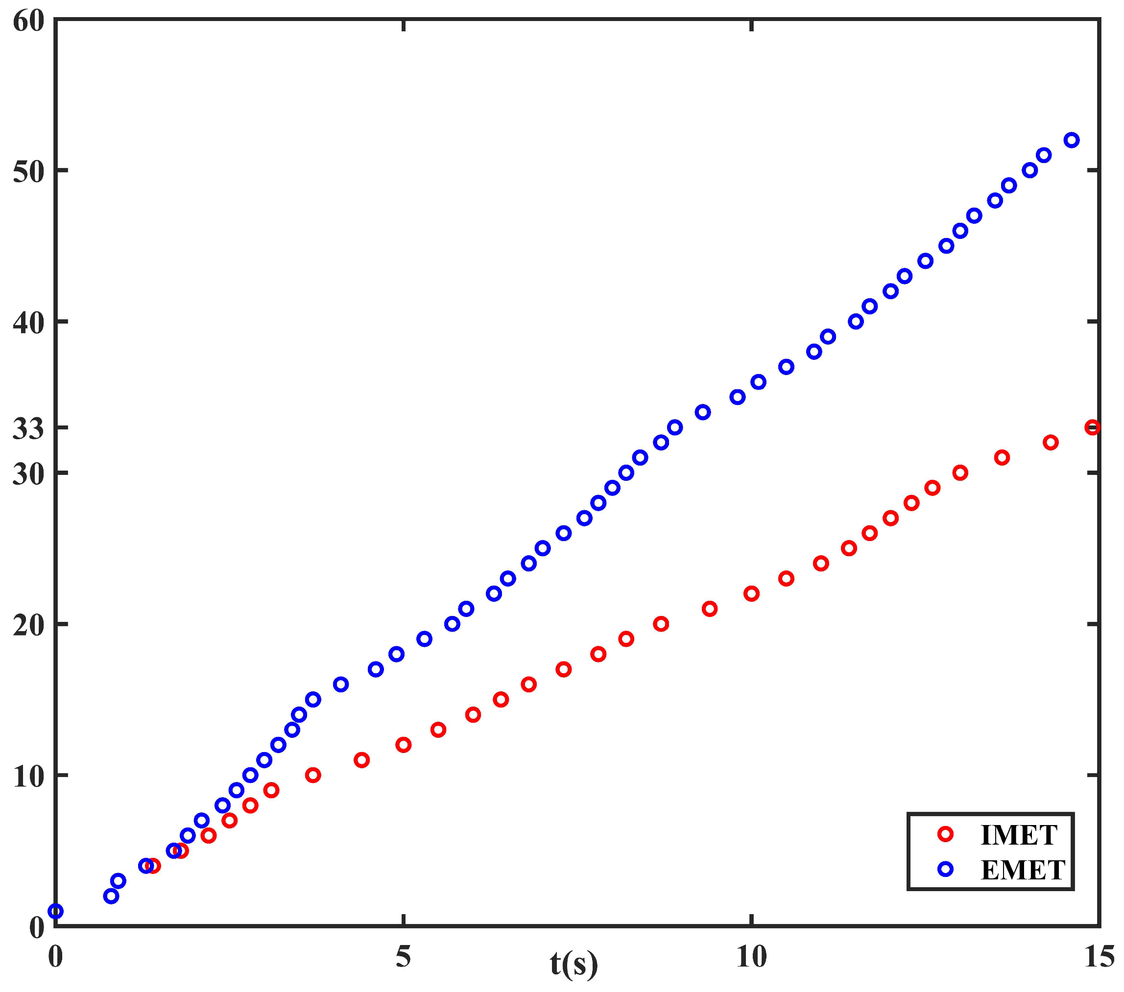
The state responses under the EMET and the IMET are shown in Figure 2. It is clear that the system trajectories obtained via the IMET scheme are gentler and can converge to zero much faster than the ones obtained by the EMET. This means that the IMET can ensure better system performance. Figure 3 and Figure 4 present the execution interval and the cumulative triggering times for the EMET scheme and the IMET scheme, respectively. One can determine that the triggering interval of the IMET is larger that of the EMET. Meanwhile, the total triggering number for the IMET scheme is 33, which is less than 52 obtained via the EMET scheme. Combining Figure 2, Figure 3 and Figure 4, one can conclude that the proposed IMET scheme can reduce the network burden on the premise of ensuring good system performance.

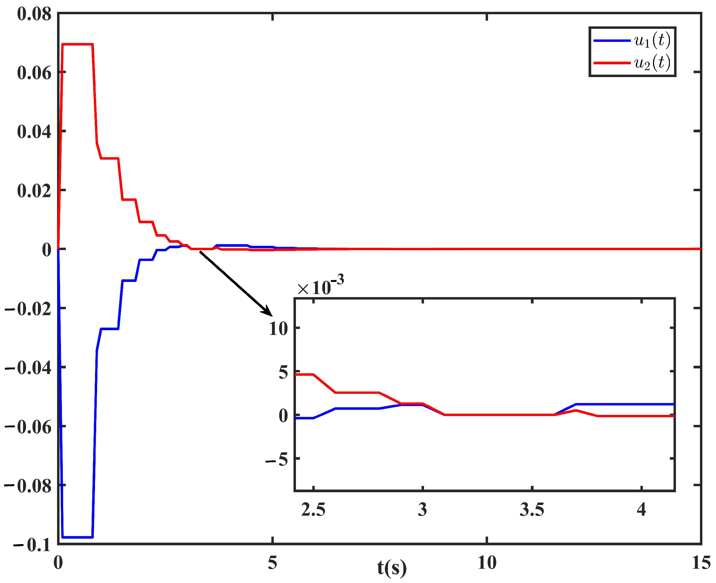
Figure 5 displays the trajectories of the control input under the IMET scheme with packet loss rate $\delta =0.1$. The intervals corresponding to $u=0$ suggest that the system is under the unstable subsystem. The starting points of these intervals are the moments when the packets are lost, and the end points are the moments when the system is under the controller again. Meanwhile, the switching signal $\sigma \left(t\right)$ is shown in Figure 6.

5. Conclusions

In this paper, by employing the zero-input method, the stabilization problem of an uncertain NN with missing input is converted into the stability problem of a switched system and then is addressed by developing an IMET scheme. Compared with the EMET scheme, the proposed IMET scheme is based on the PET scheme and therefore can prevent Zeno behavior naturally. Moreover, it introduces an integral over a past time interval of the latest triggering instant to construct the triggering condition. Therefore, even if the packets close to the current trigger are missing, it can still employ the integral to cover the information of the system with packet loss. To study the switched closed-loop system, a new piecewise Lyapunov functional is designed, which not only contains a looped functional to fully use the state information but also contains a Lyapunov functional involving the memory period of the IMET scheme. Then, by using this functional and combining with some inequalities, we establish sufficient conditions that guarantee the exponential stability of the resulting closed-loop system. Finally, an example is provided to analyze the validity of the obtained results.

References

1. Karthick, S.A.; Chen, B.S. Hybrid-triggered and fault-tolerant observer-based control for neural networks under malicious attacks. Neurocomputing 2023, 532, 114–128. [Google Scholar] [CrossRef]
2. Feng, H.K.; Wu, Z.Y.; Zhang, X.X.; Xiao, Z.H.; Zhang, M.; Tao, J. Secure adaptive event-triggered anti-synchronization for BAM neural networks with energy-limited DoS attacks. Inf. Sci. 2024, 670, 120594. [Google Scholar] [CrossRef]
3. Cheng, J.; Xu, J.M.; Yan, H.C.; Wu, Z.H.; Qi, W.H. Neural network-based sliding mode control for semi-markov jumping systems with singular perturbation. IEEE Trans. Cybern. 2025, 55, 259–268. [Google Scholar] [CrossRef]
4. Vadivel, R.; Hammachukiattikul, P.; Gunasekaran, N.; Saravanakumarc, R.; Duttad, H. Strict dissipativity synchronization for delayed static neural networks: An event-triggered scheme. Chaos Solitons Fractals 2021, 150, 111212. [Google Scholar] [CrossRef]
5. Wang, Z.H.; Zhang, L.S.; Raissi, T.; Shen, Y. Interval estimation for discrete-time takagi-sugeno fuzzy nonlinear systems with parameter uncertainties. IEEE Trans. Fuzzy Syst. 2024, 32, 2639–2649. [Google Scholar] [CrossRef]
6. Li, C.S.; Guo, H.; Fu, J.; Pang, H.B. H∞ control for switched non-linear systems with structural uncertainty by using robust passivity. Nonlinear Anal. Hybrid Syst. 2021, 40, 101017. [Google Scholar]
7. Fan, H.G.; Chen, X.J.; Shi, K.B.; Liang, Y.H.; Wang, Y.; Wen, H. Mittag-leffler synchronization in finite time for uncertain fractional-order multi-delayed memristive neural networks with time-varying perturbations via information feedback. Fractal Fract. 2024, 8, 422. [Google Scholar] [CrossRef]
8. Zhang, W.A.; Yu, L. Stabilization of sampled-data control systems with control inputs missing. IEEE Trans. Autom. Control 2010, 55, 447–452. [Google Scholar] [CrossRef]
9. Hu, Z.P.; Chen, K.; Deng, F.Q.; Luo, S.X.; Hu, S.L. H controller design for networked systems with two-channel packet dropouts and FDI attacks. IEEE Trans. Cybern. 2024, 54, 1661–1670. [Google Scholar] [CrossRef] [PubMed]
10. Zhao, F.L.; Wang, Z.P.; Wu, H.N.; Wang, J.L.; Huang, T.W. Output synchronization of reaction-diffusion neural networks under random packet losses via event-triggered sampled-data control. Neurocomputing 2022, 514, 563–573. [Google Scholar] [CrossRef]
11. Lu, R.Q.; Shi, P.; Su, H.Y.; Wu, Z.G.; Lu, J.Q. Synchronization of general chaotic neural networks with nonuniform sampling and packet missing: A switched system approach. IEEE Trans. Neural Netw. Learn. Syst. 2018, 29, 523–533. [Google Scholar] [CrossRef] [PubMed]
12. Zhang, G.L.; Zhang, J.Y.; Li, W.; Ge, C.; Liu, Y.J. Robust synchronization of uncertain delayed neural networks with packet dropout using sampled-data control. Appl. Intell. 2021, 51, 9054–9065. [Google Scholar] [CrossRef]
13. Cai, X.; Zhong, S.M.; Wang, J.; Shi, K.B. Robust H control for uncertain delayed T-S fuzzy systems with stochastic packet dropouts. Appl. Math. Comput. 2020, 385, 125432. [Google Scholar] [CrossRef]
14. Ge, C.; Sun, R.; Liu, Y.J.; Feng, W. A switched system approach to exponential stabilization of interval type-2 fuzzy nonlinear systems with packet dropouts. J. Franklin Inst. 2024, 361, 106985. [Google Scholar] [CrossRef]
15. Astrom, K.J.; Bernhardson, B. Comparison of periodic and event based sampling for first-order stochastic systems. IFAC Proc. Vol. 1999, 32, 5006–5011. [Google Scholar] [CrossRef]
16. Zhao, S.W.; Wang, J.C. Robust optimal control for constrained uncertain switched systems subjected to input saturation: The adaptive event-triggered case. Nonlinear Dyn. 2022, 110, 363–380. [Google Scholar] [CrossRef]
17. Ning, Z.K.; Wang, T.; Zhang, K. Dynamic event-triggered security control and fault detection for nonlinear systems with quantization and deception attack. Inf. Sci. 2022, 594, 43–59. [Google Scholar] [CrossRef]
18. Li, H.; Hua, C.C.; Li, K.; Li, Q.D. Finite-time control of high-order nonlinear random systems using state triggering signals. IEEE Trans. Circuits Syst. I Regul. Pap. 2023, 70, 2587–2598. [Google Scholar] [CrossRef]
19. Yue, X.H.; Zhang, H.G.; Sun, J.Y.; Wan, L. Adaptive event-triggered saturation-tolerant control for multiagent systems based on finite-time fuzzy learning. IEEE Trans. Fuzzy Syst. 2024, 32, 5638–5647. [Google Scholar] [CrossRef]
20. Fu, J.; Qi, Y.W.; Xing, N.; Li, Y.Z. A new switching law for event-triggered switched systems under DoS attacks. Automatica 2022, 142, 110373. [Google Scholar] [CrossRef]
21. Yue, D.; Tian, E.G.; Han, Q.L. A delay system method for designing event-triggered controllers of networked control systems. IEEE Trans. Autom. Control 2013, 58, 475–481. [Google Scholar] [CrossRef]
22. Heemels, W.H.; Donkers, M.; Teel, A.R. Periodic event-triggered control for linear systems. IEEE Trans. Autom. Control 2013, 58, 847–861. [Google Scholar] [CrossRef]
23. Tian, E.G.; Peng, C. Memory-based event-triggering H load frequency control for power systems under deception attacks. IEEE Trans. Cybern. 2020, 50, 4610–4618. [Google Scholar] [CrossRef] [PubMed]
24. Wen, D.L.; Mu, X.W. Memory-based adaptive event-triggered asynchronous tracking control for semi-Markov jump systems with hybrid actuator faults. Nonlinear Anal. Hybrid Syst. 2023, 49, 101359. [Google Scholar] [CrossRef]
25. Xie, L.F.; Cheng, J.; Wang, H.L.; Wang, J.G.; Hu, M.J.; Zhou, Z.D. Memory-based event-triggered asynchronous control for semi-Markov switching systems. Appl. Math. Comput. 2022, 415, 126694. [Google Scholar] [CrossRef]
26. Wang, S.T.; Shi, K.B.; Cao, J.D.; Wen, S.P. Fuzzy spatiotemporal event-triggered control for the synchronization of IT2 T-S fuzzy CVRDNNs with mini-batch machine learning supervision. Neural Netw. 2025, 185, 107220. [Google Scholar] [CrossRef] [PubMed]
27. Ni, Y.Y.; Wang, Z.; Fan, Y.J.; Huang, X.; Shen, H. Memory-based event-triggered control for global synchronization of chaotic Lur’e systems and its application. IEEE Trans. Syst. Man Cybern. Syst. 2023, 53, 1920–1931. [Google Scholar] [CrossRef]
28. Sang, H.; Zhao, J. Exponential synchronization and L2-gain analysis of delayed chaotic neural networks via intermittent control with actuator saturation. IEEE Trans. Neural Netw. Learn. Syst. 2019, 30, 3722–3734. [Google Scholar] [CrossRef]
29. Seuret, A.; Gouaisbaut, F. Wirtinger-based integral inequality: Application to time-delay systems. Automatica 2013, 49, 2860–2866. [Google Scholar] [CrossRef]
Figure 1. Overall block diagram of the switched system based on the zero-input method.
Mathematics 13 00791 g001
Figure 2. The trajectories of x i ( t ) under EMET and IMET.
Mathematics 13 00791 g002
Figure 3. The execution interval.
Mathematics 13 00791 g003
Figure 4. The cumulative triggering times.
Mathematics 13 00791 g004
Figure 5. The trend of the control input u i ( t ) .
Mathematics 13 00791 g005
Figure 6. The switched signal.
Mathematics 13 00791 g006