Design of Quality Gain-Loss Function with the Cubic Term Consideration for Larger-the-Better Characteristic and Smaller-the-Better Characteristic

Abstract

This research was based on the loss relationship diagrams of the linear term, quadratic term, and the cubic term losses in the quality gain–loss function (QGLF) for the larger-the-better characteristic (LBC) and the smaller-the-better characteristic (SBC). Limitations of ignoring the cubic term loss in the QGLF for the LBC and the SBC were analyzed. A QGLF model for LBC and SBC was proposed when considering the cubic term loss, using the threshold set at the ratio of the quadratic term loss to the cubic term loss. The calculation formulas for the coefficients of the linear term loss and the quadratic and cubic term losses in the QGLF for LBC and SBC when considering the cubic term were analyzed. By calculating and comparing the QGLF and the percentage discrepancy value of the continuous curing time of the concrete construction of dams and the temperature of the concrete pouring outlet, it was proved that directly ignoring the cubic term loss led to a discrepancy between the estimated quality loss value and the actual loss.

1. Introduction

In the 1960s, the famous Japanese quality management scientist Genichi Taguchi [1] argued that if a product is used, it may result in financial losses if the value of its quality characteristics differs from the target value. The quality loss function notion was first presented by Taguchi, combining product quality with economic losses. Scholars have carried out research related to the product quality loss function. Cao et al. [2] applied fuzzy theory to introduce the concept of the fuzzy quality loss function; Zhao et al. [3] combined the quality loss function with the segmentation theory; Artiles-León [4] proposed a dimensionless “normalized” multivariate quality loss function; Wang et al. [5] proposed a more general form of the multi-parameter quality loss function model; and Chang and Hung [6] studied the linear quality loss function and proposed an optimal design method for unilateral specification bounds. Deng [7] demonstrated that under the autocorrelation process, the quality loss resulting from the autocorrelated process can be estimated via the quality loss function, which can be combined with engineering process control to enhance the effectiveness of quality process management; Ding et al. [8] established a numerical optimization model in combination with the quality loss function to solve the quality robustness of the modularized design, which was computed to obtain the optimal combination of selections while ensuring the minimum loss of quality; and Duan et al. [9] addressed the limitations of multivariate quality loss models in adapting to changes in customer demands by using a multivariate quality loss function incremental model. This model is capable of promptly responding to changes in customer requirements through adjustments to its parameters. Xue and Zhang et al. [10,11] used the quality loss function to undertake an economic design of VSI EWMA control charts and ARMA models; Li et al. [12] refined the quality loss function by making it dimensionless, thereby enabling more consistent comparisons of quality loss measurements during predictions; Mao et al. [13] modified the quality loss function to better reflect the different rates of increase on either side of the target value, ensuring a more accurate representation of quality losses; and Zhang et al. [14,15,16], considering that linear term loss must not be ignored, proposed a quality loss function model for the LBC and SBC without neglecting the linear term. They also discussed the magnitude of the linear and quadratic term losses under various conditions. Feng et al. [17], addressing the issue of robust parameter design, developed a new multi-response optimization model based on multivariate Gaussian process modeling techniques. This model integrates the quality loss function and nonlinear constraint methods. They utilized simulation to achieve a robust parameter design. Li et al. [18,19], addressing the issue that traditional quality loss functions ignore linear and cubic term losses, proposed a cubic quality loss function model that does not neglect the linear and cubic terms. Based on this model, they studied hidden quality loss costs; Zhang et al. [20,21] studied the process mean in the context of the quality loss function, noting that the process mean can be shifted due to the influence of random oscillations. They established an optimal economic model for the original process mean. Jin [22] argued that the process mean is not necessarily better when it is closer to the target value and proposed an asymmetric quality loss function. Zhao et al. [23] utilized the quality loss function, incorporating factors, such as the operating environment, to design a new method for tolerance design. They also applied the theory of tolerance design to the service phase. Zhai et al. [24] proposed a multi-response robust parameter design model based on Gaussian processes, combining Gaussian processes with the multivariate quality loss function.

In the production process, not only does quality loss exist, but there is also a mutual compensation and adaptive coupling process between operations. Specifically, downstream processes can compensate for the quality of upstream processes, or parallel processes can reduce quality losses or generate quality compensation through mutual cooperation and matching. In production practices, this understanding can help companies optimize their production processes, reduce waste, and enhance the reliability of the final product. Hu and Yang [25] used the quality loss function and the structural equation model to put forward a type of high-order factor model to construct the tolerance optimization model of the construction quality influencing factors. Wu et al. [26,27] proposed a multi-objective robust design method and the asymmetric quality loss function based on the Taguchi method and the antagonistic cross-efficiency model in data envelopment analysis. Wang et al. and Nie et al. [28,29,30] advised the notion of the QGLF, based on the notion that the quality compensation is represented by the Taylor series expansion’s constant term, and examined the QGLF transfer model and the tolerance optimization technique for the quality attributes. QGLF was applied to the inspection of quality characteristics in dam concrete construction, with a focus on studying its compensation forms and considering the impact of compensation amounts. The tolerance design for specific concrete construction was optimized, and a goal programming model was constructed to improve traditional methods of quality control for dam concrete. Under the condition of considering the financial constraints, this paper used the quality. Most of the existing studies on QGLF use the quadratic terms to represent QGLF, which ignores the linear term loss and more-than-linear term loss. However, directly ignoring the linear term and more-than-linear terms may make the quality loss value deviate from the actual loss. Wang et al. [31] proposed a QGLF model for the LBC and the SBC to keep the linear term loss on the application (see

Table 1. A summary table from previous studies.

Researcher	Year	Contribution
Genichi Taguchi [1]	1985	Quality Loss Function
Artiles-León [4]	1996	Dimensionless Multivariate Quality Loss Function
Wang J.P. [5]	2001	Multi-Parameter Quality Loss Function
Cao Y.L. [2]	2004	Fuzzy Quality Loss Function
Deng F.M. [7]	2012	Auto-correlated Process Quality Loss Function
Zhao Y.M. [23]	2012	Piecewise Quality Loss Function
Duan S.S. [9]	2013	Incremental Model of Multivariate Quality Loss Function
Li Y.P. [12]	2017	Dimensionless Quality Loss Function
Wang B. [28,29]	2019, 2023	Quality Gain–Loss Function and Gray Quality Gain–Loss Function

).

Extensive progress has been achieved in the research on quality loss functions. Numerous models have been proposed, such as the dimensionless “normalized” multivariate quality loss function and the linear quality loss function. Various theories have been incorporated, such as the fuzzy theory and the gray system theory [27]. The application scope has been expanded, and the complexities of actual production have also been considered, such as autocorrelation processes and dynamic target values. However, the study still has some shortcomings. For example, ignoring the linear term and more-than linear-terms may make the quality loss value deviate from the actual loss; data accuracy is challenging to ensure; the complexity of the model increases when integrating with other theories; and considerations of asymmetry and rate of change remain insufficiently comprehensive. These limitations underscore the need for future research to further optimize the model, enhancing both accuracy and practical applicability.

The problem of designing the GQLF with the cubic term consideration for LBC and SBC was solved. Based on the relationship graphs of the linear term, the quadratic term and the cubic term quality loss functions in QGLF of the LBC and the SBC and the intervals of the LBC and the SBC were designed when the cubic term losses were considered. The ratio of the quadratic term loss to the cubic term loss was used as a threshold, and a model for the LBC and the SBC of the QGLF was proposed when the tertiary term loss was considered. The formulas for calculating the loss coefficients of the first, second, and third terms in the lookahead and lookahead characteristic mass loss functions when considering the loss of the third term were solved. In addition, by calculating the quality gain–loss of the continuous curing time for dam concrete construction and the temperature of concrete pouring out of the machine, it was proved that the gain–loss value of QGLF without ignoring the cubic term was larger than that of QGLF without ignoring the linear term or only with the quadratic term, which verifies the results of the research in this paper.

2. Design of QGLF for LBC Considering Cubic Loss Expectation

2.1. QGLF for LBC

The quality characteristic value of the product is represented by $y$, and the corresponding QGLF of $y$ is $G\left(y\right)$. $G_L\left(y\right)$ represents QGLF for the LBC, and a Taylor series expansion at $y=\infty$ yields the following Equation (1):

$$G_L\left(y\right)=G_L\left(\infty \right)+{\displaystyle \frac{G_L^{\prime }\left(\infty \right)}{1!}}\cdot {\displaystyle \frac{1}{y}}+{\displaystyle \frac{{G^{″}}_L\left(\infty \right)}{2!}}\cdot {\displaystyle \frac{1}{y^2}}+{\displaystyle \frac{{G^{‴}}_L\left(\infty \right)}{3!}}\cdot {\displaystyle \frac{1}{y^3}}+R_3\left(y\right)$$

(1)

Inside $R_3\left(y\right)$ is the truncation error, expressed as $R_3\left(y\right)={\displaystyle \frac{{G^{\left(4\right)}}_L\left(\xi \right)}{4!}}\cdot {\displaystyle \frac{1}{y^4}}$, and $\xi$ is a point between $\infty$ and y.

Here, $R_3\left(y\right)={\displaystyle \frac{{G^{\left(4\right)}}_L\left(\xi \right)}{4!}}\cdot {\displaystyle \frac{1}{y^4}}$ represents the truncation error introduced by neglecting higher-order terms in the Taylor series expansion. Since y is typically large in the QGLF for the LBC, the term ${\displaystyle \frac{1}{y^4}}$ ensures that the truncation error remains small and does not significantly affect the accuracy of the method.

Assuming constant mass compensation, i.e., $G_L\left(\infty \right)={\sigma }_{L0}$, ${\sigma }_{L0}\in R$, and ${G^{\prime }}_L\left(\infty \right)=0$, neglecting the terms above the quadratic term in the Taylor expansion, we obtain Equation (2):

$$G_L\left(y\right)={\sigma }_{L0}+k_L\cdot {\displaystyle \frac{1}{y^2}},y\in \left(0,+\infty \right)$$

(2)

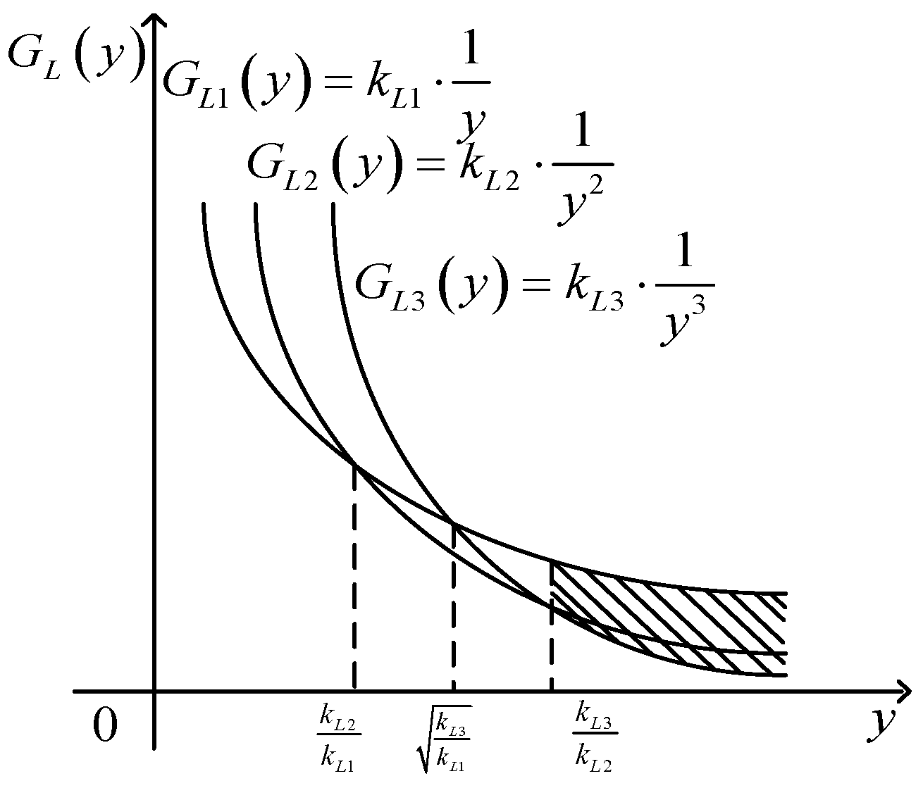
2.2. Design of the Interval for the LBC Considering Cubic Loss Expectation

When the loss of the linear term in QGLF for the LBC is $G_{L1}\left(y\right)=k_{L1}\cdot {\displaystyle \frac{1}{y}}$, the quadratic term loss is $G_{L2}\left(y\right)=k_{L2}\cdot {\displaystyle \frac{1}{y^2}}$, and the cubic term loss is $G_{L3}\left(y\right)=k_{L3}\cdot {\displaystyle \frac{1}{y^3}}$, inside the parameters $k_{L1}>0$, $k_{L2}>0$, and $k_{L3}>0$. A relationship diagram of the linear, quadratic, and cubic term losses of the QGLF for the LBC is shown in Figure 1 and Figure 2.

$G_{L1}(y)\ge G_{L2}(y)\ge G_{L3}(y)$ holds in the Taylor expansion of the QGLF. When $k_{L1}{k}_{L3}>{k_{L2}}^2$, whether to ignore the cubic loss when $G_L(y)$ is in $y\in \left({\displaystyle \frac{k_{L3}}{k_{L2}}},+\infty \right)$ is considered When $k_{L1}{k}_{L3}\le {k_{L2}}^2$, whether to ignore the cubic loss when $G_L(y)$ is in $y\in \left({\displaystyle \frac{k_{L2}}{k_{L1}}},+\infty \right)$ is considered.

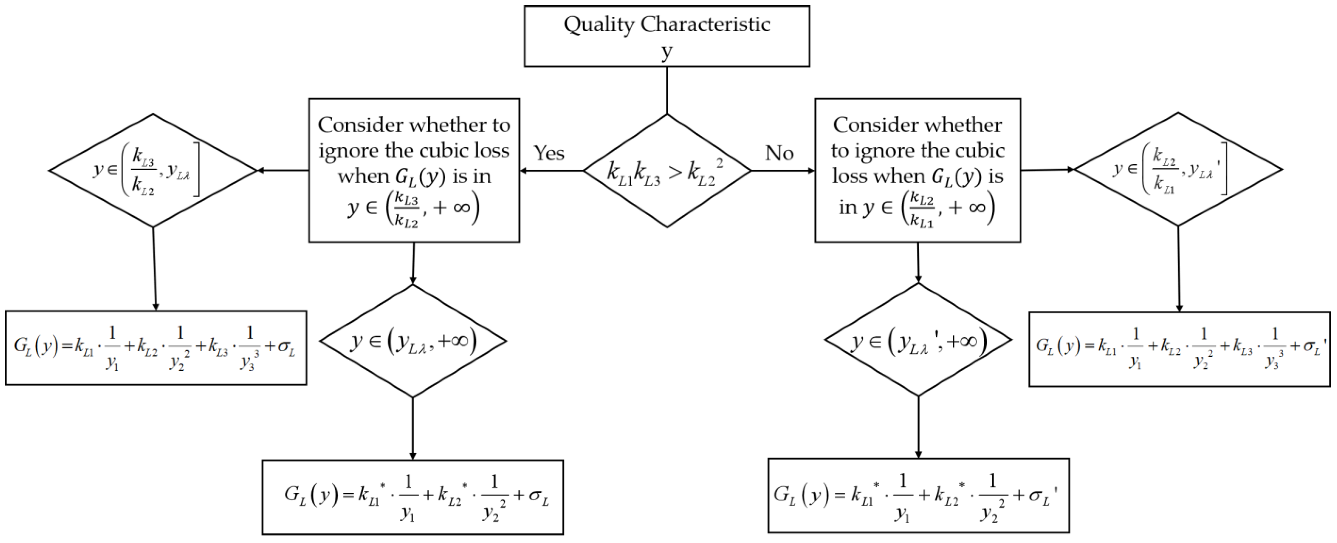
2.3. Design of QGLF for LBC Considering Cubic Loss Expectation

When considering the cubic term loss, the QGLF for the LBC is shown in Equation (3):

$$G_L\left(y\right)={\sigma }_L+k_{L1}\cdot {\displaystyle \frac{1}{y}}+k_{L2}\cdot {\displaystyle \frac{1}{y^2}}+k_{L3}\cdot {\displaystyle \frac{1}{y^3}}$$

(3)

(1) When $k_{L1}{k}_{L3}>{k_{L2}}^2$, the functional limit of the quality characteristics of the product is ${\mathsf{\Delta }}_{L0}={\phi }_L$, ${\phi }_L\in \left({\displaystyle \frac{k_{L3}}{k_{L2}}},+\infty \right)$, the quality gain–loss value is $A_{L0}$, the tolerance of the quality characteristics of the product is ${\mathsf{\Delta }}_L={\beta }_L$, ${\beta }_L\in \left({\phi }_L,+\infty \right)$, and the cost of reworking or repairing the product at this point is $A_L$. Point ${\mathsf{\Delta }}_{L1}={\gamma }_L$, ${\beta }_L<{\gamma }_L$, and ${\mathsf{\Delta }}_{L1}$ corresponds to a gain–loss of $A_{L1}$; the compensation ${\sigma }_L$ is constant.

Equation (4) can be obtained from (3) as follows:

$$\left\{\begin{array}{l}{A}_L=k_{L1}\cdot {\displaystyle \frac{1}{{\beta }_L}}+k_{L2}\cdot {\displaystyle \frac{1}{{{\beta }_L}^2}}+k_{L3}\cdot {\displaystyle \frac{1}{{{\beta }_L}^3}}+{\sigma }_L\\ A_{L0}=k_{L1}\cdot {\displaystyle \frac{1}{{\phi }_L}}+k_{L2}\cdot {\displaystyle \frac{1}{{{\phi }_L}^2}}+k_{L3}\cdot {\displaystyle \frac{1}{{{\phi }_L}^3}}+{\sigma }_L\\ A_{L1}=k_{L1}\cdot {\displaystyle \frac{1}{{\gamma }_L}}+k_{L2}\cdot {\displaystyle \frac{1}{{{\gamma }_L}^2}}+k_{L3}\cdot {\displaystyle \frac{1}{{{\gamma }_L}^3}}+{\sigma }_L\end{array}\right.$$

(4)

Equation (5) can be obtained as follows:

$$\left\{\begin{array}{c}{k}_{L1}={\displaystyle \frac{(A_L-{\sigma }_L){{\beta }_L}^3\left({\phi }_L-{\gamma }_L\right)+(A_{L1}-{\sigma }_L){{\gamma }_L}^3\left({\beta }_L-{\phi }_L\right)+(A_{L0}-{\sigma }_L){{\phi }_L}^3\left({\gamma }_L-{\beta }_L\right)}{\left({\beta }_L-{\phi }_L\right)\left({\beta }_L{\phi }_L-{\beta }_L{\gamma }_L-{\phi }_L{\gamma }_L+{{\gamma }_L}^2\right)}}\\ k_{L2}={\displaystyle \frac{(A_L-{\sigma }_L){{\beta }_L}^3\left({{\gamma }_L}^2-{{\phi }_L}^2\right)+(A_{L1}-{\sigma }_L){{\gamma }_L}^3\left({{\phi }_L}^2-{{\beta }_L}^2\right)+(A_{L0}-{\sigma }_L){{\phi }_L}^3\left({{\beta }_L}^2-{{\gamma }_L}^2\right)}{\left({\beta }_L-{\phi }_L\right)\left({\beta }_L{\phi }_L-{\beta }_L{\gamma }_L-{\phi }_L{\gamma }_L+{{\gamma }_L}^2\right)}}\\ k_{L3}={\displaystyle \frac{(A_L-{\sigma }_L){{\beta }_L}^{2}R\left({\phi }_L-{\gamma }_L\right)+(A_{L1}-{\sigma }_L){{\gamma }_L}^{2}R\left({\beta }_L-{\phi }_L\right)+(A_{L0}-{\sigma }_L){{\phi }_L}^{2}R\left({\gamma }_L-{\beta }_L\right)}{\left({\beta }_L-{\phi }_L\right)\left({\beta }_L{\phi }_L-{\beta }_L{\gamma }_L-{\phi }_L{\gamma }_L+{{\gamma }_L}^2\right)}}\end{array}\right.$$

(5)

inside $R={\beta }_L{\phi }_L{\gamma }_L$.

Substituting Equation (5) into Equation (3), we can obtain the QGLF for the LBC considering the cubic loss expectation, as shown in Equation (6):

$$\begin{array}{l}{G}_L\left(y\right)={\sigma }_L\\ +{\displaystyle \frac{(A_L-{\sigma }_L){{\beta }_L}^3\left({\phi }_L-{\gamma }_L\right)+(A_{L1}-{\sigma }_L){{\gamma }_L}^3\left({\beta }_L-{\phi }_L\right)+(A_{L0}-{\sigma }_L){{\phi }_L}^3\left({\gamma }_L-{\beta }_L\right)}{\left({\beta }_L-{\phi }_L\right)\left({\beta }_L{\phi }_L-{\beta }_L{\gamma }_L-{\phi }_L{\gamma }_L+{{\gamma }_L}^2\right)}}\cdot {\displaystyle \frac{1}{y}}\\ +{\displaystyle \frac{(A_L-{\sigma }_L){{\beta }_L}^3\left({{\gamma }_L}^2-{{\phi }_L}^2\right)+(A_{L1}-{\sigma }_L){{\gamma }_L}^3\left({{\phi }_L}^2-{{\beta }_L}^2\right)+(A_{L0}-{\sigma }_L){{\phi }_L}^3\left({{\beta }_L}^2-{{\gamma }_L}^2\right)}{\left({\beta }_L-{\phi }_L\right)\left({\beta }_L{\phi }_L-{\beta }_L{\gamma }_L-{\phi }_L{\gamma }_L+{{\gamma }_L}^2\right)}}\cdot {\displaystyle \frac{1}{y^2}}\\ +{\displaystyle \frac{(A_L-{\sigma }_L){{\beta }_L}^{2}R\left({\phi }_L-{\gamma }_L\right)+(A_{L1}-{\sigma }_L){{\gamma }_L}^{2}R\left({\beta }_L-{\phi }_L\right)+(A_{L0}-{\sigma }_L){{\phi }_L}^{2}R\left({\gamma }_L-{\beta }_L\right)}{\left({\beta }_L-{\phi }_L\right)\left({\beta }_L{\phi }_L-{\beta }_L{\gamma }_L-{\phi }_L{\gamma }_L+{{\gamma }_L}^2\right)}}\cdot {\displaystyle \frac{1}{y^3}}\end{array}$$

(6)

When $G_{L2}\left(y\right)/G_{L3}\left(y\right)={\omega }_L$, Equation (7) can be obtained as:

$$\begin{array}{c}{\displaystyle \frac{G_{L2}\left(y\right)}{G_{L3}\left(y\right)}}={\displaystyle \frac{(A_L-{\sigma }_L){{\beta }_L}^3\left({{\gamma }_L}^2-{{\phi }_L}^2\right)+(A_{L1}-{\sigma }_L){{\gamma }_L}^3\left({{\phi }_L}^2-{{\beta }_L}^2\right)+({\phi }_L-{\sigma }_L){{\phi }_L}^3\left({{\beta }_L}^2-{{\gamma }_L}^2\right)}{(A_L-{\sigma }_L){{\beta }_L}^{2}R\left({\phi }_L-{\gamma }_L\right)+(A_{L1}-{\sigma }_L){{\gamma }_L}^{2}R\left({\beta }_L-{\phi }_L\right)+(A_{L0}-{\sigma }_L){{\phi }_L}^{2}R\left({\gamma }_L-{\beta }_L\right)}}·y\\ ={\displaystyle \frac{{\left(\frac{{\gamma }_L}{{\beta }_L}\right)}^2\left[1-Q\cdot \frac{{\gamma }_L}{{\beta }_L}-P\cdot {\left(\frac{{\phi }_L}{{\beta }_L}\right)}^3\right]+{\left(\frac{{\phi }_L}{{\beta }_L}\right)}^2\left[-1+Q\cdot {\left(\frac{{\gamma }_L}{{\beta }_L}\right)}^3-P\cdot \frac{{\phi }_L}{{\beta }_L}\right]}{{\left(\frac{{\phi }_L}{{\beta }_L}\right)}^2\left[\frac{{\gamma }_L}{{\beta }_L}\left(1-P\cdot \frac{{\phi }_L}{{\beta }_L}\right)-Q·{\left(\frac{{\gamma }_L}{{\beta }_L}\right)}^3\right]+{\left(\frac{{\gamma }_L}{{\beta }_L}\right)}^2\left[\frac{{\phi }_L}{{\beta }_L}\left(-1+Q\cdot \frac{{\gamma }_L}{{\beta }_L}\right)+P·{\left(\frac{{\phi }_L}{{\beta }_L}\right)}^3\right]+\epsilon }}·{\beta }_{L}y={\omega }_L\end{array}$$

(7)

inside $P={\displaystyle \frac{A_{L0}-{\sigma }_L}{A_L-{\sigma }_L}}$ and $Q={\displaystyle \frac{A_{L1}-{\sigma }_L}{A_L-{\sigma }_L}}$.

To ensure the correctness and stability of the ratio when the denominator approached zero, we introduced an infinitesimal ε into the denominator of Equation (7) to prevent it from being too small or from being zero, thus avoiding computational instability.

Let the threshold (i.e., the critical value) for the ratio of the quadratic term loss to the cubic term loss be ${\lambda }_L={\displaystyle \frac{G_{L2}}{G_{L3}}}={\displaystyle \frac{k_{L2}}{k_{L3}}}\cdot y$. When considering the loss of the cubic term in $y\in \left({\displaystyle \frac{k_{L3}}{k_{L2}}},+\infty \right)$, we obtain ${\lambda }_L\in \left[1,+\infty \right)$. The threshold ${\lambda }_L$ is a continuous function of y.

When ${\omega }_L\in \left[1,{\lambda }_L\right]$, considering the loss of the cubic term, we can obtain Equation (8):

$$y_{L\lambda }={\displaystyle \frac{{\lambda }_L}{{\beta }_L}}·{\displaystyle \frac{{\left(\frac{{\phi }_L}{{\beta }_L}\right)}^2\left[\frac{{\gamma }_L}{{\beta }_L}\left(1-P\cdot \frac{{\phi }_L}{{\beta }_L}\right)-Q·{\left(\frac{{\gamma }_L}{{\beta }_L}\right)}^3\right]+{\left(\frac{{\gamma }_L}{{\beta }_L}\right)}^2\left[\frac{{\phi }_L}{{\beta }_L}\left(-1+Q\cdot \frac{{\gamma }_L}{{\beta }_L}\right)+P·{\left(\frac{{\phi }_L}{{\beta }_L}\right)}^3\right]}{{\left(\frac{{\gamma }_L}{{\beta }_L}\right)}^2\left[1-Q\cdot \frac{{\gamma }_L}{{\beta }_L}-P\cdot {\left(\frac{{\phi }_L}{{\beta }_L}\right)}^3\right]+{\left(\frac{{\phi }_L}{{\beta }_L}\right)}^2\left[-1+Q\cdot {\left(\frac{{\gamma }_L}{{\beta }_L}\right)}^3-P\frac{{\phi }_L}{{\beta }_L}\right]}}$$

(8)

Therefore, QGLF can be expressed as Equation (9):

$$G_L\left(y\right)=k_{L1}\cdot {\displaystyle \frac{1}{y_1}}+k_{L2}\cdot {\displaystyle \frac{1}{{y_2}^2}}+k_{L3}\cdot {\displaystyle \frac{1}{{y_3}^3}}+{\sigma }_L,y\in \left({\displaystyle \frac{k_{L3}}{k_{L2}}},y_{L\lambda }\right]$$

(9)

When $y\in \left(y_{L\lambda },+\infty \right)$, the cubic term loss is much smaller than the quadratic term loss, and thus, the cubic term loss can be neglected.

Equation (10) can be obtained from (3) as follows:

$$\left\{\begin{array}{c}{A}_L={k_{L1}}^{\ast }\cdot {\displaystyle \frac{1}{{\beta }_L}}+{k_{L2}}^{\ast }\cdot {\displaystyle \frac{1}{{{\beta }_L}^2}}+{\sigma }_L\\ A_{L0}={k_{L1}}^{\ast }\cdot {\displaystyle \frac{1}{{\phi }_L}}+{k_{L2}}^{\ast }\cdot {\displaystyle \frac{1}{{{\phi }_L}^2}}+{\sigma }_L\end{array}\right.$$

(10)

Equation (11) can be obtained as follows:

$$\left\{\begin{array}{c}{k_{L1}}^{\ast }={\displaystyle \frac{\left(A_L-{\sigma }_L\right){\mathsf{\Delta }}_L-(A_{L0}-{\sigma }_L){{\mathsf{\Delta }}_{L0}}^2}{{\mathsf{\Delta }}_L-{\mathsf{\Delta }}_{L0}}}\\ {k_{L2}}^{\ast }={\displaystyle \frac{{\mathsf{\Delta }}_L{\mathsf{\Delta }}_{L0}\left[\left(A_{L0}-{\sigma }_L\right){\mathsf{\Delta }}_{L0}-\left(A_L-{\sigma }_L\right){\mathsf{\Delta }}_L\right]}{{\mathsf{\Delta }}_L-{\mathsf{\Delta }}_{L0}}}\end{array}\right.$$

(11)

Therefore, QGLF can be expressed as Equation (12):

$$G_L\left(y\right)={k_{L1}}^{\ast }\cdot {\displaystyle \frac{1}{y_1}}+{k_{L2}}^{\ast }\cdot {\displaystyle \frac{1}{{y_2}^2}}+{\sigma }_L,y\in \left(y_{L\lambda },+\infty \right]$$

(12)

Therefore, when $k_{L1}{k}_{L3}>{k_{L2}}^2$, QGLF can be expressed as Equation (13):

$$\left\{\begin{array}{c}{G}_L\left(y\right)=k_{L1}\cdot {\displaystyle \frac{1}{y_1}}+k_{L2}\cdot {\displaystyle \frac{1}{{y_2}^2}}+k_{L3}\cdot {\displaystyle \frac{1}{{y_3}^3}}+{\sigma }_L,y\in \left({\displaystyle \frac{k_{L3}}{k_{L2}}},y_{L\lambda }\right]\\ G_L\left(y\right)={k_{L1}}^{\ast }\cdot {\displaystyle \frac{1}{y_1}}+{k_{L2}}^{\ast }\cdot {\displaystyle \frac{1}{{y_2}^2}}+{\sigma }_L,y\in \left(y_{L\lambda },+\infty \right)\end{array}\right.$$

(13)

(2) When $k_{L1}{k}_{L3}\le {k_{L2}}^2$, the functional limit of the quality characteristics of the product is ${{\mathsf{\Delta }}_{L0}}^{\prime }={{\phi }_L}^{\prime }$, ${{\phi }_L}^{\prime }\in \left({\displaystyle \frac{k_{L2}}{k_{L1}}},+\infty \right)$, and the quality gain–loss value is ${A_{L0}}^{\prime }$, the tolerance of the quality characteristics of the product is ${{\mathsf{\Delta }}_L}^{\prime }={{\beta }_L}^{\prime }$, ${{\beta }_L}^{\prime }\in \left({{\phi }_L}^{\prime },+\infty \right)$, and the cost of reworking or repairing the product at this point is ${A_L}^{\prime }$. When Point ${{\mathsf{\Delta }}_{L1}}^{\prime }={{\gamma }_L}^{\prime }$, ${{\beta }_L}^{\prime }<{{\gamma }_L}^{\prime }$, ${{\mathsf{\Delta }}_{L1}}^{\prime }$ corresponds to a gain–loss of ${A_{L1}}^{\prime }$; the compensation ${{\sigma }_L}^{\prime }$ is constant.

Equation (14) can be obtained from (3) as follows:

$$\left\{\begin{array}{l}{A_L}^{\prime }={k_{L1}}^{\prime }\cdot {\displaystyle \frac{1}{{{\beta }_L}^{\prime }}}+{k_{L2}}^{\prime }\cdot {\displaystyle \frac{1}{{{\beta }_L}^{\prime 2}}}+{k_{L3}}^{\prime }\cdot {\displaystyle \frac{1}{{{\beta }_L}^{\prime 3}}}+{{\sigma }_L}^{\prime }\\ {A_{L0}}^{\prime }={k_{L1}}^{\prime }\cdot {\displaystyle \frac{1}{{{\phi }_L}^{\prime }}}+{k_{L2}}^{\prime }\cdot {\displaystyle \frac{1}{{{\phi }_L}^{\prime 2}}}+{k_{L3}}^{\prime }\cdot {\displaystyle \frac{1}{{{\phi }_L}^{\prime 3}}}+{{\sigma }_L}^{\prime }\\ {A_{L1}}^{\prime }={k_{L1}}^{\prime }\cdot {\displaystyle \frac{1}{{{\gamma }_L}^{\prime }}}+{k_{L2}}^{\prime }\cdot {\displaystyle \frac{1}{{{\gamma }_L}^{\prime 2}}}+{k_{L3}}^{\prime }\cdot {\displaystyle \frac{1}{{{\gamma }_L}^{\prime 3}}}+{{\sigma }_L}^{\prime }\end{array}\right.$$

(14)

Equation (15) can be obtained as:

$$\left\{\begin{array}{c}{k_{L1}}^{\prime }={\displaystyle \frac{({A_L}^{\prime }-{{\sigma }_L}^{\prime }){{\beta }_L}^{\prime 3}\left({{\phi }_L}^{\prime }-{{\gamma }_L}^{\prime }\right)+({A_{L1}}^{\prime }-{{\sigma }_L}^{\prime }){{\gamma }_L}^{\prime 3}\left({{\beta }_L}^{\prime }-{{\phi }_L}^{\prime }\right)+({A_{L0}}^{\prime }-{{\sigma }_L}^{\prime }){{\phi }_L}^{\prime 3}\left({{\gamma }_L}^{\prime }-{{\beta }_L}^{\prime }\right)}{\left({\beta }_L-{\phi }_L\right)\left({\beta }_L{\phi }_L-{\beta }_L{\gamma }_L-{\phi }_L{\gamma }_L+{{\gamma }_L}^2\right)}}\\ {k_{L2}}^{\prime }={\displaystyle \frac{({A_L}^{\prime }-{{\sigma }_L}^{\prime }){{\beta }_L}^{\prime 3}\left({{\gamma }_L}^{\prime 2}-{{\phi }_L}^{\prime 2}\right)+({A_{L1}}^{\prime }-{{\sigma }_L}^{\prime }){{\gamma }_L}^{\prime 3}\left({{\phi }_L}^{\prime 2}-{{\beta }_L}^{\prime 2}\right)+({A_{L0}}^{\prime }-{{\sigma }_L}^{\prime }){{\phi }_L}^{\prime 3}\left({{\beta }_L}^{\prime 2}-{{\gamma }_L}^{\prime 2}\right)}{\left({\beta }_L-{\phi }_L\right)\left({\beta }_L{\phi }_L-{\beta }_L{\gamma }_L-{\phi }_L{\gamma }_L+{{\gamma }_L}^2\right)}}\\ {k_{L3}}^{\prime }={\displaystyle \frac{({A_L}^{\prime }-{{\sigma }_L}^{\prime }){{\beta }_L}^{\prime 2}{R}^{\prime }\left({{\phi }_L}^{\prime }-{{\gamma }_L}^{\prime }\right)+({A_{L1}}^{\prime }-{{\sigma }_L}^{\prime }){{\gamma }_L}^{\prime 2}{R}^{\prime }\left({{\beta }_L}^{\prime }-{{\phi }_L}^{\prime }\right)+({A_{L0}}^{\prime }-{{\sigma }_L}^{\prime }){{\phi }_L}^{\prime 2}{R}^{\prime }\left({{\gamma }_L}^{\prime }-{{\beta }_L}^{\prime }\right)}{\left({{\beta }_L}^{\prime }-{{\phi }_L}^{\prime }\right)\left({{\beta }_L}^{\prime }{{\phi }_L}^{\prime }-{{\beta }_L}^{\prime }{{\gamma }_L}^{\prime }-{{\phi }_L}^{\prime }{{\gamma }_L}^{\prime }+{{\gamma }_L}^{\prime 2}\right)}}\end{array}\right.$$

(15)

inside $R^{\prime }={{\beta }_L}^{\prime }{{\phi }_L}^{\prime }{{\gamma }_L}^{\prime }$.

Substituting Equation (15) into Equation (3), we can obtain the QGLF for the LBC considering the cubic loss expectation, as shown in Equation (16):

$$\begin{array}{l}{G_L}^{\prime }\left(y\right)={{\sigma }_L}^{\prime }\\ +{\displaystyle \frac{({A_L}^{\prime }-{{\sigma }_L}^{\prime }){{\beta }_L}^{\prime 3}\left({{\phi }_L}^{\prime }-{{\gamma }_L}^{\prime }\right)+({A_{L1}}^{\prime }-{{\sigma }_L}^{\prime }){{\gamma }_L}^{\prime 3}\left({{\beta }_L}^{\prime }-{{\phi }_L}^{\prime }\right)+({A_{L0}}^{\prime }-{{\sigma }_L}^{\prime }){{\phi }_L}^{\prime 3}\left({{\gamma }_L}^{\prime }-{{\beta }_L}^{\prime }\right)}{\left({{\beta }_L}^{\prime }-{{\phi }_L}^{\prime }\right)\left({{\beta }_L}^{\prime }{{\phi }_L}^{\prime }-{{\beta }_L}^{\prime }{{\gamma }_L}^{\prime }-{{\phi }_L}^{\prime }{{\gamma }_L}^{\prime }+{{\gamma }_L}^{\prime 2}\right)}}\cdot {\displaystyle \frac{1}{y}}\\ +{\displaystyle \frac{({A_L}^{\prime }-{{\sigma }_L}^{\prime }){{\beta }_L}^{\prime 3}\left({{\gamma }_L}^{\prime 2}-{{\phi }_L}^{\prime 2}\right)+({A_{L1}}^{\prime }-{{\sigma }_L}^{\prime }){{\gamma }_L}^{\prime 3}\left({{\phi }_L}^{\prime 2}-{{\beta }_L}^{\prime 2}\right)+({A_{L0}}^{\prime }-{{\sigma }_L}^{\prime }){{\phi }_L}^{\prime 3}\left({{\beta }_L}^{\prime 2}-{{\gamma }_L}^{\prime 2}\right)}{\left({\beta }_L-{\phi }_L\right)\left({\beta }_L{\phi }_L-{\beta }_L{\gamma }_L-{\phi }_L{\gamma }_L+{{\gamma }_L}^2\right)}}\\ \cdot {\displaystyle \frac{1}{y^2}}+{\displaystyle \frac{({A_L}^{\prime }-{{\sigma }_L}^{\prime }){{\beta }_L}^{\prime 2}{R}^{\prime }\left({{\phi }_L}^{\prime }-{{\gamma }_L}^{\prime }\right)+({A_{L1}}^{\prime }-{{\sigma }_L}^{\prime }){{\gamma }_L}^{\prime 2}{R}^{\prime }\left({{\beta }_L}^{\prime }-{{\phi }_L}^{\prime }\right)+({A_{L0}}^{\prime }-{{\sigma }_L}^{\prime }){{\phi }_L}^{\prime 2}{R}^{\prime }\left({{\gamma }_L}^{\prime }-{{\beta }_L}^{\prime }\right)}{\left({{\beta }_L}^{\prime }-{{\phi }_L}^{\prime }\right)\left({{\beta }_L}^{\prime }{{\phi }_L}^{\prime }-{{\beta }_L}^{\prime }{{\gamma }_L}^{\prime }-{{\phi }_L}^{\prime }{{\gamma }_L}^{\prime }+{{\gamma }_L}^{\prime 2}\right)}}\cdot {\displaystyle \frac{1}{y^3}}\end{array}$$

(16)

When $G_{L2}\left(y\right)/G_{L3}\left(y\right)={{\omega }_L}^{\prime }$, Equation (17) can be obtained as:

$$\begin{array}{l}{\displaystyle \frac{G_{L2}\left(y\right)}{G_{L3}\left(y\right)}}\\ ={\displaystyle \frac{({A_L}^{\prime }-{\sigma }_L){{\beta }_L}^{\prime 3}\left({{\gamma }_L}^{\prime 2}-{{\phi }_L}^{\prime 2}\right)+({A_{L1}}^{\prime }-{\sigma }_L){{\gamma }_L}^{\prime 3}\left({{\phi }_L}^{\prime 2}-{{\beta }_L}^{\prime 2}\right)+({A_{L0}}^{\prime }-{\sigma }_L){{\phi }_L}^{\prime 3}\left({{\beta }_L}^{\prime 2}-{{\gamma }_L}^{\prime 2}\right)}{({A_L}^{\prime }-{\sigma }_L){{\beta }_L}^{\prime }\left({{\phi }_L}^{\prime }-{{\gamma }_L}^{\prime }\right)+({A_{L1}}^{\prime }-{\sigma }_L){{\gamma }_L}^{\prime }\left({{\beta }_L}^{\prime }-{{\phi }_L}^{\prime }\right)+({A_{L0}}^{\prime }-{\sigma }_L){{\phi }_L}^{\prime }\left({{\gamma }_L}^{\prime }-{{\beta }_L}^{\prime }\right)}}\cdot y\\ ={\displaystyle \frac{{\left(\frac{{{\gamma }_L}^{\prime }}{{{\beta }_L}^{\prime }}\right)}^2\left[1-Q^{\prime }\cdot \frac{{{\gamma }_L}^{\prime }}{{{\beta }_L}^{\prime }}-P^{\prime }\cdot {\left(\frac{{{\phi }_L}^{\prime }}{{{\beta }_L}^{\prime }}\right)}^3\right]+{\left(\frac{{{\phi }_L}^{\prime }}{{{\beta }_L}^{\prime }}\right)}^2\left[-1+Q^{\prime }\cdot {\left(\frac{{{\gamma }_L}^{\prime }}{{{\beta }_L}^{\prime }}\right)}^3-P^{\prime }\cdot \frac{{{\phi }_L}^{\prime }}{{{\beta }_L}^{\prime }}\right]}{{\left(\frac{{{\phi }_L}^{\prime }}{{{\beta }_L}^{\prime }}\right)}^2\left[\frac{{{\gamma }_L}^{\prime }}{{{\beta }_L}^{\prime }}\left(1-P^{\prime }\cdot \frac{{{\phi }_L}^{\prime }}{{{\beta }_L}^{\prime }}\right)-Q^{\prime }\cdot {\left(\frac{{{\gamma }_L}^{\prime }}{{{\beta }_L}^{\prime }}\right)}^3\right]+{\left(\frac{{{\gamma }_L}^{\prime }}{{{\beta }_L}^{\prime }}\right)}^2\left[\frac{{{\phi }_L}^{\prime }}{{{\beta }_L}^{\prime }}\left(-1+Q^{\prime }\cdot \frac{{{\gamma }_L}^{\prime }}{{{\beta }_L}^{\prime }}\right)+P^{\prime }\cdot {\left(\frac{{{\phi }_L}^{\prime }}{{{\beta }_L}^{\prime }}\right)}^3\right]+\epsilon }}\cdot {{\beta }_L}^{\prime }y={{\omega }_L}^{\prime }\end{array}$$

(17)

inside $P^{\prime }={\displaystyle \frac{{A_{L0}}^{\prime }-{{\sigma }_L}^{\prime }}{{A_L}^{\prime }-{{\sigma }_L}^{\prime }}}$ and $Q^{\prime }={\displaystyle \frac{{A_{L1}}^{\prime }-{{\sigma }_L}^{\prime }}{{A_L}^{\prime }-{{\sigma }_L}^{\prime }}}$.

To ensure the correctness and stability of the ratio when the denominator approached zero, we introduced an infinitesimal ε into the denominator of Equation (17) to prevent it from being too small or zero, thus avoiding computational instability.

Let the threshold (i.e., the critical value) for the ratio of the quadratic term loss to the cubic term loss be ${{\lambda }_L}^{\prime }={\displaystyle \frac{G_{L2}}{G_{L3}}}={\displaystyle \frac{k_{L2}}{k_{L3}}}\cdot y$. When considering the loss of the cubic term as being $y\in \left({\displaystyle \frac{k_{L3}}{k_{L2}}},+\infty \right)$, we can obtain ${{\lambda }_L}^{\prime }\in \left[1,+\infty \right)$.

When ${{\omega }_L}^{\prime }\in \left[1,{{\lambda }_L}^{\prime }\right]$, considering the loss of the cubic term, we can obtain Equation (18):

$${y_{L\lambda }}^{\prime }={\displaystyle \frac{{\left(\frac{{{\phi }_L}^{\prime }}{{{\beta }_L}^{\prime }}\right)}^2\left[\frac{{{\gamma }_L}^{\prime }}{{{\beta }_L}^{\prime }}\left(1-P^{\prime }\cdot \frac{{{\phi }_L}^{\prime }}{{{\beta }_L}^{\prime }}\right)-Q^{\prime }·{\left(\frac{{{\gamma }_L}^{\prime }}{{{\beta }_L}^{\prime }}\right)}^3\right]+{\left(\frac{{{\gamma }_L}^{\prime }}{{{\beta }_L}^{\prime }}\right)}^2\left[\frac{{{\phi }_L}^{\prime }}{{{\beta }_L}^{\prime }}\left(-1+Q^{\prime }\cdot \frac{{{\gamma }_L}^{\prime }}{{{\beta }_L}^{\prime }}\right)+P^{\prime }·{\left(\frac{{{\phi }_L}^{\prime }}{{{\beta }_L}^{\prime }}\right)}^3\right]}{{\left(\frac{{{\gamma }_L}^{\prime }}{{{\beta }_L}^{\prime }}\right)}^2\left[1-Q^{\prime }\cdot \frac{{{\gamma }_L}^{\prime }}{{{\beta }_L}^{\prime }}-P^{\prime }\cdot {\left(\frac{{{\phi }_L}^{\prime }}{{{\beta }_L}^{\prime }}\right)}^3\right]+{\left(\frac{{{\phi }_L}^{\prime }}{{{\beta }_L}^{\prime }}\right)}^2\left[-1+Q^{\prime }\cdot {\left(\frac{{{\gamma }_L}^{\prime }}{{{\beta }_L}^{\prime }}\right)}^3-P^{\prime }\cdot \frac{{{\phi }_L}^{\prime }}{{{\beta }_L}^{\prime }}\right]}}·{\displaystyle \frac{{{\lambda }_L}^{\prime }}{{{\beta }_L}^{\prime }}}$$

(18)

Therefore, QGLF can be expressed as Equation (19):

$$G_L\left(y\right)=k_{L1}\cdot {\displaystyle \frac{1}{y_1}}+k_{L2}\cdot {\displaystyle \frac{1}{{y_2}^2}}+k_{L3}\cdot {\displaystyle \frac{1}{{y_3}^3}}+{{\sigma }_L}^{\prime },y\in \left({\displaystyle \frac{k_{L2}}{k_{L1}}},{y_{L\lambda }}^{\prime }\right]$$

(19)

When $y\in \left({y_{L\lambda }}^{\prime },+\infty \right)$, the cubic term loss is much smaller than the quadratic term loss, and thus, the cubic term loss can be neglected.

Equation (20) can be obtained from Equation (3) as follows:

$$\left\{\begin{array}{c}{A_L}^{\prime }={k_{L1}}^{\ast }\cdot {\displaystyle \frac{1}{{{\beta }_L}^{\prime }}}+{k_{L2}}^{\ast }\cdot {\displaystyle \frac{1}{{{\beta }_L}^{\prime 2}}}+{{\sigma }_L}^{\prime }\\ {A_{L0}}^{\prime }={k_{L1}}^{\ast }\cdot {\displaystyle \frac{1}{{{\phi }_L}^{\prime }}}+{k_{L2}}^{\ast }\cdot {\displaystyle \frac{1}{{{\phi }_L}^{\prime 2}}}+{{\sigma }_L}^{\prime }\end{array}\right.$$

(20)

Equation (21) is obtained as follows:

$$\left\{\begin{array}{c}{k_{L1}}^{\ast }={\displaystyle \frac{\left({A_L}^{\prime }-{{\sigma }_L}^{\prime }\right){{\mathsf{\Delta }}_L}^{\prime }-({A_{L0}}^{\prime }-{{\sigma }_L}^{\prime }){{\mathsf{\Delta }}_{L0}^{\prime }}^2}{{\mathsf{\Delta }}_L-{\mathsf{\Delta }}_{L0}}}\\ {k_{L2}}^{\ast }={\displaystyle \frac{{{\mathsf{\Delta }}_L}^{\prime }{{\mathsf{\Delta }}_{L0}}^{\prime }\left[\left({A_{L0}}^{\prime }-{{\sigma }_L}^{\prime }\right){\mathsf{\Delta }}_{L0}^{\prime }-\left({A_L}^{\prime }-{{\sigma }_L}^{\prime }\right){{\mathsf{\Delta }}_L}^{\prime }\right]}{{{\mathsf{\Delta }}_L}^{\prime }-{{\mathsf{\Delta }}_{L0}}^{\prime }}}\end{array}\right.$$

(21)

Therefore, QGLF can be expressed as Equation (22):

$$G_L\left(y\right)={k_{L1}}^{\ast }\cdot {\displaystyle \frac{1}{y_1}}+{k_{L2}}^{\ast }\cdot {\displaystyle \frac{1}{{y_2}^2}}+{{\sigma }_L}^{\prime },y\in \left({y_{L\lambda }}^{\prime },+\infty \right]$$

(22)

Therefore, when $k_{L1}{k}_{L3}\le {k_{L2}}^2$, QGLF can be expressed as Equation (23):

$$\left\{\begin{array}{c}{G}_L\left(y\right)=k_{L1}\cdot {\displaystyle \frac{1}{y_1}}+k_{L2}\cdot {\displaystyle \frac{1}{{y_2}^2}}+k_{L3}\cdot {\displaystyle \frac{1}{{y_3}^3}}+{{\sigma }_L}^{\prime },y\in \left({\displaystyle \frac{k_{L2}}{k_{L1}}},{y_{L\lambda }}^{\prime }\right]\\ G_L\left(y\right)={k_{L1}}^{\ast }\cdot {\displaystyle \frac{1}{y_1}}+{k_{L2}}^{\ast }\cdot {\displaystyle \frac{1}{{y_2}^2}}+{{\sigma }_L}^{\prime },y\in \left({y_{L\lambda }}^{\prime },+\infty \right)\end{array}\right.$$

(23)

The flow chart of the QGLF for the LBC is shown in Figure 3.

3. Design of the QGLF for the SBC Considering Cubic Loss Expectation

3.1. QGLF for SBC

$G_S\left(y\right)$ represents the QGLF for the SBC, and a Taylor series expansion at $y=0$ yields Equation (24) as follows:

$$G_S\left(y\right)=G_S\left(0\right)+{\displaystyle \frac{{G^{\prime }}_S\left(0\right)}{1!}}\cdot y+{\displaystyle \frac{{G^{″}}_S\left(0\right)}{2!}}\cdot y^2+{\displaystyle \frac{{G^{‴}}_S\left(0\right)}{3!}}\cdot y^3+R_3\left(y\right)$$

(24)

Inside $R_3\left(y\right)$ is the truncation error, expressed as $R_3\left(y\right)={\displaystyle \frac{{G^{\left(4\right)}}_S\left(\xi \right)}{4!}}\cdot y^4$, and $\xi$ is a point between 0 and y.

Here, $R_3\left(y\right)={\displaystyle \frac{{G^{\left(4\right)}}_S\left(\xi \right)}{4!}}\cdot y^4$ represents the truncation error introduced by neglecting higher-order terms in the Taylor series expansion. Since y is typically small in the QGLF for the SBC, the term $y^4$ ensures that the truncation error remains small and does not significantly affect the accuracy of the method.

Assuming constant mass compensation, i.e., $G_S\left(0\right)={\sigma }_{S0}$, ${\sigma }_{S0}\in R$ and ${G^{\prime }}_S\left(0\right)=0$, neglecting the terms above the quadratic term in the Taylor expansion, Equation (25) can be obtained:

$$G_S\left(y\right)={\sigma }_{S0}+k_S\cdot y^2,y\in \left(0,+\infty \right)$$

(25)

3.2. Design of the Interval for the SBC Considering Cubic Loss Expectation

When the loss of the linear term in the QGLF for SBC is $G_{S1}\left(y\right)=k_{S1}\cdot y$, the quadratic term loss is $G_{S2}\left(y\right)=k_{S2}\cdot y^2$, and the cubic term loss is $G_{S3}\left(y\right)=k_{S3}\cdot y^3$, inside the parameters $k_{S1}>0$, $k_{S2}>0$, and $k_{S3}>0$. A relationship diagram of the linear, quadratic, and cubic term losses of the QGLF for the SBC is shown in Figure 4 and Figure 5.

$G_{S1}(y)\ge G_{S2}(y)\ge G_{S3}(y)$ holds in the Taylor expansion of the QGLF. When $k_{S1}{k}_{S3}>{k_{S2}}^2$, whether to ignore the cubic loss when $G_S(y)$ is in $y\in \left(0,{\displaystyle \frac{k_{S2}}{k_{S3}}}\right)$ is considered. When $k_{S1}{k}_{S3}\le {k_{S2}}^2$, whether to ignore the cubic loss when $G_S(y)$ is in $y\in \left(0,{\displaystyle \frac{k_{S1}}{k_{S2}}}\right)$ is considered.

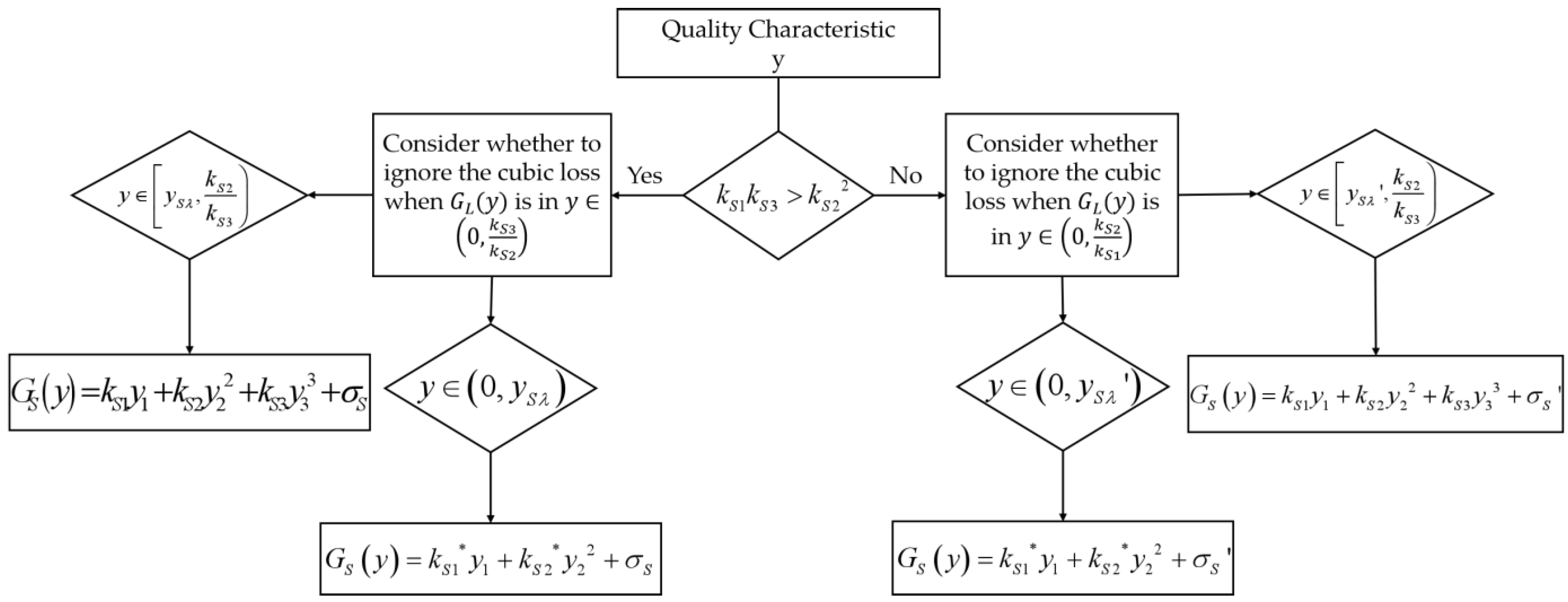
3.3. Design of the QGLF for the SBC Considering Cubic Loss Expectation

When considering the cubic term loss, the QGLF for the SBC can be obtained using Equation (26):

$$G_S\left(y\right)={\sigma }_S+k_{S1}\cdot y+k_{S2}\cdot y^2+k_{S3}\cdot y^3$$

(26)

(1) When $k_{S1}{k}_{S3}>{k_{S2}}^2$, the functional limit of the qualities characteristics of the product is ${\mathsf{\Delta }}_{S0}={\phi }_S$, ${\phi }_S\in \left(0,{\displaystyle \frac{k_{S2}}{k_{S3}}}\right)$, and the quality gain–loss value is $A_{S0}$. The tolerance of the quality characteristics of the product is ${\mathsf{\Delta }}_S={\beta }_S$, ${\beta }_S\in \left(0,{\phi }_S\right)$, and the cost of reworking or repairing the product at this point is $A_S$. When point ${\mathsf{\Delta }}_{S1}={\gamma }_S$, $0<{\gamma }_S<{\beta }_S<{\phi }_S$, ${\mathsf{\Delta }}_{S1}$ corresponds to a gain–loss of $A_{S1}$; the compensation ${\sigma }_S$ is constant.

Equation (27) can be obtained from Equation (26) as follows:

$$\left\{\begin{array}{l}{A}_S=k_{S1}\cdot {\beta }_S+k_{S2}\cdot {{\beta }_S}^2+k_{S3}\cdot {{\beta }_S}^3+{\sigma }_S\\ A_{S0}=k_{S1}\cdot {\phi }_S+k_{S2}\cdot {{\phi }_S}^2+k_{S3}\cdot {{\phi }_S}^3+{\sigma }_S\\ A_{S1}=k_{S1}\cdot {\gamma }_S+k_{S2}\cdot {{\gamma }_S}^2+k_{S3}\cdot {{\gamma }_S}^3+{\sigma }_S\end{array}\right.$$

(27)

Equation (28) is shown as follows:

$$\left\{\begin{array}{l}{k}_{S1}={\displaystyle \frac{\left(A_{S1}-{\sigma }_S\right)\left({{\phi }_S}^3{{\beta }_S}^2-{{\phi }_S}^2{{\beta }_S}^3\right)+\left(A_{S0}-{\sigma }_S\right)\left({{\gamma }_S}^2{{\beta }_S}^3-{{\gamma }_S}^3{{\beta }_S}^2\right)+\left(A_S-{\sigma }_S\right)\left({{\gamma }_S}^3{{\phi }_S}^2-{{\gamma }_S}^2{{\phi }_S}^3\right)}{{\gamma }_S{\phi }_S{\beta }_S\left({\gamma }_S-{\beta }_S\right)\left({\phi }_S-{\beta }_S\right)\left({\gamma }_S-{\phi }_S\right)}}\\ k_{S2}={\displaystyle \frac{\left(A_{S1}-{\sigma }_S\right)\left({\phi }_S{{\beta }_S}^3-{{\phi }_S}^3{\beta }_S\right)+\left(A_{S0}-{\sigma }_S\right)\left({{\gamma }_S}^3{\beta }_S-{\gamma }_S{{\beta }_S}^3\right)+\left(A_S-{\sigma }_S\right)\left({\gamma }_S{{\phi }_S}^3-{{\gamma }_S}^3{\phi }_S\right)}{{\gamma }_S{\phi }_S{\beta }_S\left({\gamma }_S-{\beta }_S\right)\left({\phi }_S-{\beta }_S\right)\left({\gamma }_S-{\phi }_S\right)}}\\ k_{S3}={\displaystyle \frac{\left(A_{S1}-{\sigma }_S\right)\left({{\phi }_S}^2{\beta }_S-{\phi }_S{{\beta }_S}^2\right)+\left(A_{S0}-{\sigma }_S\right)\left({\gamma }_S{{\beta }_S}^2-{{\gamma }_S}^2{\beta }_S\right)+\left(A_S-{\sigma }_S\right)\left({{\gamma }_S}^2{\phi }_S-{\gamma }_S{{\phi }_S}^2\right)}{{\gamma }_S{\phi }_S{\beta }_S\left({\gamma }_S-{\beta }_S\right)\left({\phi }_S-{\beta }_S\right)\left({\gamma }_S-{\phi }_S\right)}}\end{array}\right.$$

(28)

By substituting Equation (28) into Equation (26), we can obtain the QGLF for the SBC considering cubic loss expectation, as shown in Equation (29):

$$\begin{array}{l}{G}_S\left(y\right)={\sigma }_S\\ +{\displaystyle \frac{\left(A_{S1}-{\sigma }_S\right)\left({{\phi }_S}^3{{\beta }_S}^2-{{\phi }_S}^2{{\beta }_S}^3\right)+\left(A_{S0}-{\sigma }_S\right)\left({{\gamma }_S}^2{{\beta }_S}^3-{{\gamma }_S}^3{{\beta }_S}^2\right)+\left(A_S-{\sigma }_S\right)\left({{\gamma }_S}^3{{\phi }_S}^2-{{\gamma }_S}^2{{\phi }_S}^3\right)}{{\gamma }_S{\phi }_S{\beta }_S\left({\gamma }_S-{\beta }_S\right)\left({\phi }_S-{\beta }_S\right)\left({\gamma }_S-{\phi }_S\right)}}\cdot y\\ +{\displaystyle \frac{\left(A_{S1}-{\sigma }_S\right)\left({\phi }_S{{\beta }_S}^3-{{\phi }_S}^3{\beta }_S\right)+\left(A_{S0}-{\sigma }_S\right)\left({{\gamma }_S}^3{\beta }_S-{\gamma }_S{{\beta }_S}^3\right)+\left(A_S-{\sigma }_S\right)\left({\gamma }_S{{\phi }_S}^3-{{\gamma }_S}^3{\phi }_S\right)}{{\gamma }_S{\phi }_S{\beta }_S\left({\gamma }_S-{\beta }_S\right)\left({\phi }_S-{\beta }_S\right)\left({\gamma }_S-{\phi }_S\right)}}\cdot y^2\\ +{\displaystyle \frac{\left(A_{S1}-{\sigma }_S\right)\left({{\phi }_S}^2{\beta }_S-{\phi }_S{{\beta }_S}^2\right)+\left(A_{S0}-{\sigma }_S\right)\left({\gamma }_S{{\beta }_S}^2-{{\gamma }_S}^2{\beta }_S\right)+\left(A_S-{\sigma }_S\right)\left({{\gamma }_S}^2{\phi }_S-{\gamma }_S{{\phi }_S}^2\right)}{{\gamma }_S{\phi }_S{\beta }_S\left({\gamma }_S-{\beta }_S\right)\left({\phi }_S-{\beta }_S\right)\left({\gamma }_S-{\phi }_S\right)}}\cdot y^3\end{array}$$

(29)

When $G_{S2}\left(y\right)/G_{S3}\left(y\right)={\omega }_S$, Equation (30) is as follows:

$$\begin{array}{l}{\displaystyle \frac{G_{S2}\left(y\right)}{G_{S3}\left(y\right)}}\\ ={\displaystyle \frac{\left(A_{S1}-{\sigma }_S\right)\left({\phi }_S{{\beta }_S}^3-{{\phi }_S}^3{\beta }_S\right)+\left(A_{S0}-{\sigma }_S\right)\left({{\gamma }_S}^3{\beta }_S-{\gamma }_S{{\beta }_S}^3\right)+\left(A_S-{\sigma }_S\right)\left({\gamma }_S{{\phi }_S}^3-{{\gamma }_S}^3{\phi }_S\right)}{\left(A_{S1}-{\sigma }_S\right)\left({{\phi }_S}^2{\beta }_S-{\phi }_S{{\beta }_S}^2\right)+\left(A_{S0}-{\sigma }_S\right)\left({\gamma }_S{{\beta }_S}^2-{{\gamma }_S}^2{\beta }_S\right)+\left(A_S-{\sigma }_S\right)\left({{\gamma }_S}^2{\phi }_S-{\gamma }_S{{\phi }_S}^2\right)}}·{\displaystyle \frac{1}{y}}\\ ={\displaystyle \frac{\frac{{\phi }_S}{{\beta }_S}\left\{\frac{A_{S1}-{\sigma }_S}{A_S-{\sigma }_S}\left[1-{\left(\frac{{\phi }_S}{{\beta }_S}\right)}^2\right]+\frac{{\gamma }_S}{{\beta }_S}{\left(\frac{{\phi }_S}{{\beta }_S}\right)}^2\right\}-\frac{{\gamma }_S}{{\beta }_S}\left\{\frac{A_{S0}-{\sigma }_S}{A_S-{\sigma }_S}\left[1-{\left(\frac{{\gamma }_S}{{\beta }_S}\right)}^2\right]+{\left(\frac{{\gamma }_S}{{\beta }_S}\right)}^2\frac{{\phi }_S}{{\beta }_S}\right\}}{\frac{{\phi }_S}{{\beta }_S}\left[-\frac{A_{S1}-{\sigma }_S}{A_S-{\sigma }_S}\left(1-\frac{{\phi }_S}{{\beta }_S}\right)-\frac{{\gamma }_S}{{\beta }_S}\cdot \frac{{\phi }_S}{{\beta }_S}\right]+\frac{{\gamma }_S}{{\beta }_S}\left[\frac{A_{S0}-{\sigma }_S}{A_S-{\sigma }_S}\left(1-\frac{{\gamma }_S}{{\beta }_S}\right)+\frac{{\gamma }_S}{{\beta }_S}\cdot \frac{{\phi }_S}{{\beta }_S}\right]+\epsilon }}\cdot {\displaystyle \frac{{\beta }_S}{y}}={\omega }_S\end{array}$$

(30)

To ensure the correctness and stability of the ratio when the denominator approached zero, we introduced an infinitesimal ε into the denominator of Equation (30) to prevent it from being too small or zero, thus avoiding computational instability.

Let the threshold (i.e., the critical value) for the ratio of the quadratic term loss to the cubic term loss be ${\lambda }_S={\displaystyle \frac{G_{S2}}{G_{S3}}}={\displaystyle \frac{k_{S2}}{k_{S3}}}\cdot {\displaystyle \frac{1}{y}}$. When considering the loss of the cubic term in $y\in \left(0,{\displaystyle \frac{k_{S2}}{k_{S3}}}\right)$, we can obtain ${\lambda }_S\in \left[1,+\infty \right)$.

When ${\omega }_S\in \left[1,{\lambda }_S\right]$, considering the loss of the cubic term, we can obtain Equation (31):

$$y_{S\lambda }={\displaystyle \frac{\frac{{\phi }_S}{{\beta }_S}\left\{\frac{A_{S1}-{\sigma }_S}{A_S-{\sigma }_S}\left[1-{\left(\frac{{\phi }_S}{{\beta }_S}\right)}^2\right]+\frac{{\gamma }_S}{{\beta }_S}{\left(\frac{{\phi }_S}{{\beta }_S}\right)}^2\right\}-\frac{{\gamma }_S}{{\beta }_S}\left\{\frac{A_{S0}-{\sigma }_S}{A_S-{\sigma }_S}\left[1-{\left(\frac{{\gamma }_S}{{\beta }_S}\right)}^2\right]+{\left(\frac{{\gamma }_S}{{\beta }_S}\right)}^2\frac{{\phi }_S}{{\beta }_S}\right\}}{\frac{{\phi }_S}{{\beta }_S}\left[-\frac{A_{S1}-{\sigma }_S}{A_S-{\sigma }_S}\left(1-\frac{{\phi }_S}{{\beta }_S}\right)-\frac{{\gamma }_S}{{\beta }_S}\cdot \frac{{\phi }_S}{{\beta }_S}\right]+\frac{{\gamma }_S}{{\beta }_S}\left[\frac{A_{S0}-{\sigma }_S}{A_S-{\sigma }_S}\left(1-\frac{{\gamma }_S}{{\beta }_S}\right)+\frac{{\gamma }_S}{{\beta }_S}\cdot \frac{{\phi }_S}{{\beta }_S}\right]}}\cdot {\displaystyle \frac{{\beta }_S}{{\lambda }_S}}$$

(31)

Therefore, QGLF can be expressed as Equation (32):

$$G_S\left(y\right)=k_{S1}{y}_1+k_{S2}{y_2}^2+k_{S3}{y_3}^3+{\sigma }_S,y\in \left[y_{S\lambda },{\displaystyle \frac{k_{S2}}{k_{S3}}}\right)$$

(32)

When $y\in \left(0,y_{S\lambda }\right)$, the cubic term loss is much smaller than the quadratic term loss, and thus, the cubic term loss can be neglected.

Equation (33) can be obtained from Equation (26) as follows:

$$\left\{\begin{array}{c}{A}_S={k_{S1}}^{\ast }\cdot {\beta }_S+{k_{S2}}^{\ast }\cdot {{\beta }_S}^2+{\sigma }_S\\ A_{S0}={k_{S1}}^{\ast }\cdot {\phi }_S+{k_{S2}}^{\ast }\cdot {{\phi }_S}^2+{\sigma }_S\end{array}\right.$$

(33)

Equation (34) is obtained as follows:

$$\left\{\begin{array}{c}{k_{S1}}^{\ast }={\displaystyle \frac{\left(A_S-{\sigma }_S\right){\mathsf{\Delta }}_{S0}^2-\left(A_{S0}-{\sigma }_S\right){\mathsf{\Delta }}_S^2}{{\mathsf{\Delta }}_S{\mathsf{\Delta }}_{S0}\left({\mathsf{\Delta }}_S-{\mathsf{\Delta }}_{S0}\right)}}\\ {k_{S2}}^{\ast }={\displaystyle \frac{\left(A_{S0}-{\sigma }_S\right){\mathsf{\Delta }}_S-\left(A_S-{\sigma }_S\right){\mathsf{\Delta }}_{S0}}{{\mathsf{\Delta }}_S{\mathsf{\Delta }}_{S0}\left({\mathsf{\Delta }}_S-{\mathsf{\Delta }}_{S0}\right)}}\end{array}\right.$$

(34)

Therefore, the QGLF can be expressed as Equation (35):

$$G_S\left(y\right)={k_{S1}}^{\ast }{y}_1+{k_{S2}}^{\ast }{y_2}^2+{\sigma }_S,y\in \left(0,y_{S\lambda }\right)$$

(35)

Therefore, when $k_{S1}{k}_{S3}>{k_{S2}}^2$, QGLF can be expressed as Equation (36):

$$\left\{\begin{array}{c}{G}_S\left(y\right)=k_{S1}{y}_1+k_{S2}{y_2}^2+k_{S3}{y_3}^3+{\sigma }_S,y\in \left[y_{S\lambda },{\displaystyle \frac{k_{S2}}{k_{S3}}}\right)\\ G_S\left(y\right)={k_{S1}}^{\ast }{y}_1+{k_{S2}}^{\ast }{y_2}^2+{\sigma }_S,y\in \left(0,y_{S\lambda }\right)\end{array}\right.$$

(36)

(2) When $k_{S1}{k}_{S3}\le {k_{S2}}^2$, the functional limit of the quality characteristics of the product is ${{\mathsf{\Delta }}_{S0}}^{\prime }={{\phi }_S}^{\prime }$, ${{\phi }_S}^{\prime }\in \left(0,{\displaystyle \frac{k_{S1}}{k_{S2}}}\right)$, and the quality gain–loss value is ${A_{S0}}^{\prime }$. The tolerance of the quality characteristics of the product is ${{\mathsf{\Delta }}_S}^{\prime }={{\beta }_S}^{\prime }$, ${{\beta }_S}^{\prime }\in \left(0,{{\phi }_S}^{\prime }\right)$, and the cost of reworking or repairing the product at this point is ${A_S}^{\prime }$. Point ${{\mathsf{\Delta }}_{S1}}^{\prime }={{\gamma }_S}^{\prime }$, $0<{{\gamma }_S}^{\prime }<{{\beta }_S}^{\prime }$, where ${{\mathsf{\Delta }}_{S1}}^{\prime }$ corresponds to a gain–loss of ${A_{S1}}^{\prime }$; the compensation ${{\sigma }_S}^{\prime }$ is constant.

Similarly, we obtain the QGLF for the SBC considering cubic loss expectation, as shown in Equation (37):

$$\begin{array}{l}{G_S}^{\prime }\left(y\right)={{\sigma }_S}^{\prime }+{\displaystyle \frac{T\left({{\phi }_S}^{\prime 3}{{\beta }_S}^{\prime 2}-{{\phi }_S}^{\prime 2}{{\beta }_S}^{\prime 3}\right)+S\left({{\gamma }_S}^{\prime 2}{{\beta }_S}^{\prime 3}-{{\gamma }_S}^{\prime 3}{{\beta }_S}^{\prime 2}\right)+U\left({{\gamma }_S}^{\prime 3}{{\phi }_S}^{\prime 2}-{{\gamma }_S}^{\prime 2}{{\phi }_S}^{\prime 3}\right)}{{{\gamma }_S}^{\prime }{{\phi }_S}^{\prime }{{\beta }_S}^{\prime }\left({{\gamma }_S}^{\prime }-{{\beta }_S}^{\prime }\right)\left({{\phi }_S}^{\prime }-{{\beta }_S}^{\prime }\right)\left({{\gamma }_S}^{\prime }-{{\phi }_S}^{\prime }\right)}}\cdot y\\ +{\displaystyle \frac{T\left({{\phi }_S}^{\prime }{{\beta }_S}^{\prime 3}-{{\phi }_S}^{\prime 3}{{\beta }_S}^{\prime }\right)+S\left({{\gamma }_S}^{\prime 3}{{\beta }_S}^{\prime }-{{\gamma }_S}^{\prime }{{\beta }_S}^{\prime 3}\right)+U\left({{\gamma }_S}^{\prime }{{\phi }_S}^{\prime 3}-{{\gamma }_S}^{\prime 3}{{\phi }_S}^{\prime }\right)}{{{\gamma }_S}^{\prime }{{\phi }_S}^{\prime }{{\beta }_S}^{\prime }\left({{\gamma }_S}^{\prime }-{{\beta }_S}^{\prime }\right)\left({{\phi }_S}^{\prime }-{{\beta }_S}^{\prime }\right)\left({{\gamma }_S}^{\prime }-{{\phi }_S}^{\prime }\right)}}\cdot y^2\\ +{\displaystyle \frac{T\left({{\phi }_S}^{\prime 2}{{\beta }_S}^{\prime }-{{\phi }_S}^{\prime }{{\beta }_S}^{\prime 2}\right)+S\left({{\gamma }_S}^{\prime }{{\beta }_S}^{\prime 2}-{{\gamma }_S}^{\prime 2}{{\beta }_S}^{\prime }\right)+U\left({{\gamma }_S}^{\prime 2}{{\phi }_S}^{\prime }-{{\gamma }_S}^{\prime }{{\phi }_S}^{\prime 2}\right)}{{{\gamma }_S}^{\prime }{{\phi }_S}^{\prime }{{\beta }_S}^{\prime }\left({{\gamma }_S}^{\prime }-{{\beta }_S}^{\prime }\right)\left({{\phi }_S}^{\prime }-{{\beta }_S}^{\prime }\right)\left({{\gamma }_S}^{\prime }-{{\phi }_S}^{\prime }\right)}}\cdot y^3\end{array}$$

(37)

inside $S=\left({A_{S0}}^{\prime }-{{\sigma }_S}^{\prime }\right)$, $T=\left({A_{S1}}^{\prime }-{{\sigma }_S}^{\prime }\right)$, and $U=\left({A_S}^{\prime }-{{\sigma }_S}^{\prime }\right)$.

Let $G_{S2}\left(y\right)/G_{S3}\left(y\right)={{\omega }_S}^{\prime }$, i.e., Equation (38):

$$\begin{array}{l}{\displaystyle \frac{G_{S2}\left(y\right)}{G_{S3}\left(y\right)}}={\displaystyle \frac{T\left({{\phi }_S}^{\prime }{{\beta }_S}^{\prime 3}-{{\phi }_S}^{\prime 3}{{\beta }_S}^{\prime }\right)+S\left({{\gamma }_S}^{\prime 3}{{\beta }_S}^{\prime }-{{\gamma }_S}^{\prime }{{\beta }_S}^{\prime 3}\right)+U\left({{\gamma }_S}^{\prime }{{\phi }_S}^{\prime 3}-{{\gamma }_S}^{\prime 3}{{\phi }_S}^{\prime }\right)}{T\left({{\phi }_S}^{\prime 2}{{\beta }_S}^{\prime }-{{\phi }_S}^{\prime }{{\beta }_S}^{\prime 2}\right)+S\left({{\gamma }_S}^{\prime }{{\beta }_S}^{\prime 2}-{{\gamma }_S}^{\prime 2}{{\beta }_S}^{\prime }\right)+U\left({{\gamma }_S}^{\prime 2}{{\phi }_S}^{\prime }-{{\gamma }_S}^{\prime }{{\phi }_S}^{\prime 2}\right)}}·{\displaystyle \frac{1}{y}}\\ ={\displaystyle \frac{\frac{{{\phi }_S}^{\prime }}{{{\beta }_S}^{\prime }}\left\{\frac{T}{U}\left[1-{\left(\frac{{{\phi }_S}^{\prime }}{{{\beta }_S}^{\prime }}\right)}^2\right]+\frac{{{\gamma }_S}^{\prime }}{{{\beta }_S}^{\prime }}{\left(\frac{{{\phi }_S}^{\prime }}{{{\beta }_S}^{\prime }}\right)}^2\right\}-\frac{{{\gamma }_S}^{\prime }}{{{\beta }_S}^{\prime }}\left\{\frac{S}{U}\left[1-{\left(\frac{{{\gamma }_S}^{\prime }}{{{\beta }_S}^{\prime }}\right)}^2\right]+{\left(\frac{{{\gamma }_S}^{\prime }}{{{\beta }_S}^{\prime }}\right)}^2\frac{{{\phi }_S}^{\prime }}{{{\beta }_S}^{\prime }}\right\}}{\frac{{{\phi }_S}^{\prime }}{{{\beta }_S}^{\prime }}\left[-\frac{T}{U}\left(1-\frac{{{\phi }_S}^{\prime }}{{{\beta }_S}^{\prime }}\right)-\frac{{{\gamma }_S}^{\prime }}{{{\beta }_S}^{\prime }}\cdot \frac{{{\phi }_S}^{\prime }}{{{\beta }_S}^{\prime }}\right]+\frac{{{\gamma }_S}^{\prime }}{{{\beta }_S}^{\prime }}\left[\frac{S}{U}\left(1-\frac{{{\gamma }_S}^{\prime }}{{{\beta }_S}^{\prime }}\right)+\frac{{{\gamma }_S}^{\prime }}{{{\beta }_S}^{\prime }}\cdot \frac{{{\phi }_S}^{\prime }}{{{\beta }_S}^{\prime }}\right]+\epsilon }}\cdot {\displaystyle \frac{{{\beta }_S}^{\prime }}{y}}={{\omega }_S}^{\prime }\end{array}$$

(38)

To ensure the correctness and stability of the ratio when the denominator approached zero, we introduced an infinitesimal ε into the denominator of Equation (38) to prevent it from being too small or zero, thus avoiding computational instability.

Let the threshold (i.e., the critical value) for the ratio of the quadratic term loss to the cubic term loss be ${{\lambda }_S}^{\prime }={\displaystyle \frac{G_{S2}}{G_{S3}}}={\displaystyle \frac{k_{S2}}{k_{S3}}}\cdot {\displaystyle \frac{1}{y}}$. When considering the loss of the cubic term as being $y\in \left(0,{\displaystyle \frac{k_{S2}}{k_{S3}}}\right)$, we can obtain ${{\lambda }_S}^{\prime }\in \left[1,+\infty \right)$.

When ${{\omega }_S}^{\prime }\in \left[1,{{\lambda }_S}^{\prime }\right]$, considering the loss of the cubic term, we can obtain Equation (39):

$${y_{S\lambda }}^{\prime }={\displaystyle \frac{\frac{{{\phi }_S}^{\prime }}{{{\beta }_S}^{\prime }}\left\{\frac{T}{U}\left[1-{\left(\frac{{{\phi }_S}^{\prime }}{{{\beta }_S}^{\prime }}\right)}^2\right]+\frac{{{\gamma }_S}^{\prime }}{{{\beta }_S}^{\prime }}{\left(\frac{{{\phi }_S}^{\prime }}{{{\beta }_S}^{\prime }}\right)}^2\right\}-\frac{{{\gamma }_S}^{\prime }}{{{\beta }_S}^{\prime }}\left\{\frac{S}{U}\left[1-{\left(\frac{{{\gamma }_S}^{\prime }}{{{\beta }_S}^{\prime }}\right)}^2\right]+{\left(\frac{{{\gamma }_S}^{\prime }}{{{\beta }_S}^{\prime }}\right)}^2\frac{{{\phi }_S}^{\prime }}{{{\beta }_S}^{\prime }}\right\}}{\frac{{{\phi }_S}^{\prime }}{{{\beta }_S}^{\prime }}\left[-\frac{T}{U}\left(1-\frac{{{\phi }_S}^{\prime }}{{{\beta }_S}^{\prime }}\right)-\frac{{{\gamma }_S}^{\prime }}{{{\beta }_S}^{\prime }}\cdot \frac{{{\phi }_S}^{\prime }}{{{\beta }_S}^{\prime }}\right]+\frac{{{\gamma }_S}^{\prime }}{{{\beta }_S}^{\prime }}\left[\frac{S}{U}\left(1-\frac{{{\gamma }_S}^{\prime }}{{{\beta }_S}^{\prime }}\right)+\frac{{{\gamma }_S}^{\prime }}{{{\beta }_S}^{\prime }}\cdot \frac{{{\phi }_S}^{\prime }}{{{\beta }_S}^{\prime }}\right]}}\cdot {\displaystyle \frac{{{\beta }_S}^{\prime }}{{{\lambda }_S}^{\prime }}}$$

(39)

Therefore, QGLF can be expressed as Equation (40):

$$G_S\left(y\right)=k_{S1}{y}_1+k_{S2}{y_2}^2+k_{S3}{y_3}^3+{{\sigma }_S}^{\prime },y\in \left[{y_{S\lambda }}^{\prime },{\displaystyle \frac{k_{S1}}{k_{S2}}}\right)$$

(40)

When $y\in \left(0,{y_{S\lambda }}^{\prime }\right)$, the cubic term loss is much smaller than the quadratic term loss, and thus, the cubic term loss can be neglected.

Equation (41) can be obtained from (26) as follows:

$$\left\{\begin{array}{c}{A_S}^{\prime }={k_{S1}}^{\ast }\cdot {{\beta }_S}^{\prime }+{k_{S2}}^{\ast }\cdot {{\beta }_S}^{\prime 2}+{{\sigma }_S}^{\prime }\\ {A_{S0}}^{\prime }={k_{S1}}^{\ast }\cdot {{\phi }_S}^{\prime }+{k_{S2}}^{\ast }\cdot {{\phi }_S}^{\prime 2}+{{\sigma }_S}^{\prime }\end{array}\right.$$

(41)

Equation (42) can be obtained as follows:

$$\left\{\begin{array}{c}{k_{S1}}^{\ast }={\displaystyle \frac{\left({A_S}^{\prime }-{{\sigma }_S}^{\prime }\right){\mathsf{\Delta }}_{S0}^{\prime 2}-\left({A_{S0}}^{\prime }-{{\sigma }_S}^{\prime }\right){\mathsf{\Delta }}_S^{\prime 2}}{{{\mathsf{\Delta }}_S}^{\prime }{{\mathsf{\Delta }}_{S0}}^{\prime }\left({{\mathsf{\Delta }}_S}^{\prime }-{{\mathsf{\Delta }}_{S0}}^{\prime }\right)}}\\ {k_{S2}}^{\ast }={\displaystyle \frac{\left({A_{S0}}^{\prime }-{{\sigma }_S}^{\prime }\right){{\mathsf{\Delta }}_S}^{\prime }-\left({A_S}^{\prime }-{{\sigma }_S}^{\prime }\right){{\mathsf{\Delta }}_{S0}}^{\prime }}{{{\mathsf{\Delta }}_S}^{\prime }{{\mathsf{\Delta }}_{S0}}^{\prime }\left({{\mathsf{\Delta }}_S}^{\prime }-{{\mathsf{\Delta }}_{S0}}^{\prime }\right)}}\end{array}\right.$$

(42)

Therefore, the QGLF can be expressed as Equation (43):

$$G_S\left(y\right)={k_{S1}}^{\ast }{y}_1+{k_{S2}}^{\ast }{y_2}^2+{{\sigma }_S}^{\prime },y\in \left(0,{y_{S\lambda }}^{\prime }\right)$$

(43)

Therefore, when $k_{S1}{k}_{S3}\le {k_{S2}}^2$, QGLF can be expressed as Equation (44):

$$\left\{\begin{array}{c}{G}_S\left(y\right)=k_{S1}{y}_1+k_{S2}{y_2}^2+k_{S3}{y_3}^3+{{\sigma }_S}^{\prime },y\in \left[{y_{S\lambda }}^{\prime },{\displaystyle \frac{k_{S2}}{k_{S3}}}\right)\\ G_S\left(y\right)={k_{S1}}^{\ast }{y}_1+{k_{S2}}^{\ast }{y_2}^2+{{\sigma }_S}^{\prime },y\in \left(0,{y_{S\lambda }}^{\prime }\right)\end{array}\right.$$

(44)

The flow chart of the QGLF for SBC is shown in Figure 6.

4. Comparative Summary

Through the analysis of the quadratic QGLF [28], it can be concluded that the QGLF for LBC is $G_L\left(y\right)={\sigma }_L+{\displaystyle \frac{\left(A_L-{\sigma }_L\right){\mathsf{\Delta }}_L^2}{y^2}}$, and the QGLF for SBC is $G_S\left(y\right)={\sigma }_S+{\displaystyle \frac{\left(A_{S1}-{\sigma }_S\right)}{{{\phi }_S}^2}}\cdot y^2$.

The analysis of the QGLF considering primary term loss reveals [31] that when $y\in \left(0,{\displaystyle \frac{k_{L2}}{k_{L1}}}\right)$, the QGLF for LBC is $G_L\left(y\right)={\sigma }_L+{\displaystyle \frac{\left(A_L-{\sigma }_L\right){{\mathsf{\Delta }}_L}^2-\left(A_{L0}-{\sigma }_L\right){\mathsf{\Delta }}_{L0}^2}{{\mathsf{\Delta }}_L}}\cdot {\displaystyle \frac{1}{y}}+{\displaystyle \frac{\left(A_{L0}-{\sigma }_L\right){\mathsf{\Delta }}_{L0}^2}{y^2}}$, and the QGLF for SBC is $G_S\left(y\right)={\sigma }_S+{\displaystyle \frac{\left(A_S-{\sigma }_S\right){\mathsf{\Delta }}_{S0}^2-\left(A_{S0}-{\sigma }_S\right){\mathsf{\Delta }}_S^2}{{\mathsf{\Delta }}_S{\mathsf{\Delta }}_{S0}\left({\mathsf{\Delta }}_S-{\mathsf{\Delta }}_{S0}\right)}}\cdot y+{\displaystyle \frac{\left(A_{S0}-{\sigma }_S\right){\mathsf{\Delta }}_S-\left(A_S-{\sigma }_S\right){\mathsf{\Delta }}_{S0}}{{\mathsf{\Delta }}_S{\mathsf{\Delta }}_{S0}\left({\mathsf{\Delta }}_S-{\mathsf{\Delta }}_{S0}\right)}}\cdot y^2$.

Through the analysis of the QGLF considering the cubic term in Section 2 and Section 3, it can be concluded that when $y\in \left({\displaystyle \frac{k_{L2}}{k_{L1}}},{y_{L\lambda }}^{\prime }\right]$, the QGLF for LBC is $G_L\left(y\right)=k_{L1}\cdot {\displaystyle \frac{1}{y_1}}+k_{L2}\cdot {\displaystyle \frac{1}{{y_2}^2}}+k_{L3}\cdot {\displaystyle \frac{1}{{y_3}^3}}+{{\sigma }_L}^{\prime }$; when $y\in \left[{y_{S\lambda }}^{\prime },{\displaystyle \frac{k_{S1}}{k_{S2}}}\right)$, the QGLF for SBC is $G_S\left(y\right)=k_{S1}{y}_1+k_{S2}{y_2}^2+k_{S3}{y_3}^3+{{\sigma }_S}^{\prime }$.

In summary, the comparison tables representing various QGLF models are presented, as shown in the

Table 2. The comparison tables representing various QGLF models.

	The Quadratic QGLF	The QGLF Considering the Primary Term	The QGLF Considering the Cubic Term
LBC	$G_L\left(y\right)={\sigma }_L+{\displaystyle \frac{\left(A_L-{\sigma }_L\right){\mathsf{\Delta }}_L^2}{y^2}}$	$G_L\left(y\right)={\sigma }_L+{\displaystyle \frac{\left(A_L-{\sigma }_L\right){{\mathsf{\Delta }}_L}^2-\left(A_{L0}-{\sigma }_L\right){\mathsf{\Delta }}_{L0}^2}{{\mathsf{\Delta }}_L}}\cdot {\displaystyle \frac{1}{y}}+{\displaystyle \frac{\left(A_{L0}-{\sigma }_L\right){\mathsf{\Delta }}_{L0}^2}{y^2}}$	$G_L\left(y\right)=k_{L1}\cdot {\displaystyle \frac{1}{y_1}}+k_{L2}\cdot {\displaystyle \frac{1}{{y_2}^2}}+k_{L3}\cdot {\displaystyle \frac{1}{{y_3}^3}}+{{\sigma }_L}^{\prime }$
SBC	$G_S\left(y\right)={\sigma }_S+{\displaystyle \frac{\left(A_{S1}-{\sigma }_S\right)}{{{\phi }_S}^2}}\cdot y^2$	$G_S\left(y\right)={\sigma }_S+{\displaystyle \frac{\left(A_S-{\sigma }_S\right){\mathsf{\Delta }}_{S0}^2-\left(A_{S0}-{\sigma }_S\right){\mathsf{\Delta }}_S^2}{{\mathsf{\Delta }}_S{\mathsf{\Delta }}_{S0}\left({\mathsf{\Delta }}_S-{\mathsf{\Delta }}_{S0}\right)}}\cdot y+{\displaystyle \frac{\left(A_{S0}-{\sigma }_S\right){\mathsf{\Delta }}_S-\left(A_S-{\sigma }_S\right){\mathsf{\Delta }}_{S0}}{{\mathsf{\Delta }}_S{\mathsf{\Delta }}_{S0}\left({\mathsf{\Delta }}_S-{\mathsf{\Delta }}_{S0}\right)}}\cdot y^2$	$G_S\left(y\right)=k_{S1}{y}_1+k_{S2}{y_2}^2+k_{S3}{y_3}^3+{{\sigma }_S}^{\prime }$

.

5. Case Analysis

Concrete manufacturing, transportation, pouring, maintenance, and other related tasks are the key components of dam concrete construction. The key quality characteristic of concrete placement is the temperature of the concrete mix at the exit of the machine (unit: °C). The key quality characteristic of concrete curing is the duration of continuous curing (unit: day).

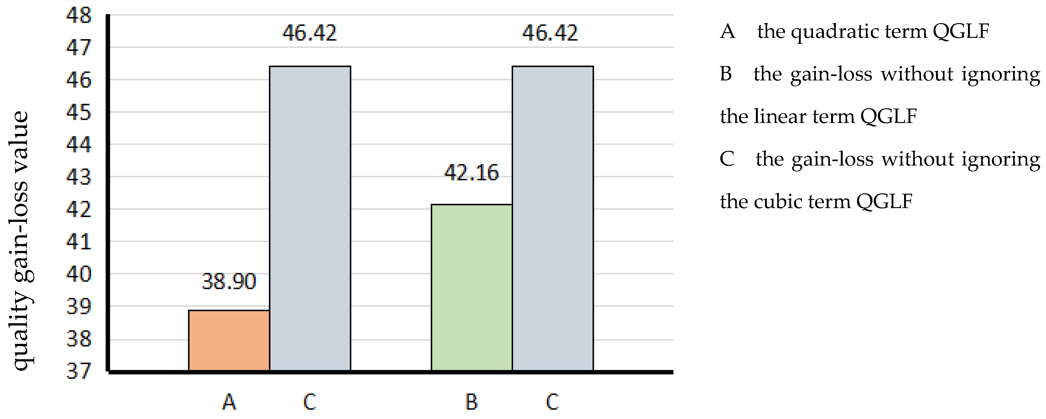
5.1. Case Analysis of the QGLF of the LBC

The specification limit of the continuous curing time for the concrete construction of a dam was ${\mathsf{\Delta }}_L=28d$, and the quality gain–loss was $A_L=60$ RMB/m³. The functional boundaries for continuous conservation time were presented as ${\mathsf{\Delta }}_{L0}=14d$, and the quality gain–loss was $A_{L0}=190$ RMB/m³. When ${\mathsf{\Delta }}_{L1}=32d$, $A_{L1}=48$ RMB/m³; the compensation was ${\sigma }_L=-10$ RMB/m³. There were ten randomly selected continuous curing times for concrete at this dam (unit: day): 40, 30, 34, 27, 35, 36, 32, 37, 33, and 29. The gain–loss value of concrete construction and maintenance was calculated by adopting the QGLF, QGLF considering primary term loss, and QGLF considering primary and cubic term losses.

(1) By substituting ${\mathsf{\Delta }}_L$, $A_L$, and ${\sigma }_L$ into the quadratic QGLF in Table 2 for calculation, the quadratic QGLF can be obtained using Equation (45):

$$L_{La}\left(y\right)=-10+\mathrm{54,880}\cdot {\displaystyle \frac{1}{y^2}}$$

(45)

(2) By substituting ${\mathsf{\Delta }}_L$, $A_L$, ${\mathsf{\Delta }}_{L0}$, $A_{L0}$, and ${\sigma }_L$ into the QGLF considering the primary term in Table 2 for calculation, QGLF considering primary term loss is shown in Equation (46):

$$L_{Lb}\left(y\right)=-10+560\cdot {\displaystyle \frac{1}{y}}+\mathrm{39,200}\cdot {\displaystyle \frac{1}{y^2}}$$

(46)

(3) By substituting ${\mathsf{\Delta }}_L$, $A_L$, ${\mathsf{\Delta }}_{L0}$, $A_{L0}$, ${\mathsf{\Delta }}_{L1}$, $A_{L1}$, and ${\sigma }_L$ into the QGLF considering the primary term in Table 2 for calculation, the QGLF considering primary and cubic term losses is shown in Equation (47):

$$L_L\left(y\right)=-10+1134\cdot {\displaystyle \frac{1}{y}}+\mathrm{22,923}\cdot {\displaystyle \frac{1}{y^2}}+\mathrm{55,750}\cdot {\displaystyle \frac{1}{y^3}}$$

(47)

Randomly selected conservation times were substituted into Equations (45)–(47), and the average quality gain–loss values were calculated: $\overline{L_{La}}=38.9$ RMB/m³, $\overline{L_{Lb}}=42.15$ RMB/m³, and $\overline{L_{Lc}}=46.42$ RMB/m³.

As can be seen from the above example, the value of the gain–loss without ignoring the cubic term quality gain–loss was 3.25 RMB/m³ more than the gain–loss value of the quadratic term QGLF; the value of the gain–loss without ignoring the cubic term QGLF was 4.27 RMB/m³ more than the value of the gain–loss without ignoring the linear term QGLF. The percentage discrepancy value between the estimated and actual losses was 9.19% (see Figure 7).

5.2. Case Analysis of QGLF of the SBC

The design target value for the concrete mix outlet temperature was 7 °C, the specification limit greater than the design target value $y$ was ${\mathsf{\Delta }}_S=3$ ℃, and the quality gain–loss was $A_S=65$ RMB/m³. The functional boundary of the product quality characteristics was ${\mathsf{\Delta }}_{S0}=5$ °C, and the quality gain–loss was $A_{S0}=155$ RMB/m³. When ${\mathsf{\Delta }}_{S1}=2$ °C, $A_{S1}=35$ RMB/m³; the compensation was ${\sigma }_S=-3$ RMB/m³. To assess the quality of dam concrete production, the differences between the outlet temperature and target value for 10 randomly selected concrete mixes (unit: day) were obtained: 0.2, 0.3, 0.5, 1.1, 1.2, 1.8, 1.5, 1.0, 0.8, and 0.4. The gain–loss value of concrete placement was calculated by adopting the quadratic QGLF, the QGLF considering primary term loss, and the QGLF considering primary and cubic term losses.

(1) The variables ${\mathsf{\Delta }}_S$, $A_S$, and ${\sigma }_S$ were substituted into the quadratic QGLF in Table 2 for calculation, and the quadratic QGLF was calculated using Equation (48):

$$L_{Sa}\left(y\right)=-3+4.8y^2$$

(48)

(2) The variables ${\mathsf{\Delta }}_S$, $A_S$, ${\mathsf{\Delta }}_{S0}$, $A_{S0}$, and ${\sigma }_S$ were substituted into the QGLF considering the primary term in Table 2 for calculation, and the QGLF considering the primary term loss was calculated using Equation (49):

$$L_{Sb}\left(y\right)=-3+10.333y+4.333y^2$$

(49)

(3) The variables ${\mathsf{\Delta }}_S$, $A_S$, ${\mathsf{\Delta }}_{S0}$, $A_{S0}$, ${\mathsf{\Delta }}_{S1}$, $A_{S1}$, and ${\sigma }_S$ were substituted into the QGLF considering the primary term in Table 2 for the calculation, and the QGLF considering the primary and cubic term losses was calculated using Equation (50):

$$L_{Sc}\left(y\right)=-3+15.333y+1.667y^2+0.333y^3$$

(50)

The randomly selected differences were substituted into each of the equations from Equations (48)–(50), and the average quality gain–loss values were calculated: $\overline{L_{Sa}}=1.954$ RMB/m³, $\overline{L_{Sb}}=10.565$ RMB/m³, and $\overline{L_{Sc}}=12.679$ RMB/m³.

As can be seen from the above example, the value of the gain–loss without ignoring the cubic term QGLF was 10.725 RMB/m³ more than the gain–loss value of the quadratic term QGLF; the value of the gain–loss without ignoring the cubic term QGLF was 2.114 RMB/m³ more than the value of the gain–loss without ignoring the linear term QGLF. The percentage discrepancy value between the estimated and actual losses was 20.00% (see Figure 8).

6. Conclusions

Based on the relationship graphs of the linear term, the quadratic term, and the cubic term quality loss functions in the QGLF of the LBC and the SBC, the intervals of the LBC and the SBC were designed when the cubic term losses were considered. The ratio of the quadratic term loss to the cubic term loss was used as a threshold, and a model for the LBC and the SBC of the QGLF was proposed when the tertiary term loss was considered. The formulas for calculating the loss coefficients of the first, second, and third terms in the lookahead and lookahead characteristic mass loss functions when considering the loss of the third term were solved. By calculating the quality gain–loss of the continuous curing time for dam concrete construction and the temperature of concrete pouring out of the machine, it was proved that the gain–loss value of QGLF without ignoring the cubic term was larger than that of QGLF without ignoring the linear term or only the quadratic term, which verifies the results of the research in this paper.

References

1. Genichi, T. Introduction to Quality Engineering; China Translation & Publishing Corporation: Beijing, China, 1985. [Google Scholar]
2. Cao, Y.L.; Yang, J.X.; Wu, Z.T.; Wu, L.Q. Robust tolerance design based on fuzzy quality loss. J. Zhejiang Univ. (Eng. Sci.) 2004, 38, 2–5. [Google Scholar] [CrossRef]
3. Zhao, Y.M.; Liu, D.S.; Zhang, J.; Liu, Q. Quality loss cost model and its application to products with multi-quality characteristics. J. Cent. South Univ. (Sci. Technol.) 2012, 43, 1753–1763. [Google Scholar]
4. Artiles-León, N. A pragmatic approach to multi-response problems using loss functions. Qual. Eng. 1996, 9, 213–220. [Google Scholar] [CrossRef]
5. Wang, J.P.; Tao, H.; Li, J.J. A multiple-parameter quality loss model. J. Northwest. Polytech. Univ. 2001, 19, 390–393. [Google Scholar]
6. Chang, Y.C.; Hung, W.L. LINEX loss functions with applications to determining the optimum process parameters. Qual. Quant. 2007, 41, 291–301. [Google Scholar] [CrossRef]
7. Deng, F.M. Analysis of quality loss in the autocorrelated process based on the quality loss function. Soft Sci. 2012, 26, 34–38. [Google Scholar]
8. Ding, L.P.; Jiang, L.P.; Chen, W.L. Robust selective assembly method for module instances based on quality loss function. J. Nanjing Univ. Aeronaut. Astronaut. 2012, 44, 543–547. [Google Scholar]
9. Duan, S.S.; Fan, S.H.; Huang, T.H.; Dong, L.J.; Fang, Y.X. The research of incremental model based on multivariate quality loss function. Mach. Des. Manuf. 2013, 51, 253–256. [Google Scholar]
10. Xue, L. Economic design of EWMA control charts with variable sampling intervals under preventive maintenance and quality loss functions. Oper. Res. Manag. Sci. 2020, 29, 116–121. [Google Scholar]
11. Zhang, L.; Dong, X.Y.; Li, X. Economic design of ARMA control charts based on the quality loss function. Stat. Decis. 2017, 7, 79–82. [Google Scholar]
12. Li, Y.P.; Liu, S.F.; Fang, Z.G.; Chen, H.Z. Parameter choice for multi quality-characteristics product based on stochastic grey target model. Ind. Eng. Manag. 2017, 22, 49–61. [Google Scholar]
13. Mao, K.; Liu, X.T.; Li, S.S.; Wang, X.X. Reliability analysis for mechanical parts considering hidden cost via the modified quality loss model. Qual. Reliab. Eng. Int. 2021, 37, 1373–1395. [Google Scholar] [CrossRef]
14. Zhang, Y.Y.; Song, M.S.; Han, Z.J. Designing of the quality loss function of the larger the better characteristic under not neglecting the linear term. J. Appl. Stat. Manag. 2013, 32, 486–491. [Google Scholar]
15. Zhang, Y.Y.; Song, M.S.; Han, Z.J.; Chen, X.L. Design of quality loss function under the smaller the better characteristic without neglecting the linear term. Ind. Eng. J. 2011, 14, 81–83. [Google Scholar]
16. Zhang, Y.Y.; Song, M.S.; Han, Z.J. Research on dynamic characteristic quality loss functions. China Qual. 2010, 92–94. [Google Scholar] [CrossRef]
17. Feng, Z.B.; Wang, J.J.; Ma, Y.Z. Bayesian modeling and robust parameter design based on multivariate Gaussian process model. Syst. Eng. Theory Pract. 2020, 40, 703–713. [Google Scholar]
18. Li, S.S.; Liu, X.T.; Wang, Y.S.; Wang, X.L. A cubic quality loss function and its applications. Qual. Reliab. Eng. Int. 2019, 35, 1161–1179. [Google Scholar] [CrossRef]
19. Li, S.S.; Liu, X.T.; Wang, Y.S.; Wang, X.L. Hidden quality cost function of a product based on the cubic approximation of the Taylor expansion. Int. J. Prod. Res. 2018, 56, 4762–4780. [Google Scholar] [CrossRef]
20. Zhang, B.; Han, Z.J.; Tang, Y. Optimal process mean and quality investment decisions based on the quality loss function. Stat. Decis. 2008, 18, 33–34. [Google Scholar]
21. Zhang, B.; Han, Z.J.; Cao, C.Z. Determination of the optimal process mean and the length of the production run. Appl. Stat. Manag. 2008, 27, 881–885. [Google Scholar]
22. Jin, Q. Optimizing the process mean of triangular distribution under quadratic asymmetric quality loss. J. Tianjin Univ. Sci. Technol. 2013, 28, 56–59. [Google Scholar]
23. Zhao, Y.M.; Liu, D.S.; Wen, Z.J. Optimal tolerance design of product based on service quality loss. Int. J. Adv. Manuf. Technol. 2016, 82, 1715–1724. [Google Scholar] [CrossRef]
24. Zhai, C.H.; Wang, J.J.; Feng, Z.B. Robust parameter design of multiple responses based on Gaussian process model. Syst. Eng. Electron. 2021, 43, 3683–3693. [Google Scholar]
25. Hu, T.; Yang, G.S. Tolerance optimization of construction quality factors considering capital constraints: A case study of PC component construction for viaducts. J. Eng. Manag. 2023, 37, 135–140. [Google Scholar]
26. Wu, J.J.; Zhou, M.; Cai, W. Parameter and tolerance concurrent design method considering process capability index. Mech. Sci. Technol. 2024, 43, 1747–1753. [Google Scholar]
27. Wu, J.J.; Cai, W.; Wan, F.X. Multi-objective robust optimization design of flexible hinges based on Taguchi method and cross-efficiency. Mach. Des. Manuf. 2024, 1140. [Google Scholar] [CrossRef]
28. Wang, B.; Li, Z.Y.; Gao, J.Y.; Heap, V. Critical quality source diagnosis for dam concrete construction based on quality gain-loss function. J. Eng. Sci. Technol. Rev. 2014, 7, 137–151. [Google Scholar] [CrossRef]
29. Wang, B.; Li, Q.K.; Yang, Q.; Liu, J.L.; Nie, X.T. Improvement of quadratic exponential quality gain–loss function and optimization of engineering specifications. Processes 2023, 11, 2225. [Google Scholar] [CrossRef]
30. Nie, X.; Liu, C.; Wang, B. Inverted normal quality gain-loss function and its application in water project construction. J. Coast. Res. 2020, 104, 415–420. [Google Scholar] [CrossRef]
31. Wang, B.; Fan, T.Y.; Tian, J.; Liu, M.Q.; Nie, X.T. Design of quality gain-loss function for larger-the-better characteristic and smaller-the-better characteristic under not neglecting the linear term loss and keeping compensation amount constant. Math. Pract. Theory 2019, 49, 153–160. [Google Scholar]
Figure 1. The loss relationship diagrams of the linear, quadratic, and cubic term losses in the QGLF for the LBC ( k L 1 k L 3 > k L 2 2 ).
Mathematics 13 00777 g001
Figure 2. The loss relationship diagrams of the linear, quadratic, and cubic term losses in the QGLF for the LBC ( k L 1 k L 3 k L 2 2 ).
Mathematics 13 00777 g002
Figure 3. Flow chart of the QGLF for LBC.
Mathematics 13 00777 g003
Figure 4. The loss relationship diagrams of the linear, quadratic, and cubic term losses in the QGLF for SBC ( k L 1 k L 3 > k L 2 2 ).
Mathematics 13 00777 g004
Figure 5. The loss relationship diagrams of the linear, quadratic, and cubic term losses in the QGLF for SBC ( k L 1 k L 3 k L 2 2 ).
Mathematics 13 00777 g005
Figure 6. Flow chart of the QGLF for SBC.
Mathematics 13 00777 g006
Figure 7. The comparison chart for the QGLF of the LBC.
Mathematics 13 00777 g007
Figure 8. The comparison chart for the QGLF of the SBC.
Mathematics 13 00777 g008