Stability-Optimized Graph Convolutional Network: A Novel Propagation Rule with Constraints Derived from ODEs

Abstract

The node representation learning capability of Graph Convolutional Networks (GCNs) is fundamentally constrained by dynamic instability during feature propagation, yet existing research lacks systematic theoretical analysis of stability control mechanisms. This paper proposes a Stability-Optimized Graph Convolutional Network (SO-GCN) that enhances training stability and feature expressiveness in shallow architectures through continuous–discrete dual-domain stability constraints. By constructing continuous dynamical equations for GCNs and rigorously proving conditional stability under arbitrary parameter dimensions using nonlinear operator theory, we establish theoretical foundations. A Precision Weight Parameter Mechanism is introduced to determine critical Frobenius norm thresholds through feature contraction rates, optimized via differentiable penalty terms. Simultaneously, a Dynamic Step-size Adjustment Mechanism regulates propagation steps based on spectral properties of instantaneous Jacobian matrices and forward Euler discretization. Experimental results demonstrate SO-GCN’s superiority: 1.1–10.7% accuracy improvement on homophilic graphs (Cora/CiteSeer) and 11.22–12.09% enhancement on heterophilic graphs (Texas/Chameleon) compared to conventional GCN. Hilbert–Schmidt Independence Criterion (HSIC) analysis reveals SO-GCN’s superior inter-layer feature independence maintenance across 2–7 layers. This study establishes a novel theoretical paradigm for graph network stability analysis, with practical implications for optimizing shallow architectures in real-world applications.

1. Introduction

Graph Convolutional Networks (GCNs) have emerged as a fundamental framework for graph data modeling by extending convolutional operations from Euclidean to non-Euclidean domains [1,2,3]. Since the seminal work of Kipf and Welling [4], GCNs have demonstrated remarkable success in social network analysis [5], recommendation systems [6], and biomolecular interaction prediction [7]. The core mechanism of GCNs—spectral-domain filtering for neighborhood information propagation—effectively captures topological features while maintaining computational efficiency. However, recent studies reveal that GCNs’ dynamic stability limitations in heterophilic graph structures constrain both theoretical interpretability and practical applicability [8,9].

1.1. Related Work

Despite significant advances in GCN performance [10,11,12,13], three fundamental theoretical gaps persist. First, a comprehensive framework for quantifying dynamic stability is lacking; while methods such as residual connections [14] and geometry-driven propagation [15] mitigate oversmoothing, rigorous mathematical characterization of Lyapunov stability remains absent. Although Chen et al. [16] demonstrated that an uncontrollable spectral radius causes deep GCN failure, stability mapping from parameter to feature space has not been established.

Second, discretization error control remains inadequate. Traditional forward Euler discretization often leads to numerical divergence in dynamic graph convolutions, and while Rusch et al. [17] introduced a gradient gating mechanism, fixed-step-size strategies still cause superlinear growth of node feature variance in heterophilic graphs, exacerbating training instability.

Third, existing studies predominantly address oversmoothing in deep networks, largely neglecting stability optimization in shallow architectures [18], resulting in suboptimal performance on complex graph structures.

1.2. Our Approach

To address these challenges, we propose the Stability-Optimized Graph Convolutional Network (SO-GCN), a dynamically stabilized framework that enhances intrinsic stability and feature representation in shallow architectures (2–7 layers). The innovations include the following:

• We developed a time-varying differential equation model for graph convolution propagation, establishing mathematical criteria for the Precision Weight Parameter Mechanism through stability mapping analysis.
• We formulated stability domain constraints for the weight matrix through Jacobian spectral analysis and proposed a Dynamic Step-size Adjustment Mechanism based on forward Euler discretization, applying stability mapping during gradient descent.
• We designed stable propagation rules integrating dual protection mechanisms with self-loop factors, optimizing feature stability and independence through quantitative metrics.

Recent theoretical advances, including adaptive frequency response filters [19,20,21] and potential connect of Lipschitz stability in graph neural diffusion  provide foundational support for our stability quantification framework  [22,23,24,25]. These developments not only validate our approach but also advance robust applications of GCNs in complex systems and depth optimization in shallow and stable networks.

2. Preliminaries

Based on Kipf’s seminal work [4], the standard Graph Convolutional Network (GCN) propagates node features by spectral filtering. The propagation rule is defined as follows:

$$H^{(l+1)}=\sigma \left({\tilde{D}}^{-{\displaystyle \frac{1}{2}}}\tilde{A}{\tilde{D}}^{-{\displaystyle \frac{1}{2}}}{H}^{\left(l\right)}{W}^{\left(l\right)}\right)$$

(1)

Consider an undirected graph $\mathcal{G}=(\mathcal{V},\mathcal{E})$, where $\mathcal{V}={\left\{v_i\right\}}_{i=1}^N$ denotes the node set and $\mathcal{E}\subseteq \mathcal{V}\times \mathcal{V}$ represents the edge set. The augmented adjacency matrix is $\tilde{A}=A+I_N\in {\mathbb{R}}^{N\times N}$, with A as the original adjacency matrix and $I_N$ as the identity matrix. Here, $H^{\left(l\right)}\in {\mathbb{R}}^{N\times d_l}$ is the feature matrix at layer l, $W^{\left(l\right)}\in {\mathbb{R}}^{d_l\times d_{l+1}}$ denotes the learnable weight matrix, and $\sigma (·)$ is the activation function. The initial input is $H^{\left(0\right)}=X\in {\mathbb{R}}^{N\times d_0}$, the node feature matrix.

Despite its effectiveness in graph modeling, this framework suffers from training instability and limited noise robustness on heterophilic graphs [8,9]. To address these limitations, we reformulate the graph convolution mechanism from a continuous dynamics perspective and establish a rigorous stability guarantee framework.

2.1. Continuous Dynamics Model

To establish the theoretical connection between graph convolutional networks and dynamical systems, we extend the discrete layer index l to a continuous time variable $t\in {\mathbb{R}}^{+}$, deriving the continuous propagation equation for graph convolution as follows:

$$\begin{array}{cc}\hfill {\displaystyle \frac{dH\left(t\right)}{dt}}& =\sigma \left(\mathcal{L}H\left(t\right)W\right),\mathcal{L}={\tilde{D}}^{-1/2}\tilde{A}{\tilde{D}}^{-1/2}\hfill \end{array}$$

(2)

where $H\left(t\right)\in {\mathbb{R}}^{N\times d_t}$ represents the node feature matrix at time t, $\mathcal{L}\in {\mathbb{R}}^{N\times N}$ denotes the symmetric normalized graph Laplacian operator, $W\left(t\right)\in {\mathbb{R}}^{d_t\times d_{t+1}}$ is the time-dependent parameter matrix, and $\sigma (·)$ indicates the element-wise activation function.

2.1.1. Stability Analysis of Equilibrium State

The existence of an equilibrium state is essential for stable propagation, as it enables the system to resist noise from minor disturbances or initial condition variations. Using fixed-point theory [26,27], we establish the following key result:

Theorem 1

(Existence of Equilibrium). The continuous propagation equation guarantees an equilibrium state when ${\parallel \mathcal{L}\parallel }_F,{\parallel W\parallel }_F<\infty$; the activation function σ is globally Lipschitz continuous. Then, there exists an equilibrium state $H^{\ast }\in {\mathbb{R}}^{N\times d_{t+1}}$ satisfying

$$\begin{array}{cc}\hfill H^{\ast }& =\sigma \left(\mathcal{L}{H}^{\ast }W\right)\hfill \end{array}$$

(3)

This differential equation characterizes the evolution dynamics of node features in continuous time. We analyze the system’s dynamic behavior near the equilibrium point $H^{\ast }$, where input and output feature dimensions are identical and Equation (3) holds. To quantify the system’s convergence rate, we define the feature contraction rate:

Definition 1

(Feature Contraction Rate). The instantaneous contraction rate of the propagation operator is

$$\begin{array}{cc}\hfill \gamma \left(t\right)& =\underset{H\ne 0}{sup}{\displaystyle \frac{{\parallel \mathcal{L}H\left(t\right)W\parallel }_F}{{\parallel H\left(t\right)\parallel }_F}}\hfill \end{array}$$

(4)

when $\gamma \left(t\right)\le 1$ and the system is asymptotically stable.

Based on this, we derive the theoretical foundation for the Precision Weight Parameter Mechanism (PW Mechanism):

Theorem 2

(Weight Frobenius Norm Constraint). When the weight matrix satisfies

$$\begin{array}{cc}\hfill {\parallel W\parallel }_F& \le {\displaystyle \frac{1}{\mathbb{E}\left[{\sigma }^{\prime }\right]·{\parallel \mathcal{L}\parallel }_F}}\hfill \end{array}$$

(5)

it ensures $\gamma \left(t\right)<1$, where $\mathbb{E}\left[{\sigma }^{\prime }\right]$ is the expected value of the activation function’s derivative.

2.1.2. Stability Guarantee of the Forward Euler Discretization Scheme

Discretizing Equation (2) by the forward Euler method yields the following:

$$\begin{array}{cc}\hfill H_{t+1}& =H_t+{\eta }_t\sigma \left(\mathcal{L}{H}_{t}W\right)\hfill \end{array}$$

(6)

where ${\eta }_t$ denotes the adaptive step size.

The stability of the discrete system depends on the spectral properties of the instantaneous Jacobian $J_t$, providing the theoretical foundation for the Dynamic Step-size Adjustment Mechanism (DS Mechanism):

Theorem 3

(Step Size Upper Bound Constraint). The discrete system achieves numerical stability when the step size upper bound ${\eta }_t$ satisfies

$$\begin{array}{cc}\hfill {\eta }_t& \le min\left({\displaystyle \frac{2}{|{\lambda }_{min}\left(J_t\right)|}},{\displaystyle \frac{1}{{\sigma }_{max}\left(J_t\right)}}\right)\hfill \end{array}$$

(7)

where $J_t=\mathcal{L}·\mathit{\text{diag}}\left({\sigma }^{\prime }\left(\mathcal{L}{H}_{t}W\right)\right)·W$ represents the instantaneous Jacobian matrix, ${\lambda }_{min}$ denotes the smallest eigenvalue modulus, and ${\sigma }_{max}$ signifies the largest singular value.

When the forward Euler discretization of the GCN continuous propagation Equation (Equation (6)) meets the stability condition (Equation (7)), we introduce a self-loop influence factor $\alpha \in [0,1]$ to enhance stability, yielding the discrete propagation equation:

$$H_{t+1}=\sigma \left(\left(I+{\eta }_t(\mathcal{L}-\alpha I)\right)H_{t}W\right)$$

(8)

We define $\widetilde{{\Omega }_t}=I+\eta (\mathcal{L}-\alpha I)$ as the discrete adjustment term, which balances node self-information preservation with neighborhood information aggregation. This formulation establishes a rigorous theoretical basis for SO-GCN’s stable propagation rule.

The proofs of Theorems 1–3 appear in Appendix A, Appendix B, and Appendix C, respectively.

3. Stability-Optimized Graph Convolutional Network

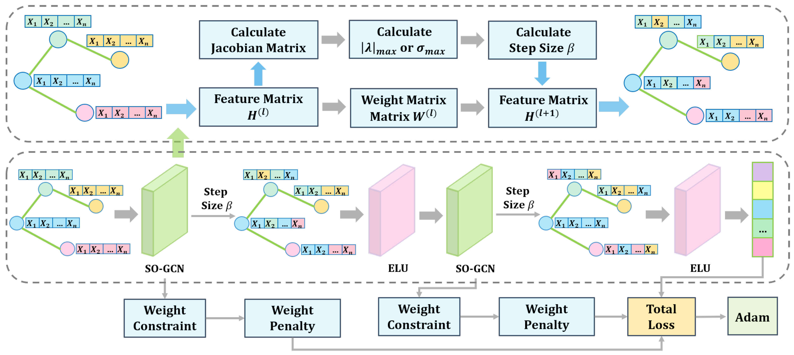
3.1. Network Overview

Based on the preceding theoretical results, we propose a stability propagation rule that integrates dynamic step-size adjustment, weight matrix norm constraints, and an upper-bound penalty term. By discretizing the propagation equation, we develop a Stability-Optimized Graph Convolutional Network (SO-GCN) with enhanced training stability, improved prediction accuracy, and superior loss convergence.The of SO-GCN with two layers is shown as Figure 1. During training, the network dynamically determines the weight matrix norm threshold to constrain parameter updates and optimizes parameter space distribution through a differentiable penalty term. Simultaneously, based on the spectral properties of the Jacobian matrix, we employ the forward Euler discretization method to dynamically adjust the step size and introduce a self-loop influence factor to enhance propagation stability.

This framework incorporates three modules into the GCN feature propagation process:

• Precision Weight Parameter Mechanism (PW Mechanism): constrains the Frobenius norm of the weight matrix through stability analysis of differential equations;
• Dynamic Step-size Adjustment Mechanism (DS Mechanism): adaptively controls the propagation step size based on the instantaneous Jacobian matrix;
• Stable propagation rule: combines the PW Mechanism and DS Mechanism to optimize both numerical stability and model expressiveness.

The basic framework of SO-GCN with two layers is as Figure 2.

3.2. Stability-Optimized Propagation Rule

To enhance graph filtering performance, we develop a stable propagation rule based on discrete dynamical system theory:

$$\begin{array}{c}\hfill H^{(l+1)}=\sigma \left(\left(I+{\eta }_l·(\mathcal{L}-\alpha I)\right)H^{\left(l\right)}{W}^{\left(l\right)}\right)\end{array}$$

(9)

where $\sigma (·)$ denotes the Leaky ReLU activation function, $\alpha \in [0,1]$ represents the self-loop influence factor, $W^{\left(l\right)}$ satisfies the norm constraint in the Precision Weight Parameter Mechanism, and ${\eta }_l$ is dynamically determined by the Dynamic Step-size Adjustment Mechanism. This rule maintains node self-information through the $\alpha I$ term while enabling adaptive neighborhood information aggregation via ${\tilde{\Omega }}_{\left(l\right)}$.

3.2.1. Precision Weight Parameter Mechanism

To accelerate optimization, we propose the Precision Weight Parameter Mechanism (PW Mechanism). The Frobenius norm threshold for the weight matrix at layer l is

$$\begin{array}{c}\hfill {\theta }^{\left(l\right)}={\left(\mathbb{E}\left[{\sigma }^{\prime }\right]{\parallel \mathcal{L}\parallel }_F\right)}^{-1}\end{array}$$

(10)

where $\mathbb{E}\left[{\sigma }^{\prime }\right]={\displaystyle \frac{1}{N{d}_l}}{\sum }_{i,j}{\sigma }^{\prime }\left(M_{ij}\right)$ is the expected value of the activation function derivative, $M^{\left(l\right)}=\mathcal{L}{H}^{\left(l\right)}{W}^{\left(l\right)}$ is the intermediate feature matrix, and $\mathcal{L}={\tilde{D}}^{-1/2}\tilde{A}{\tilde{D}}^{-1/2}$ is the symmetric normalized graph Laplacian.

First, the mechanism inputs node features $H^{\left(l\right)}$ into SO-GCN for standard graph convolution, computes the norm threshold for layer l, and performs two-stage optimization based on Theorem 2 to obtain network response distribution characteristics. When $\parallel W^{\left(l\right)}{\parallel }_F>{\theta }^{\left(l\right)}$, it applies Frobenius norm projection,

$$\begin{array}{c}\hfill {\widehat{W}}^{\left(l\right)}={\theta }^{\left(l\right)}·W^{\left(l\right)}/{\parallel W^{\left(l\right)}\parallel }_F\end{array}$$

(11)

to constrain parameters within the stability domain. Simultaneously, it constructs a quadratic gradient penalty term:

$$\begin{array}{c}\hfill \mathcal{P}=max{\left(0,\parallel W^{\left(l\right)}{\parallel }_F-{\theta }^{\left(l\right)}\right)}^2\end{array}$$

(12)

This penalty term guides parameter convergence through backpropagation, preventing it from exceeding the predefined range. The pseudocode for the Precision Weight Parameter Mechanism is as Algorithm 1:

Algorithm 1: Precision Weight Parameter Mechanism

1: Require: Feature matrix $H^{\left(l\right)}$, parameter matrix $W^{\left(l\right)}$, graph Laplacian $\mathcal{L}$ 2: Ensure: Stable parameter matrix ${\widehat{W}}^{\left(l\right)}$, penalty term $\mathcal{P}$ 3: $M^{\left(l\right)}\leftarrow \mathcal{L}{H}^{\left(l\right)}{W}^{\left(l\right)}$ 4: $\mathbb{E}\left[{\sigma }^{\prime }\right]\leftarrow {\displaystyle \frac{1}{N{d}_l}}{\sum }_{i,j}{\sigma }^{\prime }\left(M_{ij}\right)$                             ▹ Expectation of activation derivative 5: ${\theta }^{\left(l\right)}\leftarrow (\mathbb{E}\left[{\sigma }^{\prime }\right]{\parallel \mathcal{L}\parallel }_F{)}^{-1}$ 6: if$\parallel W^{\left(l\right)}{\parallel }_F > {\theta }^{\left(l\right) }$then 7:     ${\widehat{W}}^{\left(l\right)}\leftarrow {\theta }^{\left(l\right)}{W}^{\left(l\right)}/{\parallel W^{\left(l\right)}\parallel }_F$                                                       ▹ Parameter projection 8: else 9:     ${\widehat{W}}^{\left(l\right)}\leftarrow W^{\left(l\right)}$ 10: end if 11: $\mathcal{P}\leftarrow max(0, \parallel W^{\left(l\right)}{{\parallel }_F-{\theta }^{\left(l\right)})}^2$                                             ▹ Quadratic penalty term 12: return ${\widehat{W}}^{\left(l\right)},\mathcal{P}$

This strategy combines hard constraints with soft penalties to maintain numerical stability while preserving end-to-end differentiability, preventing extreme weight variations during iterations and ensuring smooth feature updates. After integrating the Precision Weight Parameter Mechanism into the baseline GCN, we refer to the resulting model as the Precision Weight Graph Convolutional Network (PW-GCN).

3.2.2. Dynamic Step-Size Adjustment Mechanism

To enhance inter-layer propagation stability, we propose the Dynamic Step-size Adjustment Mechanism (DS Mechanism). The instantaneous Jacobian matrix is defined as

$$\begin{array}{c}\hfill J^{\left(l\right)}=\mathcal{L}·\mathrm{diag}\left({\sigma }^{\prime }\left(M^{\left(l\right)}\right)\right)·W^{\left(l\right)},M^{\left(l\right)}=\mathcal{L}{H}^{\left(l\right)}{W}^{\left(l\right)}\end{array}$$

(13)

Based on Theorem 3’s analysis of $J^{\left(l\right)}$’s spectral properties, the upper bound of the step size is

$$\begin{array}{c}\hfill {\eta }_l\le min\left({\displaystyle \frac{2}{|{\lambda }_{min}\left(J^{\left(l\right)}\right)|}},{\displaystyle \frac{1}{{\sigma }_{max}\left(J^{\left(l\right)}\right)}}\right)\end{array}$$

(14)

where ${\lambda }_{min}$ denotes the smallest eigenvalue modulus and ${\sigma }_{max}$ represents the largest singular value.

Using the power iteration method to estimate the principal eigenvector, we set the step size as ${\eta }_l\leftarrow 0.85{\eta }_{max}$, where the safety factor of 0.85 compensates for spectral estimation errors and ensures numerical stability. This strategy maximizes information propagation efficiency while maintaining discrete system stability. The pseudocode for the Dynamic Step-size Adjustment Mechanism is as follows Algorithm 2.

Integrating the Dynamic Step-size Adjustment Mechanism into the baseline GCN yields the Dynamic Step Graph Convolutional Network (DS-GCN). The Precision Weight Parameter Mechanism ensures weight matrix stability through Frobenius norm projection and gradient penalties, while the Dynamic Step-size Adjustment Mechanism further optimizes discrete error accumulation via safety-factor-adjusted step sizes. The stable propagation rule, combining both mechanisms, provides theoretical support for enhancing feature output stability.

Algorithm 2: Dynamic Step-size Adjustment Mechanism

1: Require: Feature matrix $H^{\left(l\right)}$, parameter matrix $W^{\left(l\right)}$, graph Laplacian $\mathcal{L}$ 2: Ensure: Stable step size ${\eta }_l$, propagation matrix $H^{(l+1)}$ 3: $J^{\left(l\right)}\leftarrow \mathcal{L}·\mathrm{diag}\left({\sigma }^{\prime }\left(M^{\left(l\right)}\right)\right)·W^{\left(l\right)}$                                             ▹$M^{\left(l\right)}=\mathcal{L}{H}^{\left(l\right)}{W}^{\left(l\right)}$ 4: $v\leftarrow \mathrm{random}\mathrm{unit}\mathrm{vector}\mathrm{in}{\mathbb{R}}^N$ 5: for $k=1$ to K do 6:     $v_k\leftarrow J^{\left(l\right)}{v}_k$ 7:     $v_{k+1}\leftarrow v_k/{\parallel v_k\parallel }_2$ 8: end for 9: $\widehat{\sigma }\leftarrow {\parallel J^{\left(l\right)}v\parallel }_2$                                                            ▹ Spectral norm estimation 10: ${\eta }_{max}\leftarrow min\left({\displaystyle \frac{2}{|{\lambda }_{min}\left(J^{\left(l\right)}\right)|}},{\displaystyle \frac{1}{\widehat{\sigma }}}\right)$ 11: ${\eta }_l\leftarrow 0.85{\eta }_{max}$                                                                            ▹ Safety factor 12: $H^{(l+1)}\leftarrow \sigma \left(\left(I+{\eta }_l·(\mathcal{L}-\alpha I)\right)H^{\left(l\right)}{W}^{\left(l\right)}\right)$ 13: return  ${\eta }_l,H^{(l+1)}$

4. Experiments

This study conducts systematic validation on three homophilic graph datasets (Cora, CiteSeer, and PubMed) [20] and three heterophilic graph datasets (Chameleon, Texas, and Squirrel) [5]. We perform comprehensive ablation studies with four architectures: GCN, PW-GCN, DS-GCN, and SO-GCN. Model performance is evaluated through semi-supervised node classification tasks and compared to the performance of mainstream methods including GIN, GraphSAGE, GAT, and GCN. Our experimental setup adopts a learning rate of 0.01, 64-dimensional embeddings, a dropout rate of 0.5, and an $\alpha$ parameter of 0.5.

Table 1. Dataset statistics.

Dataset	Nodes	Edges	Classes	Features	Homophily Level
Cora	2708	5429	7	1433	0.81
CiteSeer	3327	4732	6	3703	0.74
PubMed	19,717	44,338	3	500	0.80
Chameleon	2277	36,101	3	2325	0.18
Texas	183	309	5	1703	0.11
Squirrel	5201	217,073	3	2089	0.018

summarizes the topological statistics of the datasets, where homophily metrics quantitatively verify structural heterogeneity.

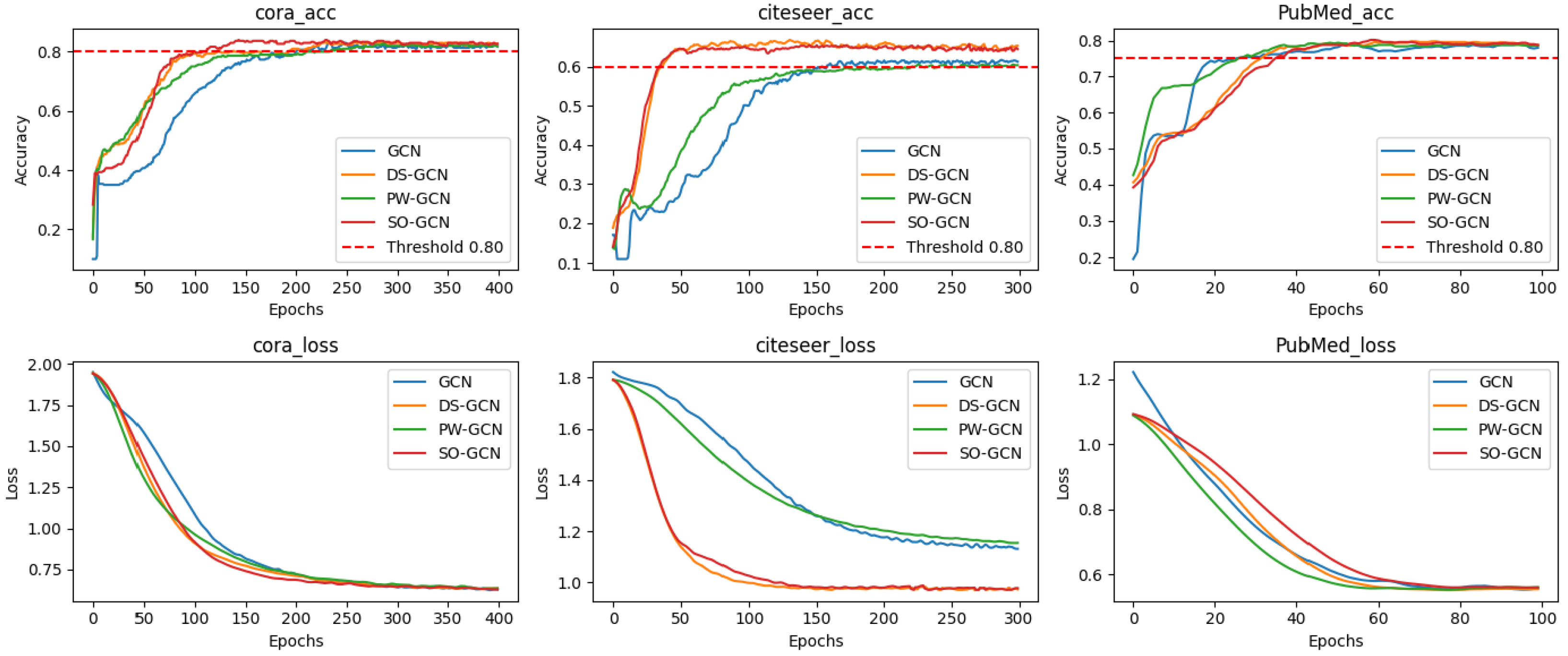
4.1. Experiment Results and Analysis

Table 2. Mean accuracy (%) of SO-GCN in two-layer ablation experiment.

Method	Cora	CiteSeer	PubMed	Texas	Chameleon	Squirrel	Avg
GCN	83.60	50.23	75.70	44.74	46.55	68.08	61.48
PW-GCN	84.50	50.53	77.53	50.36	46.20	67.13	62.71
DS-GCN	84.20	58.07	76.07	51.30	52.25	70.18	65.34
SO-GCN	84.70	60.90	78.40	56.8	57.77	71.07	68.01

presents a classification accuracy comparison for GCN, PW-GCN, DS-GCN, and SO-GCN across six benchmark datasets. The results demonstrate significant synergistic optimization effects between the Precision Weight Parameter Mechanism and the Dynamic Step-size Adjustment Mechanism in SO-GCN.

On homophilic datasets such as Cora and PubMed, PW-GCN improves accuracy by 0.9–1.8% through the Precision Weight Parameter Mechanism’s optimization of information propagation efficiency. However, its accuracy decreases by 0.35% on heterophilic graphs such as Chameleon, suggesting that using this mechanism alone can amplify noise. In contrast, DS-GCN achieves performance gains of 6.56% and 5.7% on Texas and Chameleon, respectively, through the Dynamic Step-size Adjustment Mechanism, effectively suppressing noise propagation in heterophilic graphs. The combined model SO-GCN achieves an average 11.65% improvement in accuracy on heterophilic datasets, demonstrating the complementary nature of the dual stabilization mechanisms.

Figure 3 further reveals the dynamic properties of the four models’ training: SO-GCN’s loss curve fluctuates significantly less than GCN’s, confirming the improvement in training stability due to the Dynamic Step-size Adjustment Mechanism. On PubMed’s sparse graph, PW-GCN converges the fastest, but its overall performance is best, with faster convergence, lower training loss (on average), and smoother accuracy curves.

This paper validates the effectiveness of SO-GCN through semi-supervised node classification tasks across six benchmark datasets. As shown in

Table 3. Mean accuracy (%) comparison across six benchmark networks with two layers.

Method	Cora	CiteSeer	PubMed	Texas	Chameleon	Squirrel
MLP	57.00	53.35	72.90	67.18	51.44	38.56
ChebNet	73.60	53.85	69.00	73.78	55.77	39.75
GIN	64.20	44.80	73.30	59.46	68.64	42.75
GraphSAGE	78.00	52.19	76.00	56.76	65.67	53.20
GCN	83.60	50.23	75.70	44.74	46.55	68.08
GAT	84.10	48.57	77.70	46.85	57.31	43.65
SO-GCN	84.70	60.90	78.40	56.83	57.77	71.07

, SO-GCN achieves an average classification accuracy of 68.01%, a 10.8% improvement over baseline GCN. Notably, on heterophilic graphs, the model achieves 56.83% and 71.07% accuracy on the Texas and Squirrel datasets, respectively, significantly outperforming models such as GAT.

This indicates that the stability propagation rule based on stability theory effectively optimizes information flow and enhances the network’s ability to capture graph signals.

4.2. Depth Analysis and Feature Preservation

To explore performance variations in shallow networks, we compare SO-GCN and GCN on classification accuracy across two- to seven-layer configurations on six benchmark datasets, as shown in

Table 4. Performance comparison across models with different layer configurations.

Dataset	Model	2 Layers	3 Layers	4 Layers	5 Layers	6 Layers	7 Layers
Cora	GCN	0.836	0.750	0.707	0.472	0.431	0.413
	SO-GCN	0.847	0.791	0.738	0.574	0.568	0.557
CiteSeer	GCN	0.502	0.413	0.302	0.273	0.277	0.274
	SO-GCN	0.609	0.519	0.460	0.381	0.374	0.369
PubMed	GCN	0.757	0.749	0.758	0.532	0.479	0.458
	SO-GCN	0.784	0.761	0.759	0.684	0.607	0.554

:

SO-GCN consistently outperforms GCN across all six benchmark datasets and layer configurations, particularly showing a 15.2% improvement in accuracy on the five-layer configuration of PubMed. This validates the framework’s ability to alleviate vanishing gradients by optimizing gradient stability and feature smoothness.

We quantify feature preservation through Hilbert–Schmidt Independence Criterion (HSIC) analysis between network layers. As shown in

Table 5. HSIC values across different datasets and models.

Dataset	Layers	Model	HSIC (Layers 1–2)	HSIC (Input–Layer 1)
Cora	2	GCN	0.18 ± 0.02	0.40 ± 0.03
		SO-GCN	0.10 ± 0.01	0.38 ± 0.02
	4	GCN	0.25 ± 0.03	0.32 ± 0.04
		SO-GCN	0.15 ± 0.02	0.35 ± 0.03
	7	GCN	0.29 ± 0.04	0.28 ± 0.05
		SO-GCN	0.18 ± 0.03	0.33 ± 0.04
CiteSeer	2	GCN	0.22 ± 0.03	0.35 ± 0.04
		SO-GCN	0.12 ± 0.02	0.34 ± 0.03
	4	GCN	0.31 ± 0.04	0.25 ± 0.05
		SO-GCN	0.20 ± 0.03	0.30 ± 0.04
	7	GCN	0.36 ± 0.05	0.21 ± 0.06
		SO-GCN	0.25 ± 0.04	0.28 ± 0.05
PubMed	2	GCN	0.15 ± 0.02	0.45 ± 0.03
		SO-GCN	0.08 ± 0.01	0.43 ± 0.02
	4	GCN	0.20 ± 0.03	0.38 ± 0.04
		SO-GCN	0.12 ± 0.02	0.40 ± 0.03
	7	GCN	0.26 ± 0.04	0.30 ± 0.05
		SO-GCN	0.20 ± 0.03	0.40 ± 0.03

, SO-GCN reduces inter-layer HSIC values by 16.7% in seven-layer PubMed configurations compared to GCN, demonstrating effective prevention of feature homogenization while preserving original graph structural information.

4.3. Computational Complexity Analysis

The above experimental results from multiple dimensions confirm that the SO-GCN framework, through the synergistic Precision Weight Parameter Mechanism and Dynamic Step-size Adjustment Mechanism, enhances model performance. However, its computational complexity inevitably increases in the following two aspects: (1) dynamic learning rate calculation and spectral analysis of density matrix squared neighborhoods introduce $O\left(N^2{d}_{out}\right)$ extra overhead; (2) the Precision Weight Parameter Mechanism requires calculating the Frobenius norm, resulting in an additional $O\left(N{d}_{in}{d}_{out}\right)$ cost, where $d_{in}$ and $d_{out}$ are the input and output feature dimensions. For large-scale graph data, Nyström low-rank approximation can be applied to reduce matrix computation complexity to $O\left(N{r}^2\right)(r\ll N)$, achieving a balance between efficiency and performance.

5. Conclusions

This study systematically validates the effectiveness of the SO-GCN model in semi-supervised node classification tasks. Experimental results demonstrate that the stability propagation rule, combining the Precision Weight Parameter Mechanism and the Dynamic Step-size Adjustment Mechanism, significantly enhances model performance: on homophilic graphs such as Cora and CiteSeer, SO-GCN improves classification accuracy by 1.1–10.7% compared to traditional GCN; on heterophilic graphs such as Texas and Chameleon, accuracy increases by 11.22–12.09% over the baseline model through dynamic adjustment of neighborhood information aggregation intensity. HSIC analysis further reveals that SO-GCN reduces inter-layer feature homogenization by 16.7% compared to GCN, effectively mitigating the gradient vanishing problem in shallow networks through optimized gradient propagation stability.

From an application perspective, SO-GCN’s architectural characteristics provide significant advantages in the following scenarios:

• In heterophilic graph settings such as social network anomaly detection, the Dynamic Step-size Adjustment Mechanism dynamically suppresses noise propagation through spectral characteristic perception;
• On knowledge graphs with sparse features but complex structures, such as biomedical networks, the Precision Weight Parameter Mechanism optimizes information propagation efficiency through Frobenius norm constraints;
• In industrial-grade graph computing systems (e.g., multi-hop inference in recommendation systems), the synergistic effect of dual stabilization mechanisms ensures numerical stability during higher-order propagation.

References

1. Bruna, J.; Zaremba, W.; Szlam, A.; LeCun, Y. Spectral networks and locally connected networks on graphs. In Proceedings of the International Conference on Learning Representations (ICLR), Banff, AB, Canada, 14–16 April 2014. [Google Scholar]
2. Shuman, D.I.; Narang, S.K.; Frossard, P.; Ortega, A.; Vandergheynst, P. The emerging field of signal processing on graphs: Extending high-dimensional data analysis to networks and other irregular domains. IEEE Signal Process. Mag. 2013, 30, 83–98. [Google Scholar] [CrossRef]
3. Defferrard, M.; Bresson, X.; Vandergheynst, P. Convolutional neural networks on graphs with localized spectral filtering. In Proceedings of the Advances in Neural Information Processing Systems, Barcelona, Spain, 5–10 December 2016; pp. 3844–3852. [Google Scholar]
4. Kipf, T.N.; Welling, M. Semi-supervised classification with graph convolutional networks. arXiv 2016, arXiv:1609.02907. [Google Scholar]
5. Hamilton, W.L.; Ying, R.; Leskovec, J. Inductive representation learning on large graphs. In Proceedings of the Advances in Neural Information Processing Systems, Long Beach, CA, USA, 4–9 December 2017; pp. 1024–1034. [Google Scholar]
6. Ying, R.; He, R.; Chen, K.; Eksombatchai, P.; Hamilton, W.L.; Leskovec, J. Graph convolutional neural networks for web-scale recommender systems. In Proceedings of the 24th ACM SIGKDD International Conference on Knowledge Discovery & Data Mining, London, UK, 19–23 August 2018; pp. 974–983. [Google Scholar]
7. Fout, A.; Byrd, J.; Shariat, B.; Ben-Hur, A. Protein interface prediction using graph convolutional networks. In Proceedings of the Advances in Neural Information Processing Systems, Long Beach, CA, USA, 4–9 December 2017; pp. 6533–6542. [Google Scholar]
8. Li, X.; Chen, S.; Hu, X.; Yang, J. Understanding the Disharmony between Dropout and Batch Normalization by Variance Shift. arXiv 2018, arXiv:1801.05134. [Google Scholar]
9. Oono, K.; Suzuki, T. Graph Neural Networks Exponentially Lose Expressive Power for Node Classification. arXiv 2019, arXiv:1905.10947. Available online: https://api.semanticscholar.org/CorpusID:209994765 (accessed on 27 May 2019).
10. Wang, X.; Zhang, M. How Powerful are Spectral Graph Neural Networks. In Proceedings of the 39th International Conference on Machine Learning, PMLR, Baltimore, MD, USA, 17–23 July 2022; pp. 23341–23362. [Google Scholar]
11. Chien, E.; Peng, J.; Li, P.; Milenkovic, O. Adaptive Universal Generalized PageRank Graph Neural Network. arXiv 2020, arXiv:2001.06922. [Google Scholar]
12. Zhou, J.; Cui, G.; Hu, S.; Zhang, Z.; Yang, C.; Liu, Z.; Wang, L.; Li, C.; Sun, M. Graph neural networks: A review of methods and applications. AI Open 2020, 1, 57–81. [Google Scholar] [CrossRef]
13. Xu, B.; Shen, H.; Cao, Q.; Cen, K.; Cheng, X. Graph convolutional networks using heat kernel for semi-supervised learning. In Proceedings of the 28th International Joint Conference on Artificial Intelligence, Macao, China, 10–16 August 2019; pp. 1928–1934. [Google Scholar]
14. Li, Q.; Han, Z.; Wu, X.-M. Deeper insights into graph convolutional networks for semi-supervised learning. In Proceedings of the Thirty-Second AAAI Conference on Artificial Intelligence, New Orleans, LA, USA, 2–7 February 2018; pp. 3538–3545. [Google Scholar]
15. Pei, H.; Wei, B.; Chang, K.C.-C.; Lei, Y.; Yang, B. Geom-GCN: Geometric Graph Convolutional Networks. arXiv 2020, arXiv:2002.05287. [Google Scholar]
16. Chen, D.; Liao, R. Stability and Generalization of Graph Neural Networks via Spectral Dynamics. In Proceedings of the 38th International Conference on Machine Learning, Virtual, 18–24 July 2021; pp. 11289–11302. [Google Scholar]
17. Rusch, T.K.; Bronstein, M.; Mishra, S. Gradient Gating for Deep Multi-Rate Learning on Graphs. In Advances in Neural Information Processing Systems; The MIT Press: Cambridge, MA, USA, 2022; pp. 22136–22149. [Google Scholar]
18. Topping, J.; Giovanni, F.D.; Chamberlain, B.P.; Dong, X.; Bronstein, M.M. Understanding Over-Squashing and Bottlenecks on Graphs via Curvature. In Proceedings of the 10th International Conference on Learning Representations, Virtual, 25–29 April 2022. [Google Scholar]
19. Dong, Y.; Ding, K.; Jalaeian, B.; Ji, S.; Li, J. AdaGNN: Graph Neural Networks with Adaptive Frequency Response Filter. In Proceedings of the 30th ACM International Conference on Information & Knowledge Management, Virtual Event, Australia, 1–5 November 2021. [Google Scholar]
20. Yang, Z.; Cohen, W.; Salakhutdinov, R. Revisiting semi-supervised learning with graph embeddings. In Proceedings of the International Conference on Machine Learning (ICML), New York, NY, USA, 19–24 June 2016. [Google Scholar]
21. Lim, D.; Robinson, J.; Zhao, L.; Smidt, T.; Sra, S.; Maron, H.; Jegelka, S. Sign and basis invariant networks for spectral graph representation learning. In Proceedings of the International Conference on Learning Representations (ICLR), Virtual, 1 May 2023. [Google Scholar]
22. Metz, L.; Maheswaranathan, N.; Freeman, C.D.; Poole, B.; Sohl-Dickstein, J.N. Tasks, stability, architecture, and compute: Training more effective learned optimizers, and using them to train themselves. arXiv 2009, arXiv:2009.11243. [Google Scholar]
23. Haber, E.; Lensink, K.; Treister, E.; Ruthotto, L. IMEXnet: A Forward Stable Deep Neural Network. In Proceedings of the 36th International Conference on Machine Learning, Long Beach, CA, USA, 9–15 June 2019; pp. 2525–2534. [Google Scholar]
24. Haber, E.; Ruthotto, L. Stable architectures for deep neural networks. Inverse Probl. 2018, 34, 014004. [Google Scholar] [CrossRef]
25. Haber, E.; Ruthotto, L.; Holtham, E. Learning across scales—A multiscale method for convolution neural networks. arXiv 2017, arXiv:1703.02009. [Google Scholar] [CrossRef]
26. Brouwer, L.E.J. Über Abbildung von Mannigfaltigkeiten. Math. Ann. 1911, 71, 97–115. [Google Scholar] [CrossRef]
27. Banach, S. Sur les opérations dans les ensembles abstraits et leur application aux équations intégrales. Fundam. Math. 1922, 3, 133–181. [Google Scholar] [CrossRef]
Figure 1. Workflow of stability-Optimized Graph Convolutional Network with Two layers.
Mathematics 13 00761 g001
Figure 2. Basic framework of Stability-Optimized Graph Convolutional Network with Two Layers.
Mathematics 13 00761 g002
Figure 3. Training process of four networks with two layers on homophilic graph datasets.
Mathematics 13 00761 g003