

A Time–Space Numerical Procedure for Solving the Sideways Heat Conduction Problem

Abstract
1. Introduction
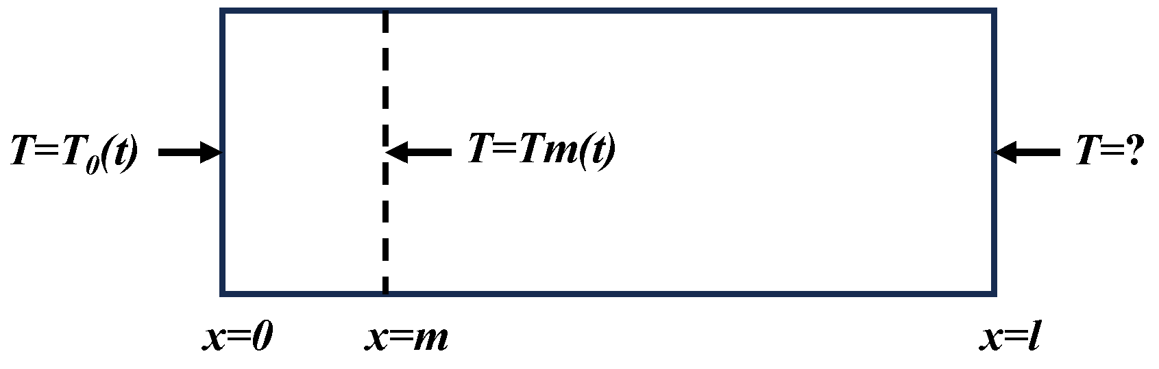
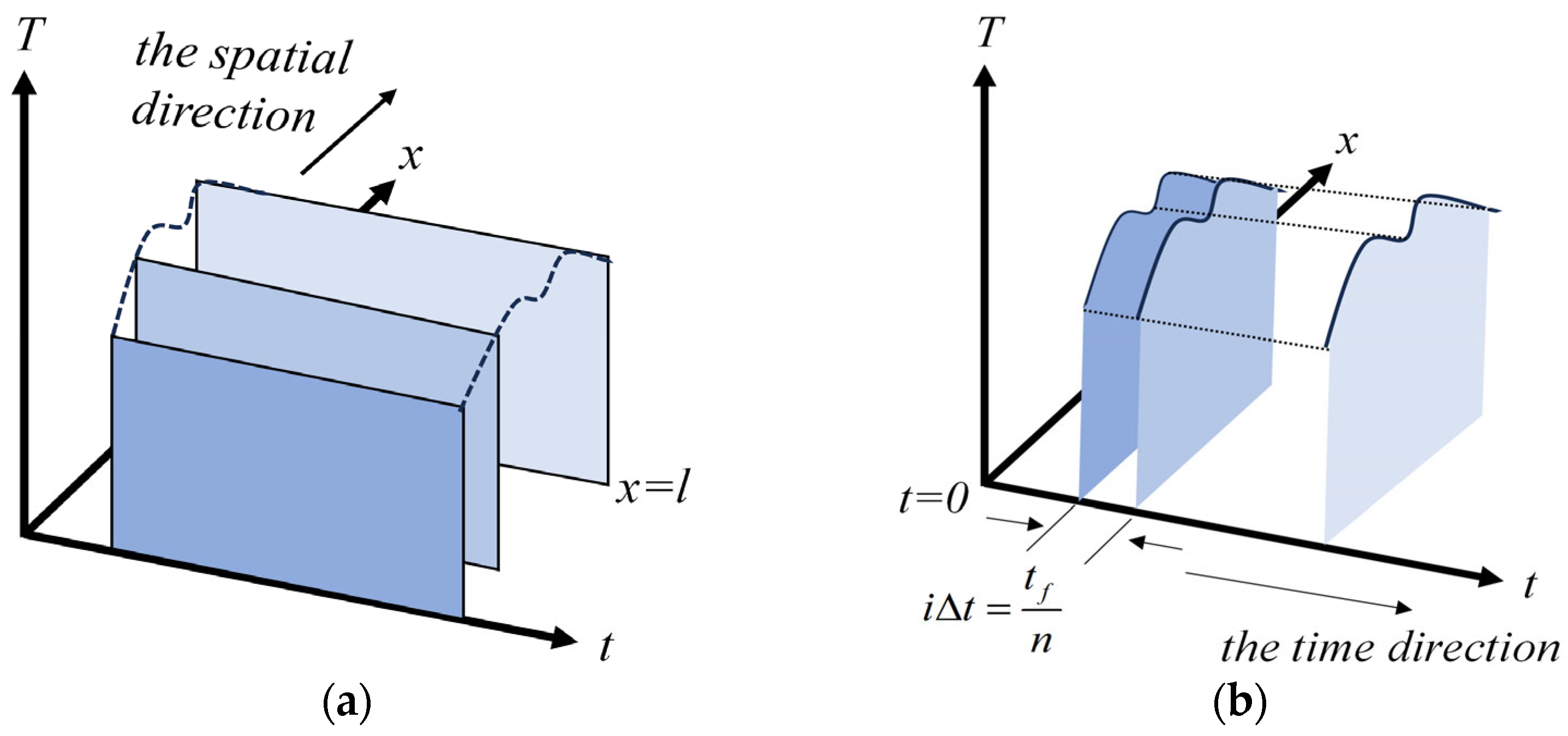
2. Governing Equation
3. The Numerical Procedures
4. Mathematical Backgrounds
4.1. The GPS
4.2. One-Step Lie Group Transformation
4.3. The Lie Group Shooting Equation
4.4. To Estimate by a Backward-in-Time Explicit Procedure
5. Numerical Examples
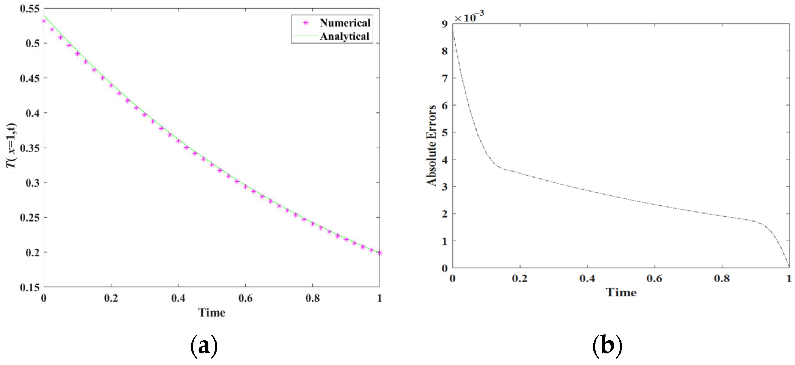
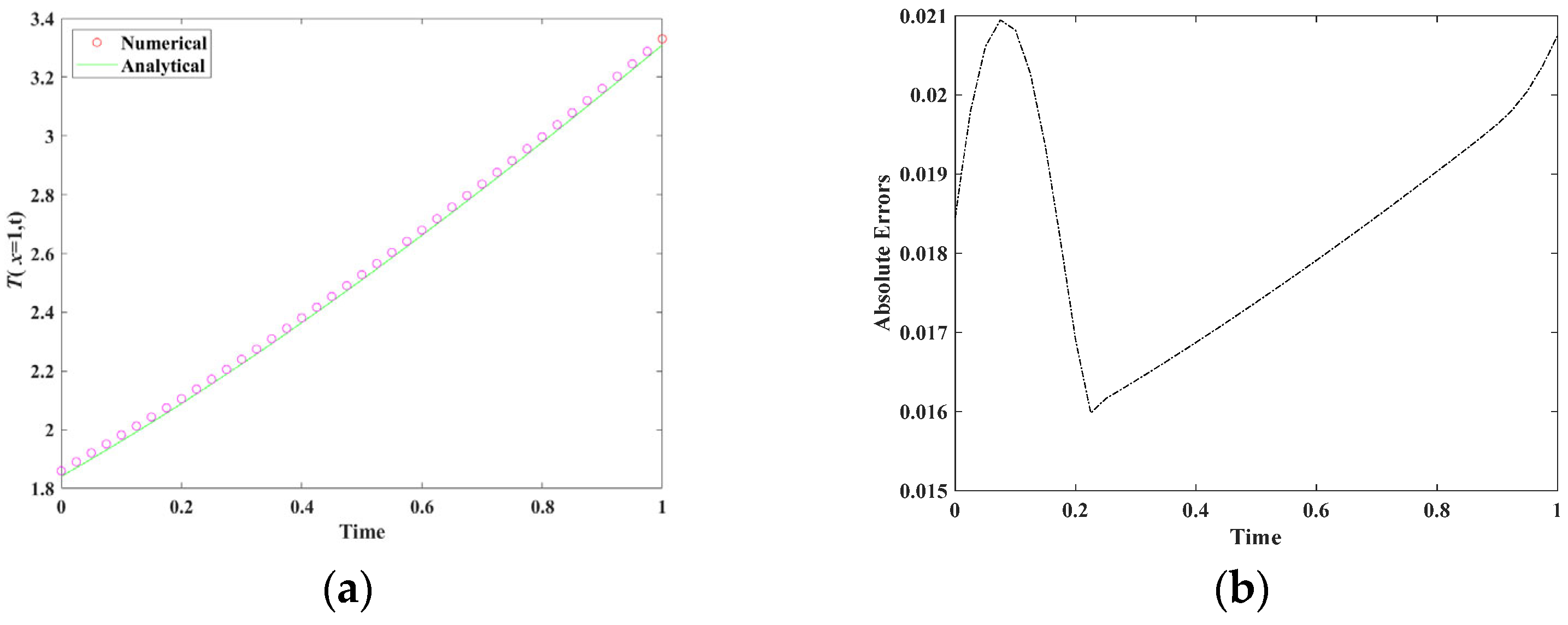
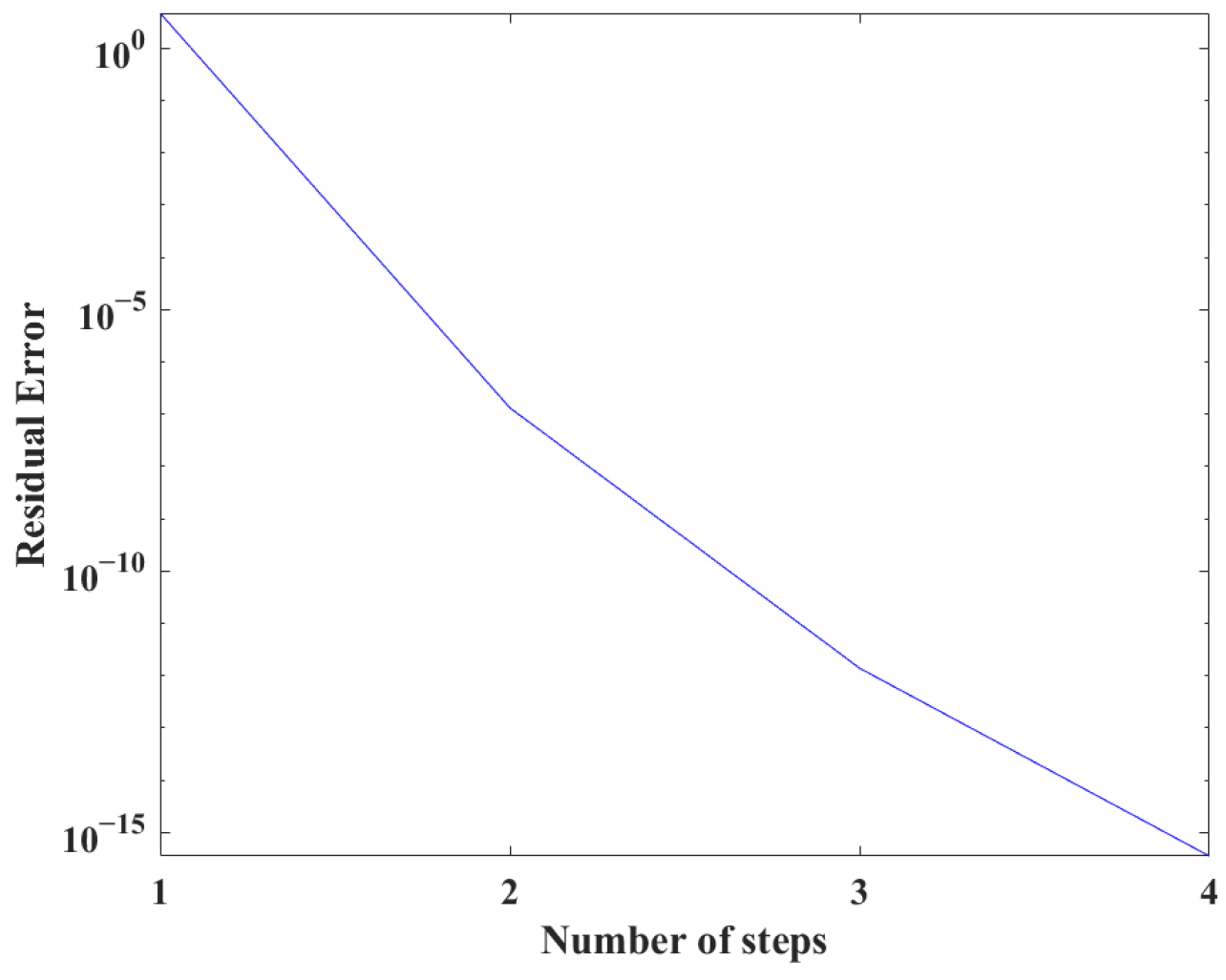
5.1. Example 1
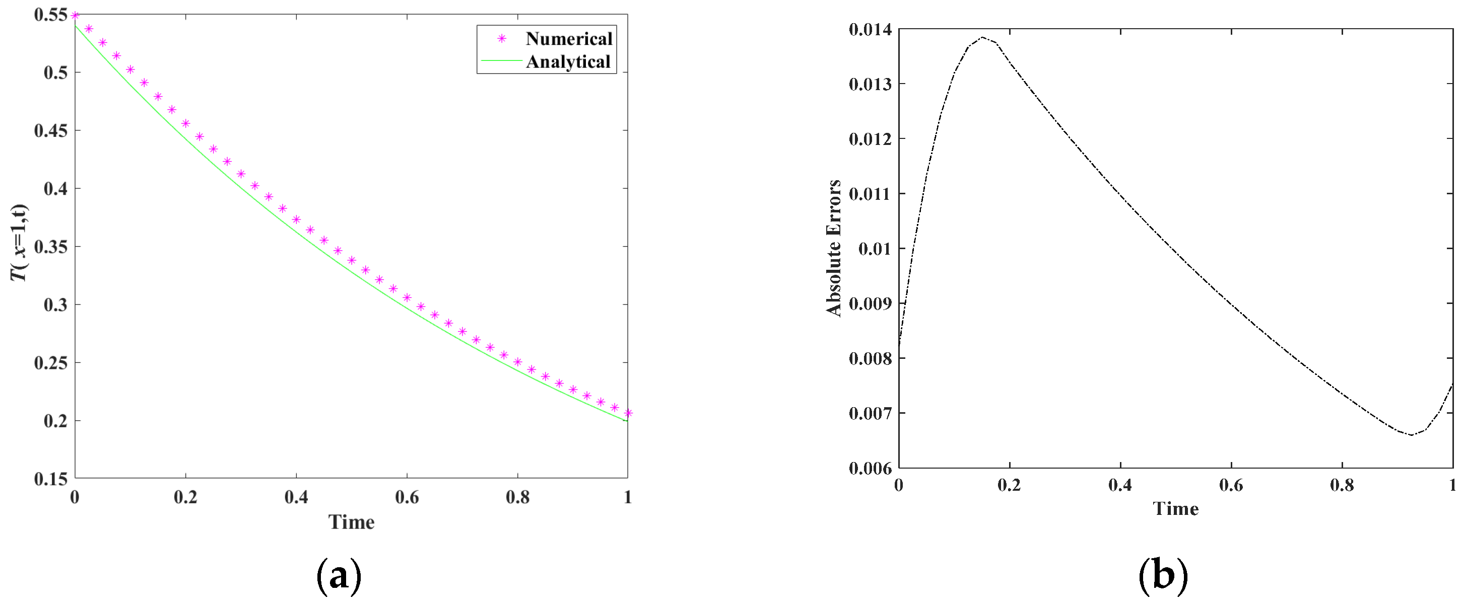
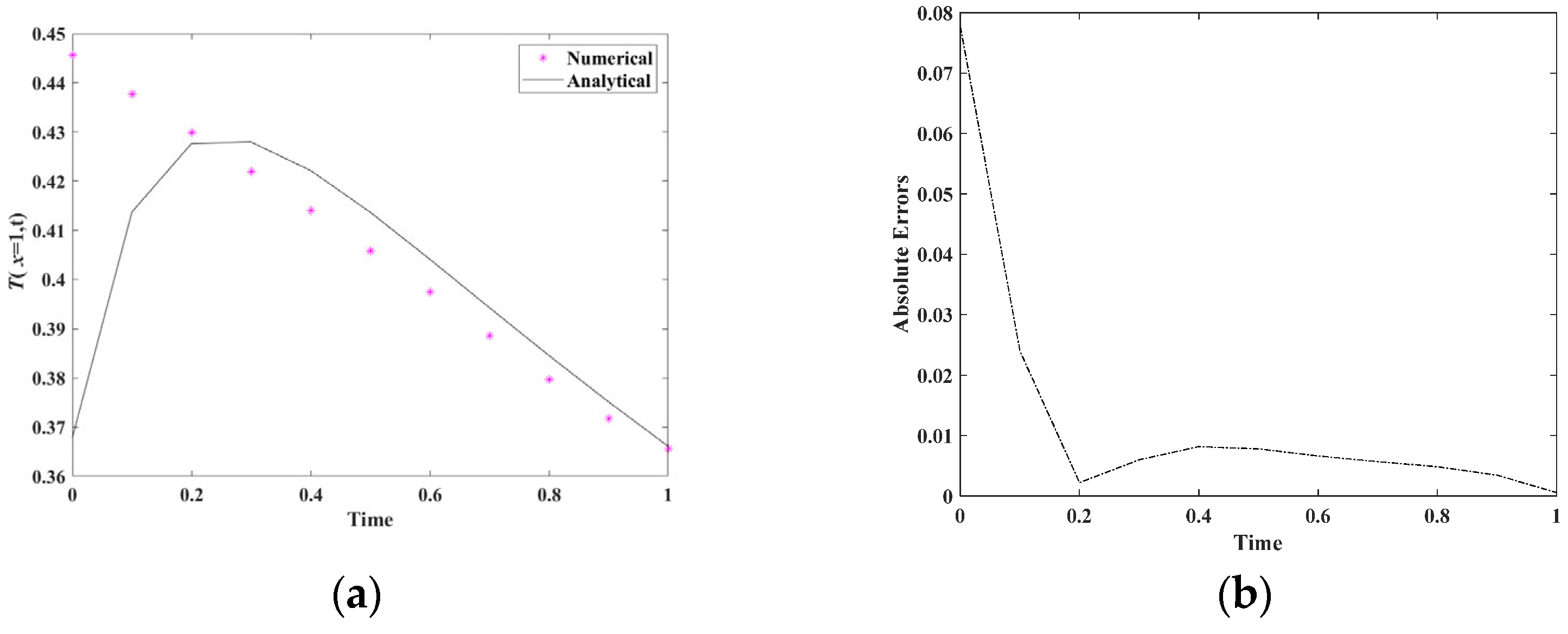
5.2. Example 2
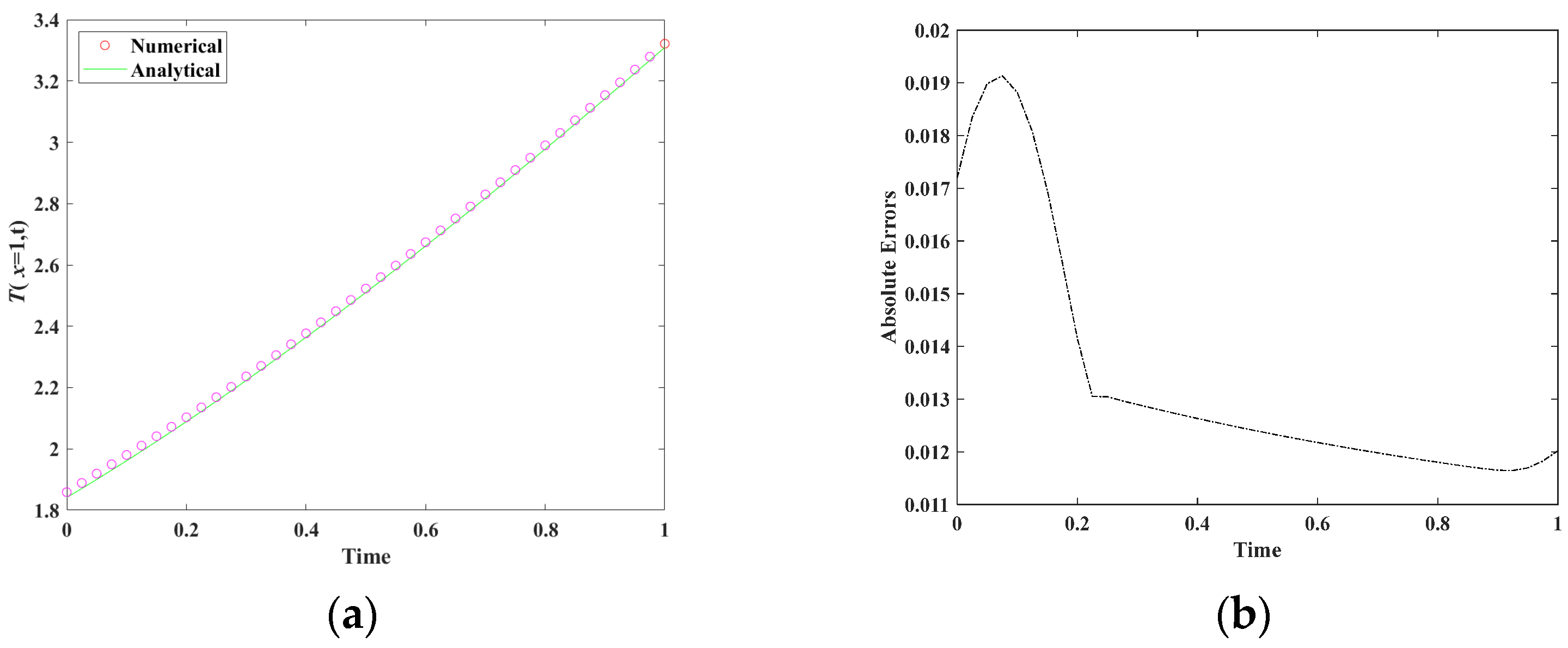
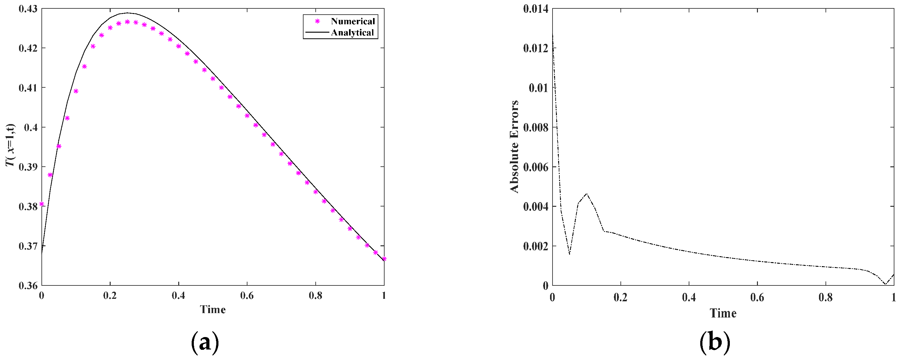
5.3. Example 3
6. Conclusions
Author Contributions
Funding
Data Availability Statement
Conflicts of Interest
References
- Duda, P.; Taler, J. A new method for identification of thermal boundary conditions in water-wall tubes of boiler furnaces. Int. J. Heat Mass Transf. 2009, 52, 1517–1524. [Google Scholar] [CrossRef]
- Maniruzzaman, M.; Sisson, R.D., Jr. Heat transfer coefficients for quenching process simulation. J. Phys. IV 2004, 120, 521–528. [Google Scholar] [CrossRef]
- O’donnell, R.N.; Powell, T.R.; Filipi, Z.S.; Hoffman, M.A. Estimation of thermal barrier coating surface temperature and heat flux profiles in a low temperature combustion engine using a modified sequential function specification approach. J. Heat Transf.-Trans. ASME 2017, 139, 041201. [Google Scholar] [CrossRef]
- Hadamard, J. Lectures on Cauchy’s Problem in Linear Partial Differential Equations; Dover Publications: New York, NY, USA, 1953. [Google Scholar]
- Kronberg, A.E.; Benneker, A.H.; Westerterp, K.R. Notes on wave theory in heat conduction: A new boundary condition. Int. J. Heat Mass Transf. 1998, 41, 127–137. [Google Scholar] [CrossRef]
- Stefanyuk, E.V.; Kudinov, V.A. Approximate analytic solution of heat conduction problems with a mismatch between initial and boundary conditions. Russ. Math. 2010, 54, 55–61. [Google Scholar] [CrossRef]
- Cao, K.; Lesnic, D.; Liu, J. Simultaneous reconstruction of space-dependent heat transfer coefficients and initial temperature. J. Comput. Appl. Math. 2020, 375, 112800. [Google Scholar] [CrossRef]
- Beck, J.V.; Blackwell, B.; St. Clair, C.R. Inverse Heat Conduction: Ill-Posed Problem; Wiley: New York, NY, USA, 1985. [Google Scholar]
- Carasso, A.S. Slowly divergent space marching schemes in the inverse heat conduction problem. Numer. Heat Tranf. B-Fundam. 1993, 23, 111–126. [Google Scholar] [CrossRef]
- Murio, D.A. The mollification method and the numerical solution of the inverse heat conduction problem by finite differences. Comput. Math. Appl. 1989, 17, 1385–1396. [Google Scholar] [CrossRef]
- Murio, D.A. The Mollification Method and the Numerical Solution of Ill-Posed Problems; John Wiley & Sons: New York, NY, USA, 1993. [Google Scholar]
- Al-Khalidy, N. A general space marching algorithm for the solution of two-dimensional boundary inverse heat conduction problems. Numer. Heat Tranf. B-Fundam. 1998, 34, 339–360. [Google Scholar] [CrossRef]
- Eldén, L. Numerical Solution of the Sideways Heat Equation; SIAM: Philadelphia, PA, USA, 1995. [Google Scholar]
- Krutz, G.W.; Schoenhals, R.J.; Horc, P.S. Application of finite element method to the inverse heat conduction problem. Numer. Heat Tranf. B-Fundam. 1978, 1, 489–498. [Google Scholar] [CrossRef]
- Mobtil, M.; Bougeard, D.; Russeil, S. Experimental study of inverse identification of unsteady heat transfer coefficient in a fin and tube heat exchanger assembly. Int. J. Heat Mass Transf. 2018, 125, 17–31. [Google Scholar] [CrossRef]
- Reinhardt, H.J. A numerical method for the solution of two-dimensional inverse heat conduction problems. Int. J. Numer. Methods Eng. 1991, 32, 363–383. [Google Scholar] [CrossRef]
- Brebbia, C.A. Applications of the boundary element method for heat transfer problems. Rev. Gén. Therm. 1985, 24, 353–361. [Google Scholar]
- Pasquetti, R.; Le Niliot, C. Boundary element approach for inverse heat conduction problems: Application to a bidimensional transient numerical experiment. Numer. Heat Tranf. B-Fundam. 1991, 20, 169–189. [Google Scholar] [CrossRef]
- Ingham, D.B.; Yuan, Y.; Han, H. The boundary-element method for an improperly posed problem. IMA J. Appl. Math. 1991, 47, 61–79. [Google Scholar] [CrossRef]
- Kurpisz, K.; Nowak, A.J. BEM approach to inverse heat conduction problems. Eng. Anal. Bound. Elem. 1992, 10, 291–297. [Google Scholar] [CrossRef]
- Lesnic, D.; Elliott, L.; Ingham, D.B. The solution of an in-verse heat conduction problem subject to the specification of energies. Int. J. Heat Mass Transf. 1998, 41, 25–32. [Google Scholar] [CrossRef]
- Al-Najem, N.M.; Osman, A.M.; El-Refaee, M.M.; Khanafer, K.M. Two dimensional steady-state inverse heat conduction problems. Int. Commun. Heat Mass Transf. 1998, 25, 541–550. [Google Scholar] [CrossRef]
- Singh, K.M.; Tanaka, M. Dual reciprocity boundary element analysis of inverse heat conduction problems. Comput. Meth. Appl. Mech. Eng. 2001, 190, 5283–5295. [Google Scholar] [CrossRef]
- Hon, Y.C.; Wei, T. A meshless computational method for solving inverse heat conduction problems. WIT Trans. Model. Simul. 2002, 32, 135–144. [Google Scholar]
- Hon, Y.C.; Wei, T. The method of fundamental solution for solving multidimensional inverse heat conduction problems. CMES-Comp. Model. Eng. Sci. 2005, 7, 119–132. [Google Scholar] [CrossRef]
- Reginska, T. Application of wavelet shrinkage to solving the sideways heat equation. BIT Numer. Math. 2001, 41, 1101–1110. [Google Scholar] [CrossRef]
- Qiu, C.Y.; Fu, C.L.; Zhu, Y.B. Wavelets and regularization of the sideways heat equation. Comput. Math. Appl. 2003, 46, 821–829. [Google Scholar] [CrossRef]
- Berntsson, F. Sequential solution of the sideways heat equation by windowing of the data. Inverse Probl. Eng. 2003, 11, 91–103. [Google Scholar] [CrossRef]
- Cheng, W.; Liu, Y.L.; Yang, F. A modified regularization method for a spherically symmetric inverse heat con-duction problem. Symmetry 2022, 14, 2102. [Google Scholar] [CrossRef]
- Lin, S.M.; Chen, C.K.; Yang, Y.T. A modified sequential approach for solving inverse heat conduction problems. Int. J. Heat Mass Transf. 2004, 47, 2669–2680. [Google Scholar] [CrossRef]
- Zhang, H.; Zou, J.; Xiao, P. Sequential regularization method for the identification of mold heat flux during continuous casting using inverse problem solutions techniques. Metals 2023, 13, 1685. [Google Scholar] [CrossRef]
- Liu, C.S. Cone of non-linear dynamical system and group preserving schemes. Int. J. Non-Linear Mech. 2001, 36, 1047–1068. [Google Scholar] [CrossRef]
- Liu, C.S. Group preserving scheme for backward heat conduction problems. Int. J. Heat Mass Transf. 2004, 47, 2567–2576. [Google Scholar] [CrossRef]
- Liu, C.S.; Chang, C.W.; Chang, J.R. Past cone dynamics and backward group preserving schemes for backward heat conduction problems. CMES-Comp. Model. Eng. Sci. 2006, 12, 67–82. [Google Scholar] [CrossRef]
- Chang, C.W.; Liu, C.S.; Chang, J.R. A new shooting method for quasi-boundary regularization of multi-dimensional backward heat conduction problems. J. Chin. Inst. Eng. 2009, 32, 307–318. [Google Scholar] [CrossRef]
- Chang, J.R.; Liu, C.S.; Chang, C.W. A new shooting method for quasi-boundary regularization of backward heat conduction problems. Int. J. Heat Mass Transf. 2007, 50, 2325–2332. [Google Scholar] [CrossRef]
- Liu, C.S. The Lie-group shooting method for nonlinear two-point boundary value problems exhibiting multiple solutions. CMES-Comp. Model. Eng. Sci. 2006, 13, 149–164. [Google Scholar] [CrossRef]
- Chen, Y.W. A modified Lie-group shooting method for multi-dimensional backward heat conduction problems under long time span. Int. J. Heat Mass Transf. 2018, 127, 948–960. [Google Scholar] [CrossRef]
- Chen, Y.W. A backward-forward Lie-group shooting method for nonhomogeneous multi-dimensional back-ward heat conduction problems under a long time span. Int. J. Heat Mass Transf. 2019, 133, 226–246. [Google Scholar] [CrossRef]
- Chen, Y.W. Simultaneous determination of the heat source and the initial data by using an explicit Lie-group shooting method. Numer. Heat Tranf. B-Fundam. 2019, 75, 239–264. [Google Scholar] [CrossRef]
- Chang, Y.S.; Chen, Y.W.; Liu, C.S.; Chang, J.R. A non-iteration solution for solving the backward-in-time two-dimensional Burgers’ equation with a large Reynolds number. J. Mar. Sci. Technol.-Taiwan 2022, 30, 75–85. [Google Scholar]
- Liu, C.S. An Iterative Method to Recover the Heat Conductivity Function of a Nonlinear Heat Conduction Equation. Numer. Heat Tranf. B-Fundam. 2013, 65, 80–101. [Google Scholar] [CrossRef]
- Liu, C.S. Using a Lie-group adaptive method for the identification of a nonhomogeneous conductivity function and unknown boundary data. CMC-Comput. Mat. Contin. 2011, 21, 17–39. [Google Scholar] [CrossRef]
- Liu, C.S. A Lie-group adaptive method to identify spatial-dependence heat conductivity coefficients. Numer. Heat Tranf. B-Fundam. 2011, 60, 305–323. [Google Scholar] [CrossRef]
- Liu, C.S. An LGEM to identify time-dependent heat conductivity function by an extra measurement of temperature gradient. CMC-Comput. Mat. Contin. 2008, 7, 81–95. [Google Scholar] [CrossRef]


| NT | NS | Maximum Absolute Errors |
|---|---|---|
| 11 | 41 | |
| 101 | ||
| 201 | ||
| 501 | ||
| 41 | 41 | |
| 101 | ||
| 201 | ||
| 501 |
| NT | NS | Maximum Absolute Errors |
|---|---|---|
| 11 | 41 | |
| 101 | ||
| 201 | ||
| 501 | ||
| 41 | 41 | |
| 101 | ||
| 201 | ||
| 501 |
| NT | NS | Maximum Absolute Errors |
|---|---|---|
| 11 | 41 | |
| 101 | ||
| 201 | ||
| 41 | 41 | |
| 101 | ||
| 201 |
Disclaimer/Publisher’s Note: The statements, opinions and data contained in all publications are solely those of the individual author(s) and contributor(s) and not of MDPI and/or the editor(s). MDPI and/or the editor(s) disclaim responsibility for any injury to people or property resulting from any ideas, methods, instructions or products referred to in the content. |
© 2025 by the authors. Licensee MDPI, Basel, Switzerland. This article is an open access article distributed under the terms and conditions of the Creative Commons Attribution (CC BY) license (https://creativecommons.org/licenses/by/4.0/).
Share and Cite
Tan, C.-C.; Shih, C.-F.; Shen, J.-H.; Chen, Y.-W. A Time–Space Numerical Procedure for Solving the Sideways Heat Conduction Problem. Mathematics 2025, 13, 751. https://doi.org/10.3390/math13050751
Tan C-C, Shih C-F, Shen J-H, Chen Y-W. A Time–Space Numerical Procedure for Solving the Sideways Heat Conduction Problem. Mathematics. 2025; 13(5):751. https://doi.org/10.3390/math13050751
Chicago/Turabian StyleTan, Ching-Chuan, Chao-Feng Shih, Jian-Hung Shen, and Yung-Wei Chen. 2025. "A Time–Space Numerical Procedure for Solving the Sideways Heat Conduction Problem" Mathematics 13, no. 5: 751. https://doi.org/10.3390/math13050751
APA StyleTan, C.-C., Shih, C.-F., Shen, J.-H., & Chen, Y.-W. (2025). A Time–Space Numerical Procedure for Solving the Sideways Heat Conduction Problem. Mathematics, 13(5), 751. https://doi.org/10.3390/math13050751