Exploring Chaos and Stability in a 3-D Finance Model with Absolute Function Nonlinearity

Abstract

This paper introduces a novel chaotic finance system derived by incorporating a modeling uncertainty with an absolute function nonlinearity into existing financial systems. The new system, based on the works of Gao and Ma, and Vaidyanathan et al., demonstrates enhanced chaotic behavior with a maximal Lyapunov exponent (MLE) of 0.1355 and a fractal Lyapunov dimension of 2.3197. These values surpass those of the Gao-Ma system (MLE = 0.0904, Lyapunov dimension = 2.2296) and the Vaidyanathan system (MLE = 0.1266, Lyapunov dimension = 2.2997), signifying greater complexity and unpredictability. Through parameter analysis, the system transitions between periodic and chaotic regimes, as confirmed by bifurcation diagrams and Lyapunov exponent spectra. Furthermore, multistability is demonstrated with coexisting chaotic attractors for p = 0.442 and periodic attractors for p = 0.48. The effects of offset boosting control are explored, with attractor positions adjustable by varying a control parameter k, enabling transitions between bipolar and unipolar chaotic signals. These findings underline the system’s potential for advanced applications in secure communications and engineering, providing a deeper understanding of chaotic finance models.

1. Introduction

Studying financial risk systems is crucial for ensuring the stability and sustainability of economic frameworks in an increasingly interconnected global economy [1,2]. Financial markets are inherently dynamic and prone to unpredictable fluctuations due to various factors such as interest rate changes, investment demands, inflation, and external economic shocks [3,4]. Understanding the behavior of financial risk systems, especially chaotic and complex dynamics, allows policymakers, financial institutions, and investors to better anticipate potential crises and mitigate risks [5,6].

To address financial risk systems effectively, a multi-faceted approach must be taken that combines risk identification, assessment, mitigation, and continuous monitoring [7,8]. First, financial institutions and policymakers need to develop advanced models to identify chaotic behavior and nonlinear dynamics in financial systems, which can help predict potential risks and crises [9,10]. Second, implementing robust risk management frameworks, such as stress testing, scenario analysis, and diversification strategies, can help mitigate the impact of financial shocks [11,12]. Third, leveraging technology, such as machine learning and artificial intelligence, can enhance real-time monitoring of financial markets and detect early warning signs of instability [13,14]. Additionally, regulatory bodies must strengthen financial regulations and ensure compliance to reduce systemic risk. Lastly, promoting financial literacy and transparency among market participants is essential to improve decision-making and reduce speculative behavior that could amplify risks [15,16]. By integrating these strategies, financial institutions can better manage uncertainties and maintain the stability of financial systems [17,18].

The challenges in addressing financial risk systems in the future will revolve around the increasing complexity and unpredictability of global financial markets [19]. One major challenge is the rapid advancement of technology, which, while providing new tools for risk management, also introduces new vulnerabilities, such as cyber risks and algorithmic trading failures [20,21]. Additionally, financial systems are becoming more interconnected across borders, making them more susceptible to global economic shocks and contagion effects [22,23]. Regulatory frameworks may struggle to keep pace with the evolving nature of financial innovations, leading to gaps in oversight and risk assessment [24]. Another challenge is the potential for human biases and decision-making errors, particularly in high-pressure environments, which can exacerbate risks [25,26]. Furthermore, the integration of artificial intelligence and machine learning in financial risk management requires careful calibration to avoid over-reliance on automated systems that may fail to account for rare, high-impact events [27,28]. To address these challenges, future approaches must balance technological advancements with strong regulatory oversight, transparency, and a focus on building resilience in financial systems.

In recent decades, there has been significant interest in the financial literature in the modeling of chaotic systems. He et al. [29] conduct a comprehensive theoretical and numerical analysis of the dynamic properties of a financial risk system to enhance the understanding of complex behavior in financial markets. They determined the critical delay value at which Hopf bifurcation occurs by applying the linearization method and Laplace transform. Gao et al. [30] developed a more precise numerical method for analyzing financial systems by incorporating the memory effect of fractional-order derivatives, which better captures the historical significance of financial dynamics. They investigated the system’s dynamic behavior and uncovered novel chaotic attractors by using the Grünwald–Letnikov fractional derivative. Jiao [31] evaluated a financial management early warning model tailored for enterprises operating within a circular economy. By integrating the chaotic particle swarm optimization algorithm with a back-propagation neural network, the study aims to enhance prediction accuracy, improve convergence speed, and establish the model’s effectiveness in ensuring the optimal utilization of financial resources.

Agrawal et al. [32] studied the challenges of financial crises and poverty by developing a deterministic financial system modeled through nonlinear fractional differential equations. By utilizing the Legendre wavelet approximation for the first time in fractional-order financial systems, the research seeks to convert fractional differential equations into algebraic equations, enabling residual, convergence, and stability analyses. Shafiq and Ahmad [33] enhanced financial system stability and economic growth by addressing the challenges posed by chaotic behavior and synchronization issues in financial systems. They developed a novel direct adaptive control strategy that ensures robust synchronization of two identical financial chaoticsystems, despite the presence of unknown exogenous disturbances and model uncertainties.

Asadollahi et al. [34] investigated the understanding and synchronization of new finance systems within the context of an increasingly globalized financial market. They proposed a new prescribed performance control-based sliding mode controller design, ensuring stability and improved performance. Existing studies on chaotic finance systems often lack exploration of mechanisms to flexibly control chaotic attractor positions without altering inherent system dynamics, a limitation addressed in this research through the introduction of offset boosting control in the financial model.

Gao and Ma [35] proposed a new chaotic finance system having two nonlinearities and carried out a detailed bifurcation analysis of the system. Tacha et al. [36] proposed a new chaotic finance system having two nonlinearities (a quadratic nonlinearity and an absolute function nonlinearity) and described a circuit realization of the finance system. Using bifurcation analysis, they investigated the chaotic properties of the finance system and using Lyapunov stability theory, they presented an application of adaptive control for the chaotic finance system.Tacha et al. [37] proposed a new chaotic finance system with dissaving and two nonlinearities (a quadratic nonlinearity and an absolute function nonlinearity) and described a circuit realization of the finance system.Vaidyanathan et al. [38] proposed a new chaotic finance system with two nonlinearities (a quadratic nonlinearity and a quartic nonlinearity) and carried out a detailed bifurcation analysis of the system.

The main contribution and novelty of this work as follows:

• This study presents a new chaotic finance system (7) by introducing an absolute function nonlinearity, which significantly enhances the system’s chaotic behavior compared to existing financial chaotic systems [35,36,37,38]. The proposed system exhibits a higher value of maximal Lyapunov exponent (MLE) and fractal Lyapunov dimension, indicating greater complexity and unpredictability, making it suitable for advanced chaotic applications.
• The work highlights the phenomenon of multistability in the proposed system by demonstrating the coexistence of multiple attractors for specific parameter ranges. This discovery of multistable behavior in a finance system is novel and offers potential for applications in economic models.
• The study introduces offset boosting control to the proposed chaotic finance system, allowing the position of chaotic attractors to be adjusted without altering the system’s inherent dynamics. This feature enables the generation of both bipolar and unipolar chaotic signals, a novel approach with promising applications in economics models.

This work is systematized as follows. Section 2 presents the mathematical formulation of the proposed chaotic finance system, derived by adding a modeling uncertainty term to previous systems. In Section 3, the dynamic behavior of the proposed chaotic finance system is explored in detail using tools such as bifurcation diagrams, Lyapunov exponent spectra, and phase plots. Section 4 investigates the phenomenon of multistability by demonstrating the coexistence of multiple attractors for fixed parameter values and different initial conditions. Section 5 introduces offset boosting control, a novel feature that allows for adjusting the position of chaotic attractors by modifying a control parameter k, enabling transitions between bipolar and unipolar chaotic signals. The paper concludes in Section 6 by summarizing the findings, emphasizing the system’s enhanced complexity and potential applications in the model.

2. A New Finance Chaotic System

Gao and Ma [35] reported a new finance system which has the 3-D dynamics

$$\left\{\begin{array}{l}{\dot{y}}_1=(y_2-a)y_1+y_3\\ {\dot{y}}_2=1-b{y}_2-y_1^2\\ {\dot{y}}_3=-y_1-c{y}_3\end{array}\right.$$

(1)

In the Gao-Ma finance system (1), $y_1$ represents the interest rate, $y_2$ stands for the investment demand and $y_3$ designates the price index. Furthermore, in the financial system (1), the constants $a,b,$ and $c$ represent the financial savings, the investment cost and the commodities demand elasticity, respectively.

Gao and Ma [35] showed that the 3-D financial system (1) has a chaotic attractor, when the parameter values are taken as $a=6,b=0.1,$ and $c=1.$ With the initial state $Y\left(0\right)=\left(0.5,0.3,0.5\right),$ and $\left(a,b,c\right)=\left(6,0.1,1\right),$ the Lyapunov characteristic exponents (LCE) for the Gao-Ma system (1) were calculated for $T=1\times {10}^5$ seconds as follows:

$$l_1=0.0904,l_2=0,l_3=-0.3938$$

(2)

The MLE of the Gao-Ma finance system (1) is $l_1=0.0904.$

Also, the Lyapunov dimension of the Gao-Ma finance system (1) is found as follows:

$$D_L=2+{\displaystyle \frac{1}{\left|l_3\right|}}\left(l_1+l_2\right)=2+{\displaystyle \frac{0.0904}{0.3938}}=2.2296$$

(3)

Tacha et al. [36] modified the Gao and Ma finance system (1) by replacing the quadratic nonlinearity with an absolute function nonlinearity in the second differential equation and obtaining the following finance system:

$$\left\{\begin{array}{l}{\dot{y}}_1=(y_2-a)y_1+y_3\\ {\dot{y}}_2=1-b{y}_2-\left|y_2\right|\\ {\dot{y}}_3=-y_1-c{y}_3\end{array}\right.$$

(4)

In the Tacha finance system (4), the states $y_1,y_2,y_3$ and the parameters $a,b,c$ have the same financial interpretation as in the Gao and Ma finance system (1). Tacha et al. [36] showed that the Tacha finance system (4) has a chaotic attractor when the parameter values are taken as $a=1,b=0.15,$ and $c=1.$

With $Y\left(0\right)=\left(0.5,0.3,0.5\right),$ and $\left(a,b,c\right)=\left(1,0.15,1\right),$ the Lyapunov characteristic exponents (LCE) for the Tacha system (4) were calculated for $T=1\times {10}^5$ s as follows:

$$l_1=0.0646,l_2=0,l_3=-0.4219$$

(5)

The MLE of the Tacha finance system (4) is $l_1=0.0646.$

Also, the Lyapunov dimension of the Tacha finance system (4) is found as follows:

$$D_L=2+{\displaystyle \frac{1}{\left|l_3\right|}}\left(l_1+l_2\right)=2+{\displaystyle \frac{0.0646}{0.4219}}=2.1531$$

(6)

Tacha et al. [37] modified the Gao and Ma finance system (1) by replacing the quadratic nonlinearity with an absolute function nonlinearity in the second differential equation and introducing dissaving in the financial model. Tacha et al. [37] reported the following finance system:

$$\left\{\begin{array}{l}{\dot{y}}_1=(y_2+a)y_1+y_3\\ {\dot{y}}_2=1-b{y}_2-\left|y_2\right|\\ {\dot{y}}_3=-y_1-c{y}_3\end{array}\right.$$

(7)

In the Tacha finance system (4), the states $y_1,y_2,y_3$ and the parameter $a$ stands for dissaving, while the parameters $b,c$ have the same financial interpretation as in the Gao and Ma finance system (1). Tacha et al. [37] showed that the Tacha finance system (7) has a chaotic attractor, when the parameter values are taken as $a=1,b=0.2,$ and $c=1.$

With $Y\left(0\right)=\left(0.5,0.3,0.5\right),$ and $\left(a,b,c\right)=\left(1,0.2,1\right),$ the Lyapunov characteristic exponents (LCE) for the Tacha system (7) were calculated for $T=1\times {10}^5$ seconds as follows:

$$l_1=0.0671,l_2=0,l_3=-0.5366$$

(8)

The MLE of the Tacha finance system (7) is $l_1=0.0671.$

Also, the Lyapunov dimension of the Tacha finance system (7) is found as follows:

$$D_L=2+{\displaystyle \frac{1}{\left|l_3\right|}}\left(l_1+l_2\right)=2+{\displaystyle \frac{0.0671}{0.5366}}=2.1250$$

(9)

Vaidyanathan et al. [38] modified the Gao and Ma finance system (1) by replacing the quadratic nonlinearity with a quartic nonlinearity in the second differential equation and obtaining the following finance system:

$$\left\{\begin{array}{l}{\dot{y}}_1=(y_2-a)y_1+y_3\\ {\dot{y}}_2=1-b{y}_2-y_1^4\\ {\dot{y}}_3=-y_1-c{y}_3\end{array}\right.$$

(10)

In the Vaidyanathan finance system (10), the states $y_1,y_2,y_3$ and the parameters $a,b,c$ have the same financial interpretation as in the Gao and Ma finance system (1). Vaidyanathan et al. [38] showed that the finance system (10) has a chaotic attractor when the parameter values are taken as $a=7,b=0.1,$ and $c=1.$

With $Y\left(0\right)=\left(0.5,0.3,0.5\right),$ and $\left(a,b,c\right)=\left(7,0.1,1\right),$ the Lyapunov characteristic exponents (LCE) for the Vaidyanathan system (10) were calculated for $T=1\times {10}^5$ seconds as follows:

$$l_1=0.1266,l_2=0,l_3=-0.4224$$

(11)

The MLE of the Vaidyanathan finance system (4) is $l_1=0.1266.$

Also, the Lyapunov dimension of the Vaidyanathan finance system (3) is found as follows:

$$D_L=2+{\displaystyle \frac{1}{\left|l_3\right|}}\left(l_1+l_2\right)=2+{\displaystyle \frac{0.1266}{0.4224}}=2.2997$$

(12)

In this research work, we obtain a new chaotic financial system by adding a modeling uncertainty with an absolute function nonlinearity into the finance chaotic system (10). Tacha et al. [36] noted that from the economic theory point of view, the changing rate of the investment demand is in proportion to the interest rate $y_1,$ and they have adopted the use of an absolute function nonlinearity $-\left|y_1\right|$ in the differential equation for $y_2.$

Thus, our new finance system is given by the following 3-D dynamics:

$$\left\{\begin{array}{l}{\dot{y}}_1=(y_2-a)y_1+y_3\\ {\dot{y}}_2=1-b{y}_2-p\left|y_1\right|-y_1^4\\ {\dot{y}}_3=-y_1-c{y}_3\end{array}\right.$$

(13)

In the new system (13), the states $y_1,y_2,y_3$ and the parameters $a,b,c$ have the same financial interpretation as in the Gao and Ma finance system (1) and the Vaidyanathan finance system (10). We will show that the new chaotic finance system (7) has a chaotic attractor, when the parameter values are taken as $a=6.8,b=0.1,c=1$ and $p=0.1.$

With $Y\left(0\right)=\left(0.5,0.3,0.5\right),$ and $\left(a,b,c,p\right)=\left(6.8,0.1,1,0.1\right),$ the Lyapunov characteristic exponents (LCE) for the new finance system (13) were calculated for $T=1\times {10}^5$ s as follows:

$$l_1=0.1355,l_2=0,l_3=-0.4239$$

(14)

The maximal Lyapunov exponent (MLE) of the new chaotic finance system (13) is $l_1=0.1355.$

Also, the Lyapunov dimension of the new chaotic finance system (13) is found as follows:

$$D_L=2+{\displaystyle \frac{1}{\left|l_3\right|}}\left(l_1+l_2\right)=2+{\displaystyle \frac{0.1355}{0.4239}}=2.3197$$

(15)

It is thus observed that the new chaotic finance system (13) has a greater value of the fractal Lyapunov dimension than that of the Gao-Ma chaotic finance system (1), the Tacha finance system (4), the Tacha finance system with dissaving (7), and the Vaidyanathan financial system (10). Moreover, we note that the MLE of the new chaotic finance system (13) is greater than the MLE of the Gao-Ma chaotic finance system (1), the Tacha chaotic finance system (4), the Tacha chaotic finance system with dissaving (7) and the Vaidyanathan finance system (10). We have summarized our comparison results in

Table 1. Comparison of Maximal Lyapunov Exponent (MLE) and Lyapunov Dimension ($D_L$) for Five Chaotic Finance Systems.

System	Maximal Lyapunov Exponent	Lyapunov Dimension (${\mathit{D}}_{\mathit{L}}$)
Gao-Ma Finance System [35]	$0.0904$	$2.2296$
Tacha Finance System [36]	$0.0646$	$2.1531$
Tacha Finance System [37]	$0.0671$	$2.1250$
Vaidyanathan System [38]	$0.1266$	$2.2997$
New Finance System	$0.1355$	$2.3197$

.

For the new chaotic finance system (13), we fix the parameter values as in the chaotic case, viz. $\left(a,b,c,p\right)=\left(6.8,0.1,1,0.1\right).$ A simple calculation shows that the system (13) has two rest points given by $P_1=\left(0,10,0\right)$ and $P_2=\left(0.6295,7.8000,-0.6295\right).$

The Jacobian matrix of the system (13) at $P_1$ has the eigenvalues $-0.1,-0.7466$ and $2.9466,$ which shows that $P_1$ is an unstable, saddle rest point. Also, the Jacobian matrix of the system (13) at $P_2$ has the eigenvalues $-0.6552$ and $0.2776\pm 0.9888i,$ which shows that $P_2$ is an unstable, saddle-focus, rest point.

The phase plots of the new chaotic system (13) for the initial state (0.5, 0.3, 0.5) and the parameter values $\left(a,b,c,p\right)=\left(6.8,0.1,1,0.1\right)$ are shown in the Figure 1.

3. Exploring the Dynamics of the System

In this section, the dynamic behavior of the new chaotic finance system (13) is thoroughly analyzed in relation to changes in its parameters and initial points. This investigation is carried out by employing several tools, including Lyapunov exponents (LE)spectra, bifurcation diagrams, and phase plots, to provide a comprehensive understanding of how the system evolves under varying conditions. Throughout this section, the initial state of the new chaotic finance system (7) is taken as $Y\left(0\right)=\left(0.5,0.3,0.5\right).$

3.1. Parameter $a$ Variation and Its Effect on System Dynamics

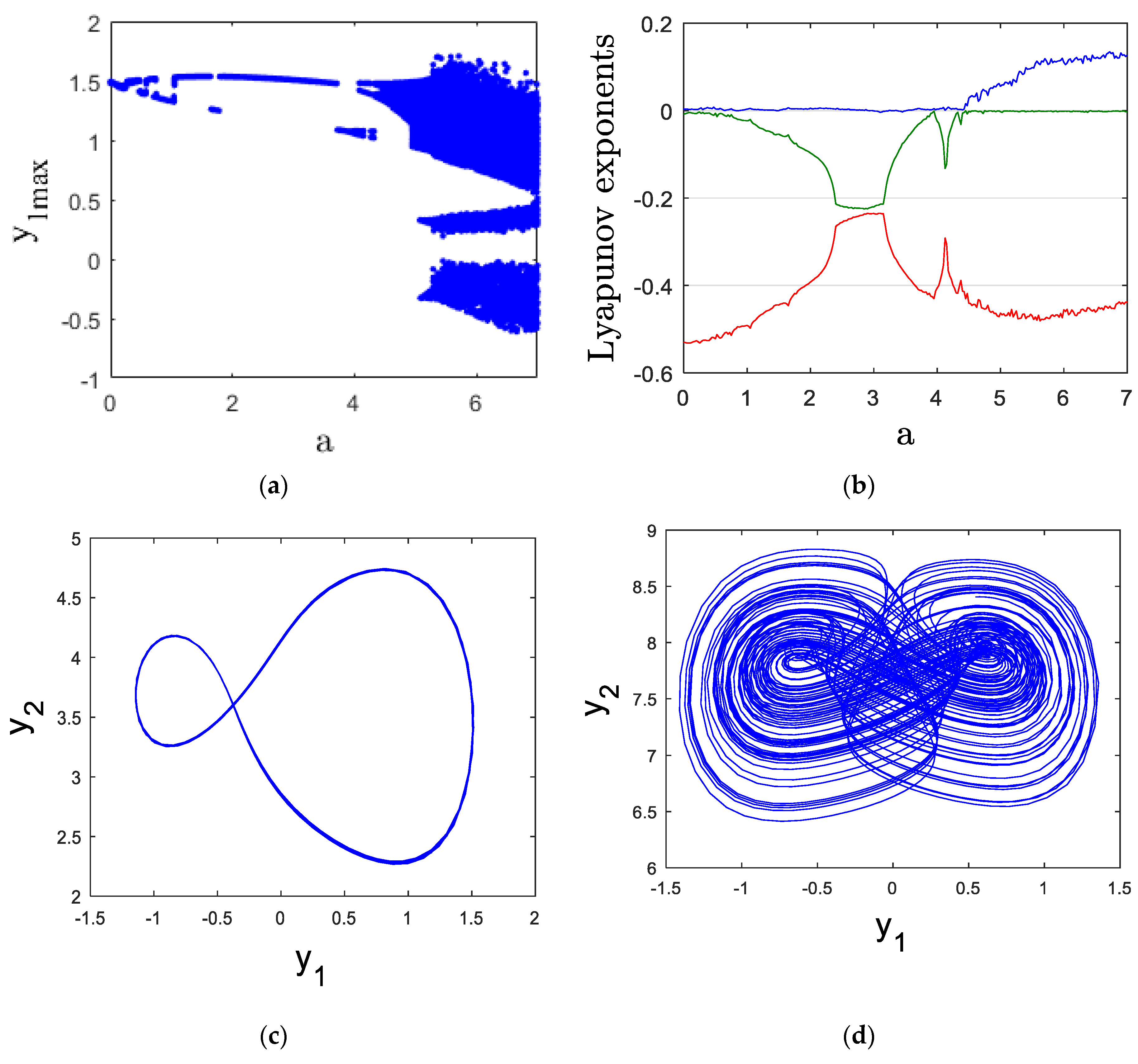
In this section of the analysis, we investigate the impact of the parameter $a$ on the system’s dynamics by varying it within the range of 0 to 7. To illustrate the effects, we employ bifurcation diagrams and the Lyapunov exponent spectrum, as presented in Figure 2a,b. The results indicate that the new chaotic finance system (13) exhibits both periodic and chaotic behavior, depending on the values of $a.$

When the parameter $a$ lies within the interval [0, 4.4], the system displays periodic dynamics, as shown in Figure 2a. This is further supported by the observation of a zero maximal Lyapunov exponent (MLE) in this range, as depicted in Figure 2b. For a more detailed view, Figure 1c shows the periodic orbit at a = 3, with the corresponding Lyapunov exponents: LE₁ = 0, LE₂ = −0.220, and LE₃ = −0.326.

In contrast, for the values of $a$ in the interval [4.4, 7], the system undergoes a transition to chaotic behavior, as shown in Figure 2a. The presence of chaos is confirmed by a positive MLE in this range, as evidenced in Figure 2b. To illustrate this chaotic regime more clearly, Figure 1d displays the chaotic attractor at $a$ = 7, with the Lyapunov exponents LE₁ = 0.127, LE₂ = 0, and LE₃ = −0.438.

Financial savings play a crucial role in both chaotic and periodic financial systems, influencing economic stability and market behavior. In a chaotic financial system, savings may fluctuate unpredictably due to external shocks, interest rate volatility, and rapid changes in investment demand, leading to instability in economic growth and capital allocation. This unpredictability can result in financial crises, as seen in periods of excessive speculative investments followed by sudden liquidity shortages. On the other hand, in a periodic financial system, savings follow a more structured and predictable pattern, promoting steady capital accumulation and investment cycles. This stability allows for better risk management, long-term financial planning, and sustainable economic growth.

3.2. Parameter $b$ Variation and Its Effect on System Dynamics

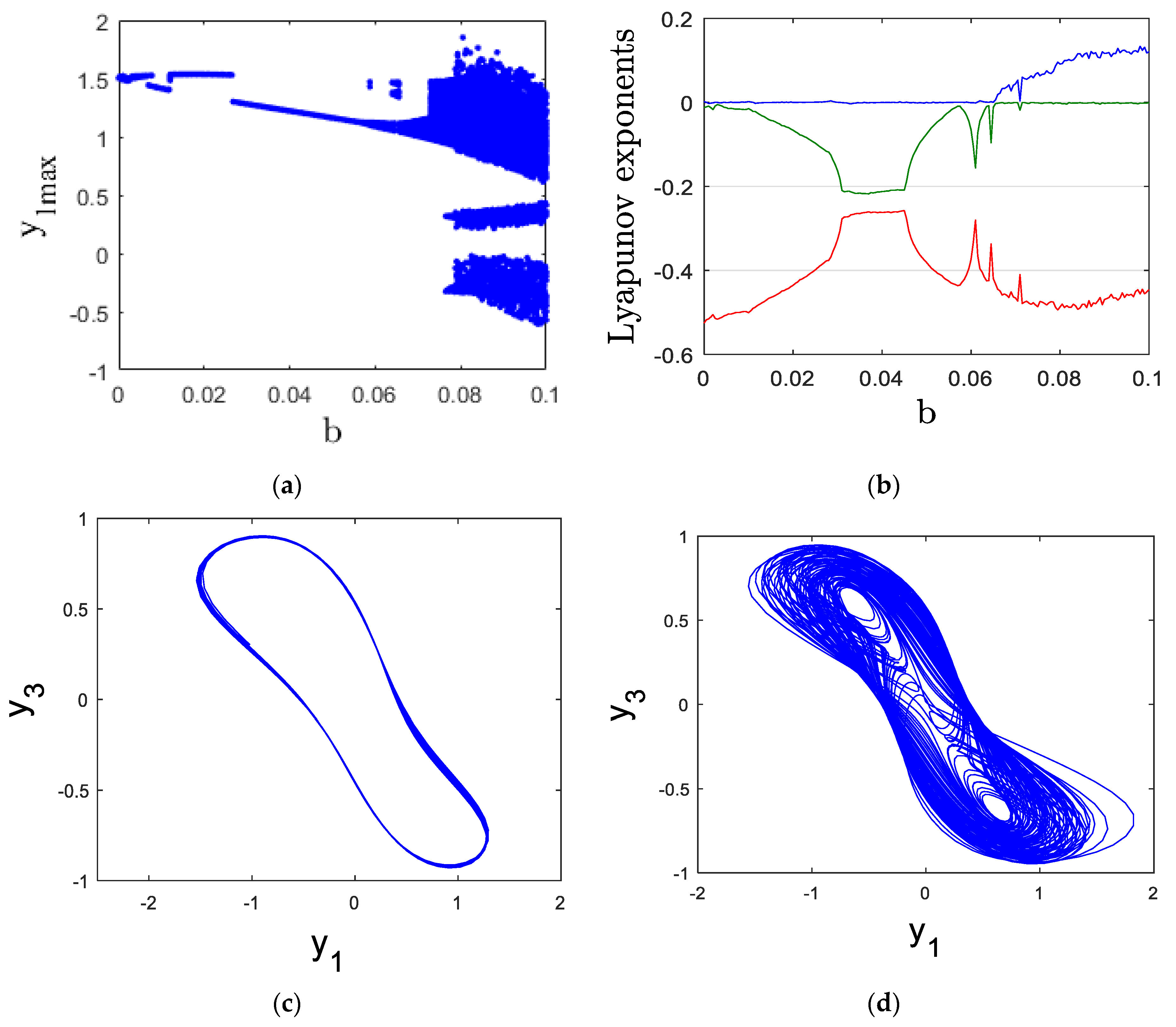
In this subsection, we investigate how variations in the parameter $b$ within the range [0, 0.1] influence the dynamics of the system. The bifurcation diagram and Lyapunov exponent spectrum are used for analysis, as shown in Figure 3a,b.

For the values of $b$ in the interval [0, 0.065], the system (13) exhibits periodic behavior, which is confirmed by a zero MLE as observed in Figure 3b. For further clarification, consider the periodic attractor at $b$ = 0.03, where the corresponding Lyapunov exponents are LE₁ = 0, LE₂ = −0.162, and LE₃ = −0.326 (Figure 3c).

When the parameter $b$ is within the range [0.065, 0.1], the system transitions into chaotic behavior, which is evident in the bifurcation diagram (Figure 3a) and supported by the positive MLE in Figure 3b. The chaotic attractor at $b$ = 0.09, shown in Figure 3d, has Lyapunov exponents LE₁ = 0.116, LE₂ = 0, and LE₃ = −0.469.

Investment cost significantly influences both chaotic and periodic financial systems, shaping capital flow and economic stability. In a chaotic financial system, high investment costs can amplify instability by discouraging businesses from making long-term investments, leading to erratic economic cycles and unpredictable market behavior. This uncertainty can result in abrupt expansions and contractions in financial markets, increasing the risk of financial crises. Conversely, in a periodic financial system, investment costs tend to follow a more structured pattern, allowing firms to plan and allocate resources more efficiently. Moderate and stable investment costs encourage steady capital formation, fostering economic growth and minimizing financial turbulence. However, excessively low investment costs in a periodic system may lead to overinvestment and asset bubbles, while excessively high costs can suppress entrepreneurial activities and slow economic progress. Balancing investment costs is crucial to maintaining a stable yet dynamic financial environment, ensuring sustainable growth without excessive volatility.

3.3. Parameter $c$ Variation and Its Effect on System Dynamics

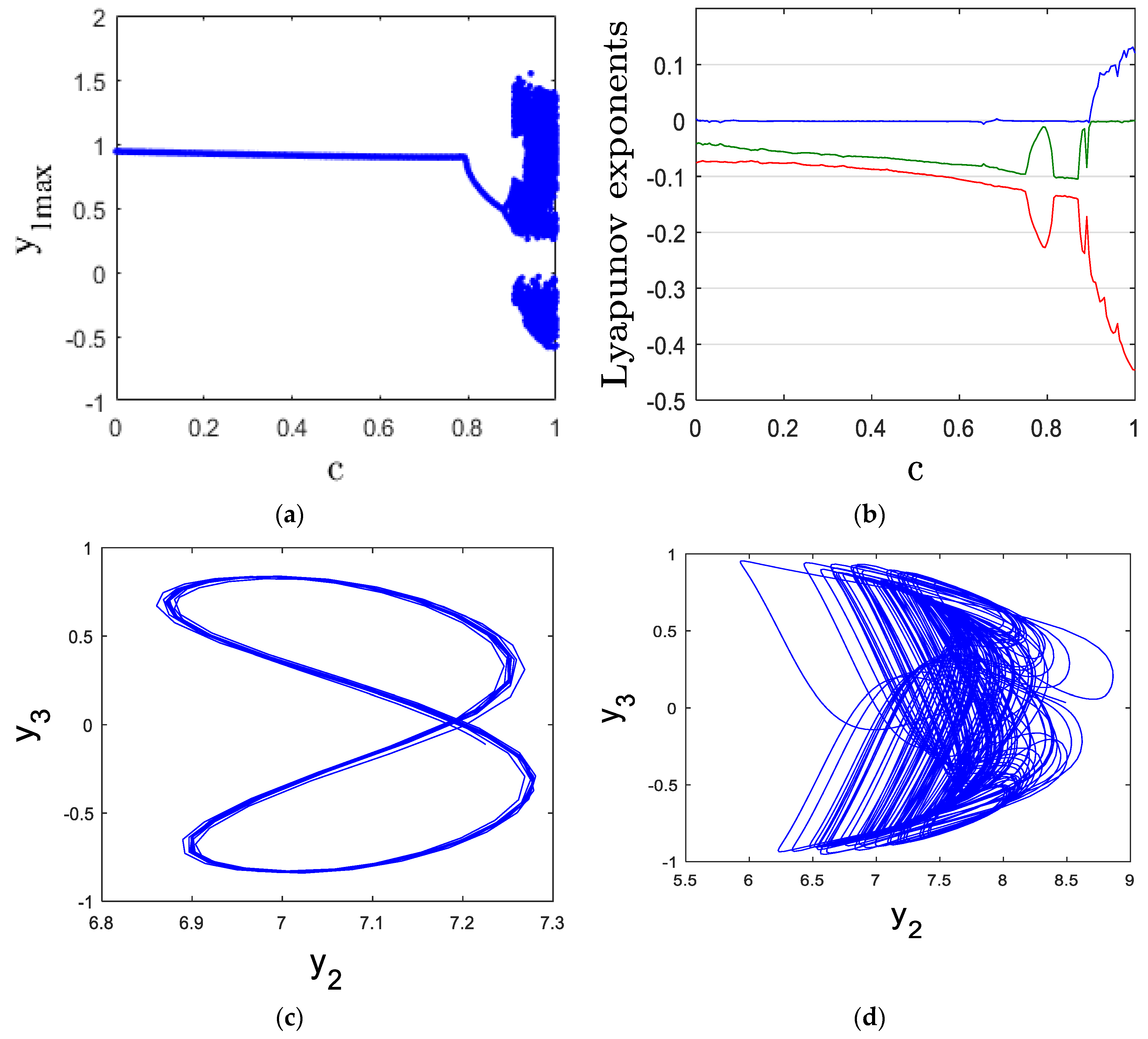
This subsection examines the effect of the parameter $c$, varying between 0 and 1, on the system’s dynamics. The bifurcation diagram (Figure 4a) and Lyapunov exponent spectrum (Figure 4b) offer a detailed analysis of these changes.

When the parameter $c$ is in the range [0, 0.895], the system behaves periodically, as seen in Figure 4a. This periodicity is further supported by the zero MLE observed in Figure 4b. Figure 4c presents the periodic attractor at $c$ = 0.3, with the corresponding Lyapunov exponents: LE₁ = 0, LE₂ = −0.060, and LE₃ = −0.081.

However, for the values of $c$ within the interval [0.895, 1], the system undergoes a shift to chaotic behavior. This transition is confirmed by the positive MLE in Figure 4b. Figure 4d shows the chaotic attractor at $c$ = 0.95, with Lyapunov exponents LE₁ = 0.100, LE₂ = 0, and LE₃ = −0.380.

Commodities’ demand elasticity plays a crucial role in shaping the behavior of both chaotic and periodic financial systems by influencing price stability and market dynamics. In a chaotic financial system, high demand elasticity can amplify fluctuations, as small changes in prices lead to significant shifts in demand, creating instability in production, supply chains, and financial markets. This volatility can contribute to unpredictable price swings, speculative bubbles, and financial crises, as seen in highly reactive commodity markets like oil and agricultural products. On the other hand, in a periodic financial system, demand elasticity follows a more structured pattern, allowing businesses to anticipate changes in demand and adjust production and pricing strategies accordingly. Low elasticity in a periodic system results in stable markets, as demand remains relatively unaffected by price variations, leading to predictable investment and financial planning. However, if demand elasticity is too low, markets may become rigid, reducing adaptability to economic changes and potentially leading to inefficiencies in resource allocation. Striking a balance in demand elasticity is vital to ensuring financial stability while maintaining market responsiveness.

3.4. Parameter $p$ Variation and Its Effect on System Dynamics

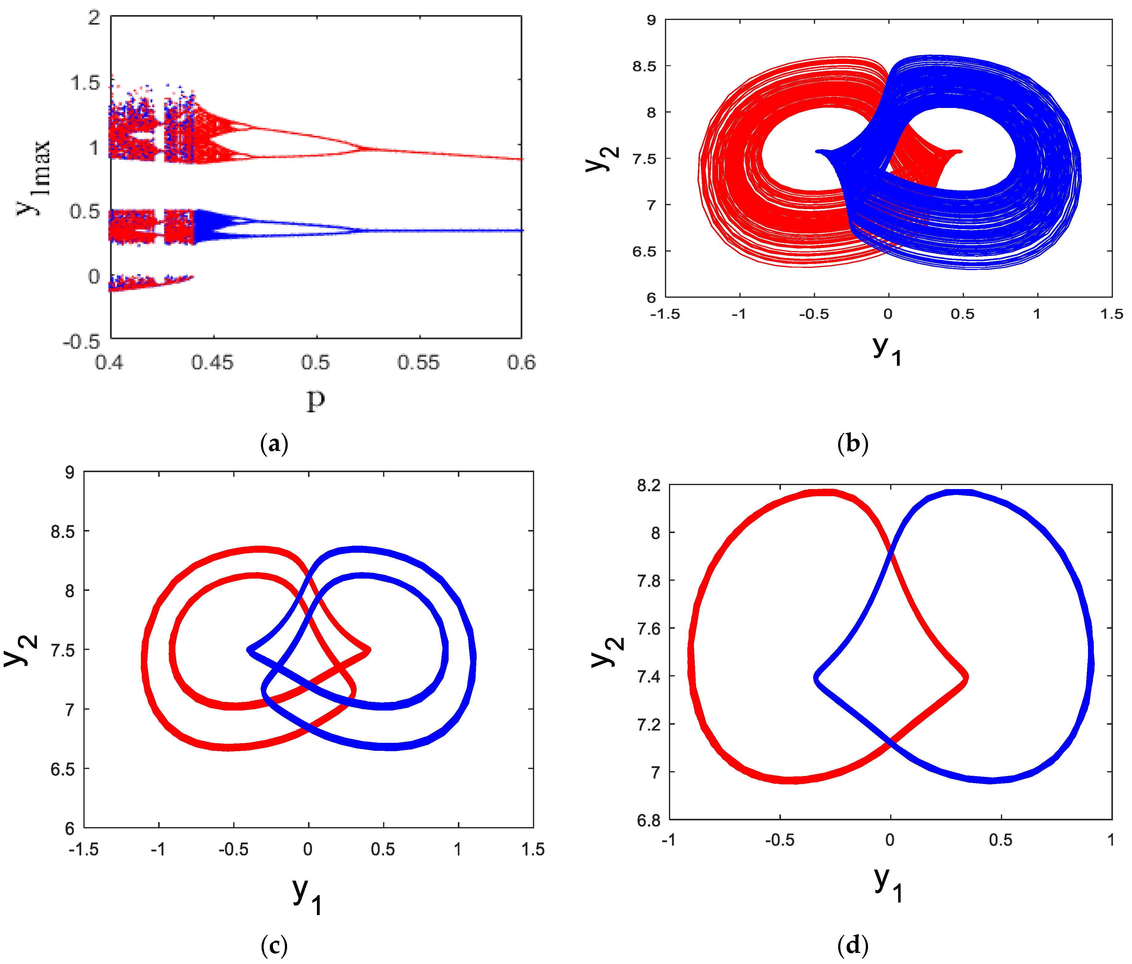
This subsection explores how variations in the parameter $p$ between 0.1 and 1 affect the system’s dynamics. The bifurcation diagram (Figure 5a) and the Lyapunov exponent spectrum (Figure 5b) provide key insights into these changes.

For the values of $p$ in the intervals [0.1, 0.34] and [0.36, 0.46], the system (13) exhibits chaotic behavior, as indicated by the positive maximal Lyapunov exponent (MLE) shown in Figure 5b. To visualize this, Figure 5c illustrates the chaotic attractor at $p$ = 0.3, with Lyapunov exponents LE₁ = 0.082, LE₂ = 0, and LE₃ = −0.391.

On the other hand, for the values of $p$ in the ranges [0.34, 0.36] and [0.46, 1], the system shifts to periodic behavior. This transition is visible in the bifurcation diagram (Figure 5a) and is supported by the zero MLE in Figure 5b. Figure 5d shows the periodic attractor at $p$ = 0.8, with corresponding Lyapunov exponents LE₁ = 0, LE₂ = −0.140, and LE₃ = −0.187.

Market Adjustment Sensitivity, represented by parameter p, plays a critical role in determining the stability and responsiveness of financial systems. In a chaotic financial system, high market adjustment sensitivity can lead to excessive volatility, where small economic changes trigger disproportionate shifts in interest rates, investment demand, and price indices. This heightened sensitivity amplifies market unpredictability, potentially causing abrupt financial crises, speculative bubbles, or sudden collapses. Conversely, in a periodic financial system, moderate market adjustment sensitivity allows for smoother transitions between economic cycles, ensuring that financial markets respond in a controlled and predictable manner to external and internal factors.

4. Coexistence of Multiple Attractors and Multistable Behavior

Multistability is a crucial concept in nonlinear dynamics, where a multistable chaotic system can produce multiple coexisting attractors for fixed parameter values and varying initial conditions. This phenomenon provides significant flexibility for engineering applications based on chaotic systems. To demonstrate that the proposed new chaotic finance system (13) exhibits multistability, we present the bifurcation diagram of the system in relation to the parameter $p$ for two distinct initial conditions.

The bifurcation diagram of the new chaotic finance system (13) for two different initial points is shown in Figure 6a, with $p$ varying between [0.4, 0.6]. The blue trajectory corresponds to the initial point Y₀₁, and the red trajectory corresponds to Y₀₂. It is evident from the diagram that coexisting attractors exist. To further illustrate this, Figure 6b displays two coexisting chaotic attractors at $p$ = 0.442, Figure 6c shows two coexisting period-2 attractors at p = 0.48, and Figure 6d presents two coexisting period-1 attractors at $p$ = 0.58.

5. Effect of Offset Boosting Control on System Dynamics

Offset boosting control provides a versatile method for adjusting the amplitude of a system (13) by incorporating a feedback state. While this technique does not modify the system’s inherent dynamics, it allows for the shifting of the attractor’s position either positively or negatively, depending on the value of the control parameter.

In the newly proposed chaotic finance system (13), variable-boosting chaotic behavior is exhibited, with the ability to adjust y₃. Specifically, y₃ can be enhanced by replacing it with y₃ + k in the system’s equations. Thus, we get the modified dynamical system as follows:

$$\left\{\begin{array}{l}{\dot{y}}_1=(y_2-a)y_1+(y_3+k)\\ {\dot{y}}_2=1-b{y}_2-p\left|y_1\right|-y_1^4\\ {\dot{y}}_3=-y_1-c(y_3+k)\end{array}\right.$$

(16)

The phase portraits of the y₁–y₃ attractor for the modified dynamical system (10) are shown in Figure 7. When the parameter $k$ is negative, the attractors are shifted in the positive direction, whereas a positive $k$ results in a shift in the negative direction. This approach enables the chaotic signal y₃ to transition from a bipolar to a unipolar chaotic signal. This distinctive feature holds considerable promise for applications in secure communications and various engineering fields.

6. Conclusions

This study introduced a new chaotic finance system (13) by incorporating an absolute function nonlinearity into existing financial models. The newly proposed system demonstrated enhanced chaotic behavior compared to the Gao-Ma, Tacha, and Vaidyanathan financial systems, with a higher Maximal Lyapunov Exponent (MLE) and fractal Lyapunov dimension, indicating increased complexity and unpredictability. The dynamic analysis revealed that the system exhibits a rich variety of behaviors, transitioning between periodic and chaotic regimes depending on parameter variations.

The investigation of multistability further highlighted the system’s potential for generating multiple coexisting attractors under fixed parameter values, offering significant flexibility for practical applications, particularly in secure communications. Additionally, the effect of offset boosting control on the system’s dynamics was explored, demonstrating its capacity to shift chaotic attractors, which could be useful for engineering applications involving chaotic signal modulation.

In conclusion, this novel chaotic finance system provides new insights into financial dynamics, enhancing the understanding of chaotic behaviors in economic models. The system’s ability to exhibit multistability and offset-boosting control presents promising applications in secure data transmission, cryptography, and other engineering fields. Future research could focus on further extending this model by incorporating fractional-order derivatives or exploring synchronization techniques to improve its applicability in real-world financial systems.