Abstract
The so-call SQUIDs (abbreviated from superconducting quantum interference device) are very sensitive apparatuses especially built for metering very low magnetic fields. These systems have applications in various practical fields—biology, geology, medicine, different engineering areas, etc. Their features are mainly based on superconductors and the Josephson effect. They can be differentiated into two main groups—direct current (DC) and radio frequency (RF) SQUIDs. Both of them were constructed in the 1960s at Ford Research Labs. The main difference between them is that the second ones use only one superconducting tunnel junction. This reduces their sensitivity, but makes them significantly cheaper. We investigate namely the rf-SQUIDs in the present work. A number of authors devote their research to the rf-SQUIDs driven by an oscillating external flux. We aim to enlarge the theoretical base of these systems by adding new factors in their dynamics. Several particular cases are explored and simulated. We demonstrate also some specialized modules for investigating the proposed model. One application for possible control over oscillations is also discussed. It is based on the Fourier transform and, as a consequence, on the characteristic function of some probability distributions.
Keywords:
homoclinic and heteroclinic bifurcations in rf SQUIDs; Melnikov function; control over oscillations MSC:
34C37
1. Introduction
A number of authors devote their research to the rf superconducting quantum interference device (SQUID) driven by an oscillating external flux.
Direct current (DC) and radio frequency (RF) SQUIDs were constructed in the 1960s at Ford Research Labs—we refer to the original work [1] as well as to the seminal handbooks [2,3]. The reader can find detailed information about the odd and even subharmonics and chaos in rf SQUIDS and about homoclinic and heteroclinic bifurcations in rf SQUIDs in the leading studies [4,5,6,7,8,9,10,11,12]. We will explicitly note the important research related to the following: odd and even subharmonics and chaos in rf SQUIDS [4]; chaotic dynamics of periodically driven rf SQUIDs [5]; homoclinic and heteroclinic bifurcations in rf SQUIDs [6,7]; Melnikov’s method at a saddle-node [8,9]; and the dynamics of the forced Josephson junction [10]. Other interesting problems are discussed in [11,12]. The basic monographs [2,3] cited above provide a relatively complete bibliography on the subject under consideration. We will mention just some of the leading research on the following topics: theory of the signal transfer and noise properties of the rf SQUID [13,14,15,16,17,18,19,20]; SQUIDs and their applications [13,20,21,22,23,24,25]; performance factors in rf SQUIDs—high frequency limit [26,27,28,29,30]; signal characteristics for high Tc rf SQUID [31,32,33]. Some of the latest results concerning the control problems with real applications can be found in [34,35].
The dimensionless equations of motion for the rf SQUID can be written in the form (see, for example, [12]):
where .
Evidently, this system is time-independent Hamiltonian with
and the energy potential is
Depending upon the potential parameter c, there may exist a great variety of separatrix solutions and associated hyperbolic fixed points in the phase space of (1) (for ).
One obtains the hyperbolic fixed points from the conditions
Because the unperturbed system contains both heteroclinic and homoclinic orbits, the different cases are treated separately.
At first in [12], the author consider the case of an upper heteroclinic solution.
From (1), (2) one obtains
The Melnikov function [36] is given by (see, for example, [12]):
where
In this paper, we suggest a new modified model.
Several simulations are composed. We demonstrate also some specialized modules for investigating the dynamics of these hypothetical oscillators.
The derived results can be used as an integral part of a much more general application for scientific computing—for some details, see [37,38,39,40].
2. A New Model: Some Simulations
We consider the following new modified model of the form:
where , , and N is integer.
We note that the Melnikov function [36] corresponding to Model (4) is of the form
The study of the dynamics of such models and the explicit representation of the Melnikov function can be done in the way described, for example, in [12] and in the previous Section 1, and we will omit it here.
Bruhn and Koch discussion [12] shows that the Melnikov method can successfully be applied to systems with complicated potentials, for which an analytic calculation of the associated integrals is not possible.
The expense in numerical calculation is relatively low, so the authors [12] recommend the numerical implementation of the Melnikov method, to determine parameter regions of complicated behaviour.
Because of the complicated potential the resulting integrals have to be evaluated numerically (for example, applying a fourth order Runge–Kutta method). However, we note that Runge–Kutta methods are not symplectic, so they are not suited well for simulating Hamiltonian and chaotic systems. There are several modern ODE solvers, see [41,42,43] as alternatives, namely, semi-implicit CD methods, which are suitable for boundary value problems, as well as the semi-explicit midpoint method and composition semi-implicit schemes based on Suzuki/Yoshida/Suzuki-Trotter or Casas formulas. Otherwise, the numerical effects may affect the results of analysis, and some features can be suppressed (see [44]) or induced (see [45] on inducing multistability in initially monostable systems), which may confuse the final results of the study. The reader can find additional bibliography on numerical methods for chaotic ODE in [46].
We will look at some interesting simulations on Model (4):
Example 1.
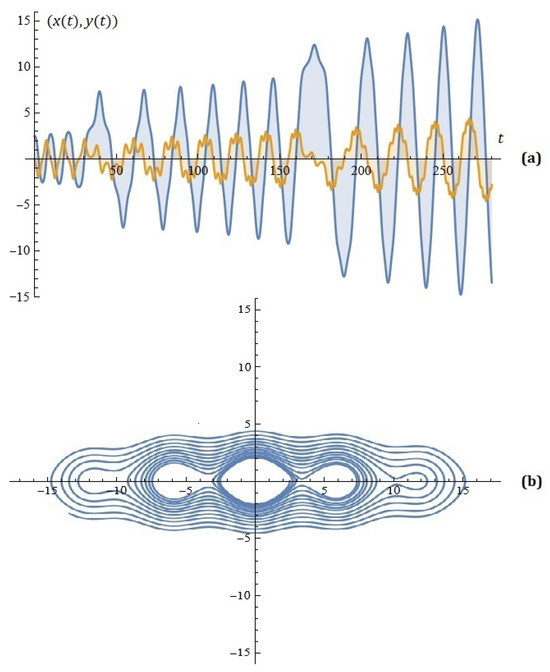
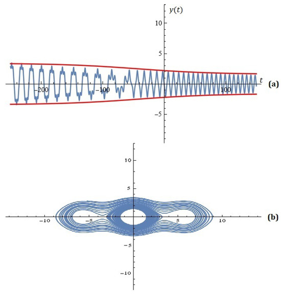
Given , , , , , , , , and , the simulations on the system (4) for ; are depicted on Figure 1.
Figure 1.
(a) The solutions of the system (4); (b) phase space (Example 1).
Example 2.
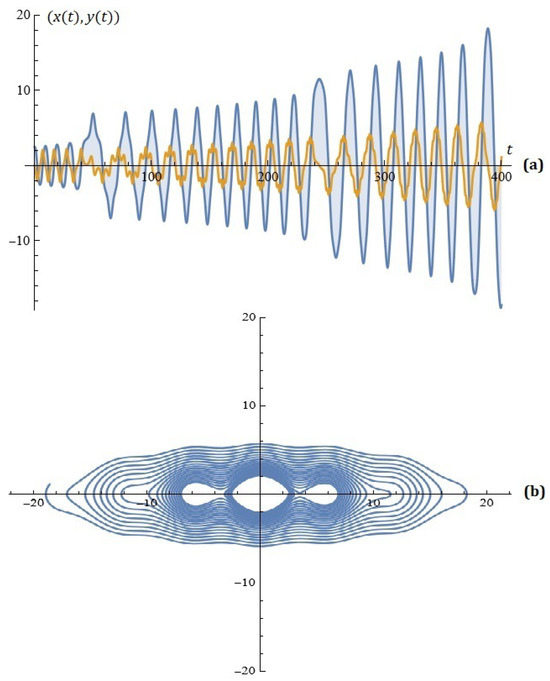
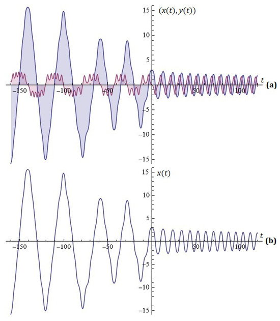
Given , , , , , , , , , , and , the simulations on the system (4) for ; are depicted on Figure 2.
Figure 2.
(a) The solutions of the system (4); (b) phase space (Example 2).
Example 3.
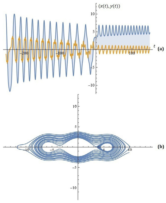
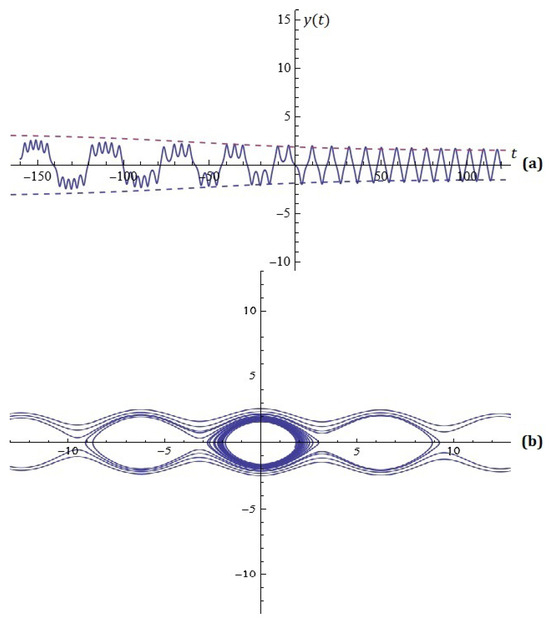
Given , , , , , , , , , , and , the simulations on the system (4) for ; are depicted on Figure 3.
Figure 3.
(a) The solutions of the system (4); (b) phase space (Example 3).
3. Possible Control over Oscillations
3.1. Approximation with Restrictions
The new Model (4) has many free parameters that make it attractive for engineering calculations, for example for possible oscillation control—a user-preset level (or fork) for the oscillations of the y-component of the differential system solution. Suppose that we need to constrain the oscillator in the interval , where the function is of the type (the most common constraint)
Therefore, once we define the oscillator by the parameters c, , b, , N, , and the initial condition , we need to find these values of that minimize the distance between the y-component and the functions and .
Example 4.
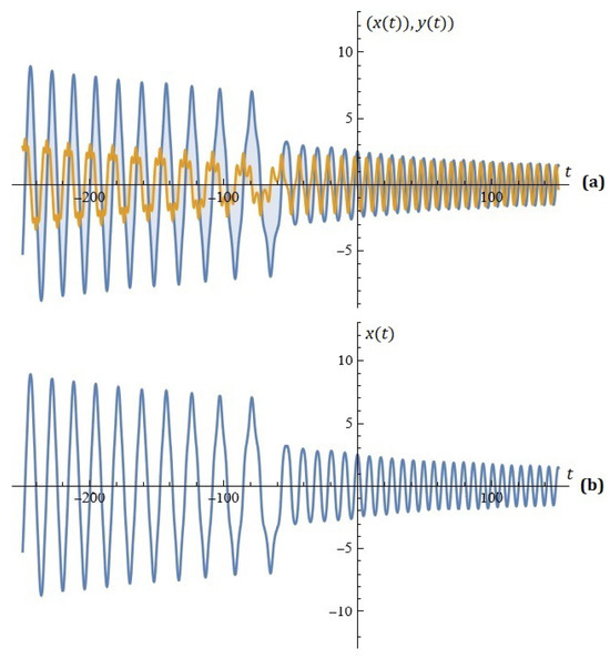
Given , , , , , , , and , it turns out that the optimal values for are , , , and . The simulations on the system (4) together with the constraints are depicted on Figure 4 and Figure 5.
Figure 4.
(a) The solutions of the system (4); (b) component of solution (Example 4).
Figure 5.
(a) component of solution with restrictions (6); (b) phase space (Example 4).
Example 5.
Given , , , , , , , , , , , , , , and , the optimal values are , , , . The simulations are depicted on Figure 6 and Figure 7.
Figure 6.
(a) The solutions of the system (4); (b) component of solution (Example 5).
Figure 7.
(a) component of solution with restrictions (6); (b) phase space (Example 5).
Remarks
(i) We will explicitly note that classical optimization techniques were essentially used in solving the problem (Examples 4 and 5) and we will not dwell on them here.
(ii) In some cases (from purely physical and mechanical constraints), the choice of function may be of the logistic, log–logistic, “cut”, “step”, “U–and S–shaped”, or “activation” function type [47].
In our previous articles, we considered some models under the assumption that the parameters are generated from some discrete probability distribution.
3.2. Fourier-Probabilistic Construction to Possible Control over the Oscillations
The task of generating a probabilistic construction with a view to possible control over the oscillations of the dynamic model proposed in this article is also interesting. It is based on the characteristic functions which in fact are the Fourier transforms of the probability density. Having in mind the well known exponential presentation of the cos-function
we rewrite y-dynamics of (4) as
Note that we can assume without any restrictions . Therefore, we can view these coefficients as the probabilities of some distribution—note that . Hence, if we denote by a random variable distributed under this probability law and by its characteristic function, then we can transform dynamics (8) into
Above we use the symbol for the expectation. This presentation of the y-dynamics shows that we can use not only finite number of coefficients , but we can work directly with the distribution assuming that it is supported on an arbitrary domain. If we denote this domain by A and by the probability measure generated by , then the original dynamics can be written as
For example, let us consider a normal distributed random variable with parameters . Its support is and the characteristic function is
Some simulations based on these assumptions can be seen in Figure 8a,b. The parameters used are the same as in Example 1—, , , , ; . In addition, the expectation of the normal distribution is , whereas its standard deviation is .
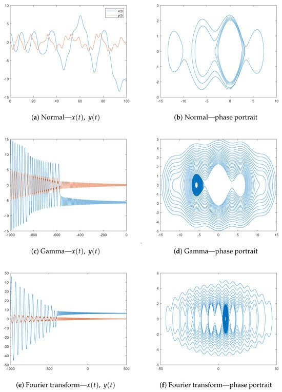
Figure 8.
Dynamics.
On the other hand, if we use a -gamma distribution, then its support is and the characteristic function is
Some simulations based on the values and are presented in Figure 8c,d. The other parameters are similar to those for Example 3—, , , . The initial condition is taken at and .
Under this construction, the underlying distribution drives the perturbations of the system via its characteristic function. Having in mind that it is the Fourier transform of the distribution’s density, we may influence the perturbations by an arbitrary function through its Fourier transform. Thus, if is the underlying function, then . For example, if the underlying function is for some p, then
Figure 8e,f present some simulations based on the parameters similar to ones used in Example 5, namely , , , and . The power p is stated at , whereas the initial condition is and .
Finally, let us discuss some limitations of the suggested approach for controlling the oscillations. First, Formula (9) is based on the characteristic functions of the probability distributions. The main criterion for to be a characteristic function is the Bochner’s theorem. Unfortunately, the condition for positive definiteness is often hard to verify. Some alternatives give the Mathias and Khinchine criteria. Additionally, Pólya’s theorem uses very simple conditions, but they are only sufficient.
On the other hand, nevertheless, we use Formula (9) based on the characteristic functions or the more general approach of the Fourier transform, the function may not exist in a closed form. Thus, some numerical alternatives have to be applied for approximation of —for example, Discrete Fourier Transform (DFT) or the Fast Fourier Transform (FFT).
4. Conclusions
In this article, we propose a new modified rf SQUID’s model. Several simulations are composed. We demonstrate also some specialized modules for investigating the dynamics of the proposed model. This will be included as an integral part of a planned much more general Web-based application for scientific computing. A number of authors devote their research on this topic to the case of ”strong damping” (see, for example, [9,12])
1. The reader can formulate and explore the dynamics of modified models of the type
using results obtained in the present paper. The case of highly damped systems is also of some interest and will be considered in future work.
The new model has many free parameters, which makes it attractive for engineering calculations, for example, for possible oscillation control—a user-preset level (or fork) for the oscillations of the y -component of the differential system solution.
The construction presented in Section 3.2 can be applied to Model (14) by using the exponential presentation of the sin-function
Thus dynamics (14) can be written as
We envisage future research on the current topic—modeling of chaotic systems (of the type (1) and (4)) with a desired set of properties—in the light of the interesting considerations in the articles [48,49].
Interesting results on the topic control of homoclinic chaos by weak periodic perturbations can be found in the monograph [50].
Other dynamic models from practice and their treatment in the light of the considerations in this paper.
2. The analytical study of controlling chaotic dynamics in spur gear systems is the subject of reflections by many authors working in the field of mechanisms and machine theory.
Gear systems have been widely used in many industrial applications due to their advantages of having accurate transmission ratios, compact dimensions, and high efficiency. With increasing requirements for gear performance in cutting-edge fields, many nonlinear dynamic characteristics that affect transmission performance must be considered in gear design.
Therefore, it is important to establish a relatively accurate dynamic model and investigate the complicated nonlinear behavior of the gear system subjected to various excitations. With the development of nonlinear dynamics theories, the nonlinear characteristics of these systems, such as stability, periodic responses, bifurcations, and chaos behaviors, have become the most interesting research areas.
A nonlinear dynamic model of a spur gear pair with backlash and static transmission error is formulated in [51].
More precisely, the conditions for existence of chaotic behavior in terms of homoclinic bifurcation by using Melnikov analysis are performed.
The planar model is of the form
where backlash function is a nonlinear displacement function and can be expressed as
where is a mechanical parameter. The authors in [51] consider the following approximation (for ): (see Figure 9) and study the dynamics of Model (17) using Melnikov analysis. Some investigations can be found in [52,53]. Dynamic response of a spur gear system with uncertain parameters is considered in [52]. Dynamic modeling and nonlinear analysis of a spur gear system considering a nonuniformly distributed meshing force is considered in [54].
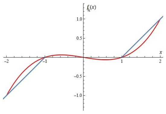
Figure 9.
Approximation of ( [51]).
The reader can formulate and explore the dynamics of modified model of the type
We will explicitly note that specialists working in the subject under consideration may also use other approximations of the backlash function .
For example, the following approximation can also be considered for (see Figure 10) and study the dynamics of Model (18) using considerations in this article.
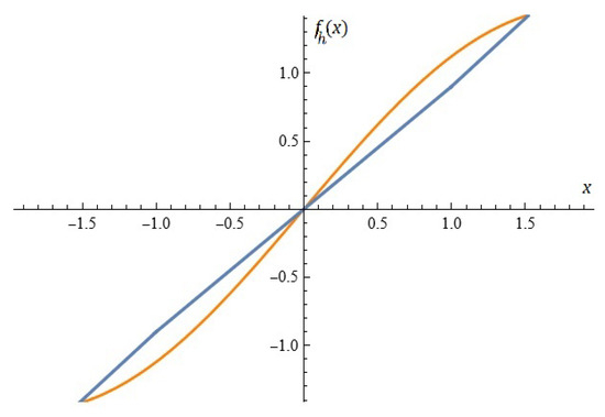
Figure 10.
A possible approximation of () by .
3. Following the considerations in this article, the reader can successfully formulate and investigate the dynamics of the following extended hypothetical oscillator
where , b is the damping level, is the damping exponent, and N is the integer.
At this stage, we will call Model (19) “hypothetical” until specialists and engineers working in this scientific field make a statement regarding its applicability.
Example 6.
Let us assume that the parameters and in (19) are fixed.
Let us further assume that the user has fixed the desired function
After applying an optimization technique, the desired control over the oscillations is achieved for the following values of the model parameters: , , , , , , , , , and (see Figure 11 and Figure 12).
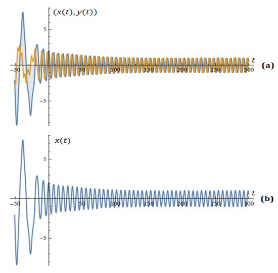
Figure 11.
(a) The solutions of the system (19); (b) component of solution (Example 6).
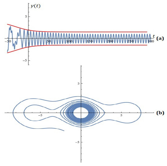
Figure 12.
(a) component of solution with restrictions; (b) phase space (Example 6).
Remark 1.
When more nonlinear damping terms are introduced, the following model is of interest to researchers:
Following the ideas given in [55], the reader can investigate the dynamics of the following extended hypothetical oscillator:
The task of generating a probabilistic construction with a view to possible control over the oscillations of the dynamic models (19) and (20) is also interesting. We envisage future research on this topic.
4. Regarding the practical implementation and control of oscillations, specialists and engineers working in this scientific field have the say.
5. We envisage future research on Melnikov analysis of chaotic dynamics in generalized oscillatory systems (based on (4), (14), (18), (19), and (20)) in light of the considerations in [55,56,57,58,59,60].
Author Contributions
Conceptualization, T.Z. and N.K.; methodology, N.K. and T.Z.; software, T.Z., T.B., N.K. and A.I.; validation, T.Z., A.I. and T.B.; formal analysis, N.K. and T.Z.; investigation, T.Z., N.K., T.B. and A.I.; resources, T.Z. and N.K.; data curation, T.B. and T.Z.; writing—original draft preparation, N.K. and T.Z.; writing—review and editing, T.B. and A.I.; visualization, T.B.; supervision, N.K. and T.Z.; project administration, T.Z.; funding acquisition, T.Z., T.B., N.K. and A.I. All authors have read and agreed to the published version of the manuscript.
Funding
The first and third authors are supported by the European Union-NextGenerationEU, through the National Plan for Recovery and Resilience of the Republic Bulgaria, project No BG-RRP-2.004-0001-C01. The research of the second and fourth authors was performed under the Project BG-RRP-2.011-0049 with the financial support by the European Union NextGenerationEU.
Data Availability Statement
Data are contained within the article.
Conflicts of Interest
The authors declare no conflicts of interest.
References
- Jaklevic, R.; Lambe, J.; Silver, A.; Mercereau, J. Quantum Interference Effects in Josephson Tunneling. Phys. Rev. Lett. 1964, 12, 159–160. [Google Scholar] [CrossRef]
- Clarke, J.; Braginski, A. (Eds.) The SQUID Handbook: Fundamentals and Technology of SQUIDs and SQUID Systems; Wiley-VCH: Weinheim, Germany, 2004. [Google Scholar]
- Clarke, J.; Braginski, A. (Eds.) The SQUID Handbook: Applications of SQUIDs and SQUID Systems; Wiley-VCH: Weinheim, Germany, 2006. [Google Scholar]
- Ritala, R.; Salomaa, M. Odd and even subharmonics and chaos in RF SQUIDS. J. Phys. C Solid State Phys. 1983, 16, 477–484. [Google Scholar] [CrossRef]
- Ritala, R.; Salomaa, M. Chaotic dynamics of periodically driven rf superconducting quantum interference devices. Phys. Rev. B 1984, 29, 6143–6154. [Google Scholar] [CrossRef]
- Fesser, K.; Bishop, A.; Kumar, P. Chaos in rf SQUID’s. Appl. Phys. Lett. 1983, 43, 123–124. [Google Scholar] [CrossRef]
- Schieve, W.; Bulsara, A.; Jacobs, E. Homoclinic chaos in the rf superconducting quantum-interference device. Phys. Rev. A 1988, 37, 3541–3552. [Google Scholar] [CrossRef]
- Ling, F.; Bao, G. A numerical implementations of Melnikov’s method. Phys. Lett. A 1987, 122, 413–417. [Google Scholar] [CrossRef]
- Salam, F. The Mel’nikov technique for highly dissipative systems. SIAM J. Appl. Math. 1987, 47, 232–243. [Google Scholar] [CrossRef]
- Schecter, S. Melnikov’s method at a saddle–node and the dynamics of the forced Josephson junction. SIAM J. Math. Anal. 1987, 18, 1699–1715. [Google Scholar] [CrossRef]
- Grebogi, C.; Ott, E.; Yorke, J. Basin boundary metamorphoses: Changes in accessible boundary orbits. Phys. 24 D 1987, 24, 243–262. [Google Scholar] [CrossRef]
- Bruhn, B.; Koch, B. Homoclinic and Heteroclinic Bifurcations in rf SQUIDs. Z. Naturforsch. 1988, 43a, 930–938. [Google Scholar] [CrossRef]
- Jackel, L.; Buhrman, R. Noise in the rf SQUID. J. Low Temp. Phys. 1975, 19, 201–246. [Google Scholar] [CrossRef]
- Ehnholm, G. Theory of the signal transfer and noise properties of the rf SQUID. J. Low Temp. Phys. 1977, 29, 1–27. [Google Scholar] [CrossRef]
- Likharev, K. Dynamics of Josephson Junctions and Circuits; Gordon Breach: New York, NY, USA, 1986. [Google Scholar]
- Ryhdnen, T.; Seppa, H.; Ilmoniemi, R.; Knuutila, J. SQUID magnetometers forlow-frequency applications. J. Low Temp. Phys. 1989, 76, 287–386. [Google Scholar] [CrossRef]
- Chesca, B. Theory of rf SQUIDs operating in the presence of large thermal fluctuations. J. Low Temp. Phys. 1998, 110, 963–1001. [Google Scholar] [CrossRef]
- Zeng, X.; Zhang, Y.; Chesca, B.; Barthel, K.; Greenberg, Y.; Braginski, A. Experimental study of amplitude-frequency characteristics of high-transition-temperature radio frequency superconducting quantum interference device. J. Appl. Phys. 2000, 88, 6781–6787. [Google Scholar] [CrossRef]
- Hansma, P. Superconducting single-junction interferometers with small critical currents. J. Appl. Phys. 1973, 44, 4191–4194. [Google Scholar] [CrossRef]
- Rifkin, R.; Vincent, D.; Deaver, B.; Hansma, P. Rf SQUIDs in the nonhysteretic mode: Detailed comparison of theory and experiment. J. Appl. Phys. 1976, 47, 2645–2650. [Google Scholar] [CrossRef]
- Kuzmin, L.; Likharev, K.; Migulin, V.; Polunin, E.; Simonov, N. X-band parametric amplifier and microwave SQUID using single-tunnel-junction superconducting interferometer. In SQUID’85, Superconducting Quantum Interference Devices and Their Applications; Hahlbohm, H.D., Lubbig, H., Eds.; Walter de Gruyter: Berlin, Germany, 1985; pp. 1029–1034. [Google Scholar]
- Zhang, Y. Evolution of HTS rf SQUIDs. IEEE Trans. Appl. Supercond. 2001, 11, 1038–1042. [Google Scholar] [CrossRef]
- Silver, A.; Zimmerman, J. Quantum states and transitions in weakly connected superconducting rings. Phys. Rev. 1967, 157, 317–341. [Google Scholar] [CrossRef]
- Giffard, R.; Webb, R.; Wheatly, J. Principles and methods of low frequency electric and magnetic measurements using an rf-biased point-contact superconducting device. J. Low Temp. Phys. 1972, 6, 533–611. [Google Scholar] [CrossRef]
- Buhrman, R. Noise limitations in rf SQUIDs. In Superconducting QuantumInterference Devices and Their Applications; Hahlbohm, H.D., Lubbig, H., Eds.; de Gruyter: Berlin, Germany, 1977; pp. 395–431. [Google Scholar]
- Buhrman, R.; Jackel, L. Performance factors in rf SQUIDs—High frequency limit. IEEE Tran. Magn. 1977, MAG-13, 879–882. [Google Scholar] [CrossRef]
- Keranen, R.; Kurkijarvi, J. Dependence on the pump frequency of the sensitivity of the rf SQUID. J. Low Temp. Phys. 1986, 65, 279–288. [Google Scholar] [CrossRef]
- Falko, C.; Parker, W. Operating characteristics of thin-film rf-biased SQUID’s. J. Appl. Phys. 1975, 46, 3238–3243. [Google Scholar] [CrossRef]
- Zhang, Y.; Muck, M.; Braginski, A.; Topfer, H. High-sensitivity microwave rf SQUID operating at 77 K. Supercond. Sci. Techn. 1994, 7, 269–272. [Google Scholar] [CrossRef][Green Version]
- Zhang, Y.; Muck, M.; Herrmann, K.; Schubert, J.; Zander, W.; Braginski, A.; Heiden, C. Sensitive rf SQUIDs and magnetometers operating at 77 K. IEEE Trans. Appl.Supercond. 1993, 3, 2465–2468. [Google Scholar] [CrossRef]
- Il’ichev, E.; Zakosarenko, V.; Ijsselsteijn, R.; Schultze, V. Inductive reply of high-Tc rf SQUID in the presence of large thermal fluctuations. J. Low Temp. Phys. 1997, 106, 503–508. [Google Scholar] [CrossRef]
- Chesca, B. On the theoretical study of an rf-SQUID operation taking into account the noise influence. J. Low Temp. Phys. 1994, 94, 515–538. [Google Scholar] [CrossRef]
- Greenberg, Y. Signal characteristics for high Tc rf SQUID from its small signal voltage-frequency characteristics. J. Low Temp. Phys. 1998, 114, 297–316. [Google Scholar] [CrossRef]
- Tan, J.; Zhang, K.; Li, B.; Wu, A. Event-Triggered Sliding Mode Control for Spacecraft Reorientation With Multiple Attitude Constraints. IEEE Trans. Aerosp. Electron. Syst. 2023, 59, 6031–6043. [Google Scholar] [CrossRef]
- Hou, X.; Xin, L.; Fu, Y.; Na, Z.; Gao, G.; Liu, Y.; Xu, Q.; Zhao, P.; Yan, G.; Su, Y.; et al. A self-powered biomimetic mouse whisker sensor (BMWS) aiming at terrestrial and space objects perception. Nano Energy 2023, 118, 109034. [Google Scholar] [CrossRef]
- Melnikov, V. On the stability of the center for time periodic perturbations. Trans. Mosc. Math. Soc. 1963, 12, 1–57. [Google Scholar]
- Golev, A.; Terzieva, T.; Iliev, A.; Rahnev, A.; Kyurkchiev, N. Simulation on a Generalized Oscillator Model: Web-Based Application. Comptes Rendus L’Academie Bulg. Des Sci. 2024, 77, 230–237. [Google Scholar] [CrossRef]
- Kyurkchiev, N.; Zaevski, T.; Iliev, A.; Kyurkchiev, V.; Rahnev, A. Generating Chaos in Dynamical Systems: Applications, Symmetry Results, and Stimulating Examples. Symmetry 2024, 16, 938. [Google Scholar] [CrossRef]
- Kyurkchiev, N.; Zaevski, T.; Iliev, A.; Branzov, T.; Kyurkchiev, V.; Rahnev, A. Dynamics of Some Perturbed Morse-Type Oscillators: Simulations and Applications. Mathematics 2024, 12, 3368. [Google Scholar] [CrossRef]
- Kyurkchiev, N.; Zaevski, T.; Iliev, A.; Kyurkchiev, V.; Rahnev, A. Modeling of Some Classes of Extended Oscillators: Simulations, Algorithms, Generating Chaos, Open Problems. Algorithms 2024, 17, 121. [Google Scholar] [CrossRef]
- Galchenko, M.; Fedoseev, P.; Andreev, V.; Kovacs, E.; Butusov, D. Semi-Implicit Numerical Integration of Boundary Value Problems. Mathematics 2024, 12, 3849. [Google Scholar] [CrossRef]
- Fedoseev, P.; Karimov, A.; Legat, V.; Butusov, D. Preference and stability regions for semi-implicit composition schemes. Mathematics 2022, 10, 4327. [Google Scholar] [CrossRef]
- Kareem, H.; Kovacs, E.; Janos, M.; Nagy, A.; Askar, A. Explicit Stable Finite Difference Methods for Diffusion-Reaction Type Equations. Mathematics 2021, 9, 3308. [Google Scholar] [CrossRef]
- Corless, R.; Essex, C.; Nerenberg, M. Numerical methods can suppress chaos. Phys. Lett. A 1991, 157, 27–36. [Google Scholar] [CrossRef]
- Ostrovskii, V.; Rybin, V.; Karimov, A.; Butusov, D. Inducing multistability in discrete chaotic systems using numerical integration with variable symmetry. Chaos Solitons Fractals 2022, 165, 112794. [Google Scholar] [CrossRef]
- Corless, R. Numerical methods for Chaotic ODE. arXiv 2025, arXiv:2501.06123. [Google Scholar]
- Kyurkchiev, N. Selected Topics in Mathematical Modeling: Some New Trends. Dedicated to Academician Blagovest Sendov (1932–2020); LAP LAMBERT Academic Publishing: Saarbrucken, Germany, 2020. [Google Scholar]
- Moysis, L.; Azar, A.; Kafetzis, I.; Tsiaousis, M.; Charalampidis, N. Introduction to control systems design using matlab. Int. J. Syst. Dyn. Appl. 2015, 6, 130–170. [Google Scholar] [CrossRef]
- Petavratzis, E.; Moysis, L.; Volos, C.; Stouboulos, I.; Nistazakis, H.; Valavanis, K. A chaotic path planning generator enhanced by a memory technique. Robot. Auton. Syst. 2021, 143, 103826. [Google Scholar] [CrossRef]
- Chacon, R. Control of homoclinic chaos by weak periodic perturbations. In World Scientific Series on Nonlinear Series; Chua, L., Ed.; World Scientific Publishing: Singapore, 2005; Volume 55. [Google Scholar]
- Saghafi, A.; Furshidianfer, A. The analytical study of controlling chaotic dynamics in spur gear systems. Mech. Mach. Theory 2016, 96, 179–191. [Google Scholar] [CrossRef]
- Guerine, A. Dynamic response of a spur gear system with uncertain parameters. J. Theor. Appl. Mech. 2016, 54, 1039–1049. [Google Scholar] [CrossRef]
- Dalpiaz, G.; Rivola, A.; Rubini, R. Dynamic modeling of gear systems for condition monitoring and diagnostics. In Proceedings of the Congress on Technical Diagnostics, Gdansk, Poland, 17–20 September 1996; pp. 185–192. [Google Scholar]
- Jin, B.; Bian, Y.; Liu, X.; Gao, Z. Dynamic Modeling and Nonlinear Analysis of a Spur Gear System Considering a Nonuniformly Distributed Meshing Force. Appl. Sci. 2022, 12, 12270. [Google Scholar] [CrossRef]
- Zhou, Y.; Zhao, P.; Guo, Y. Melnikov analysis of chaotic dynamics in an impact oscillator system. Int. J. Non-Linear Mech. 2025, 171, 105027. [Google Scholar] [CrossRef]
- Liu, D.; Xu, Y. Random Disordered Periodical Input Induced Chaos in Discontinuous Systems. Int. J. Bifurc. Chaos 2019, 29, 1950002. [Google Scholar] [CrossRef]
- Li, Y.; Wei, Z.; Zhang, W.; Yi, M. Melnikov-type method for a class of hybrid piecewise-smooth systems with impulsive effect and noise excitation: Homoclinic orbits. Chaos 2022, 32, 073119. [Google Scholar] [CrossRef] [PubMed]
- Tian, R.; Zhou, Y.; Wang, Y.; Feng, W.; Yang, X. Chaotic threshold for non-smooth system with multiple impulse effect. Nonlinear Dynam. 2016, 85, 1849–1863. [Google Scholar] [CrossRef]
- Guo, X.; Tian, R.; Xue, Q.; Zhang, X. Sub-harmonic melnikov function for a high dimensional non-smooth coupled system. Chaos Solitons Fractals 2022, 164, 112629. [Google Scholar] [CrossRef]
- Zheng, Y.; Zhang, W.; Liu, T.; Zhang, Y. Resonant responses and double-parameter multi-pulse chaotic vibrations of graphene platelets reinforced functionally graded rotating composite blade. Chaos Solitons Fractals 2022, 156, 111855. [Google Scholar] [CrossRef]


Disclaimer/Publisher’s Note: The statements, opinions and data contained in all publications are solely those of the individual author(s) and contributor(s) and not of MDPI and/or the editor(s). MDPI and/or the editor(s) disclaim responsibility for any injury to people or property resulting from any ideas, methods, instructions or products referred to in the content. |
© 2025 by the authors. Licensee MDPI, Basel, Switzerland. This article is an open access article distributed under the terms and conditions of the Creative Commons Attribution (CC BY) license (https://creativecommons.org/licenses/by/4.0/).