Article

A Self-Normalized Online Monitoring Method Based on the Characteristic Function

Department of Statistics, School of Mathematics, Southwest Jiaotong University, Chengdu 611756, China
*
Author to whom correspondence should be addressed.
Mathematics 2025, 13(5), 710; https://doi.org/10.3390/math13050710
Submission received: 6 December 2024 / Revised: 9 February 2025 / Accepted: 18 February 2025 / Published: 22 February 2025

Abstract

:
The goal of nonparametric online monitoring methods is to quickly detect structural changes in the distribution of a data stream. This work is concerned with a nonparametric self-normalized monitoring method based on the difference of empirical characteristic functions. This method introduces an additional self-normalization factor, which enables effective control the Type I error. We theoretically investigate the asymptotic properties of the monitoring method under the null hypothesis as well as the alternative hypothesis. Since the asymptotic distribution under the null hypothesis is quite complicated, we apply the multivariate stationary bootstrap method to estimate the critical value of the sequential test. Numerical simulations and a real-world application demonstrate the usefulness of the proposed method.

1. Introduction

Since the seminal work of Page [1], the change point problem has attracted significant attention. Change point detection methods aim to identify structural changes in the statistical properties (e.g., mean, variance, and probability distribution function) of a time series, or in the parameters of a statistical model. Traditionally, change point detection methods are classified into two types: offline change point detection (retrospective tests) and online monitoring (sequential tests). Offline methods are designed to detect structural changes in a given historical dataset, with several reviews available [2,3]. In contrast, online monitoring methods focus on rapidly detecting structural changes in real-time data streams, addressing the change point monitoring problem [4]. Online monitoring methods are widely applied in fields such as quality control, environmental protection, medical monitoring, and structural health monitoring.
For change point monitoring, the Cumulative Sum (CUSUM) method is a commonly used tool for detecting structural breaks [5]. Many CUSUM monitoring schemes have been proposed to quickly detect structural breaks in the mean, variance, regression coefficients, etc. For instance, Horváth et al. [6] proposed two CUSUM monitoring schemes based on residuals and recursive residuals for detecting change in regression coefficients of linear models. The CUSUM method for detecting mean shifts is discussed by Aue et al. [7] and for identifying structural changes in variance can be found in Horváth et al. [8]. Berkes et al. [9] proposed a CUSUM statistic based on the quasi-likelihood score function to quickly detect parameter changes in GARCH models. Na et al. [10] explored online monitoring schemes for monitoring various parameters in time series models. Based on the estimating functions, Kirch and Kamgaing [11] studied the change point monitoring problem of parameters in general time series models. Gösman et al. [12] investigated the change point monitoring problem for the mean of high-dimensional time series.
For time series data collected over a long period, making parametric model assumptions about the data is often unrealistic. Misspecified parametric models may result in an unreliable online monitoring scheme [13]. Furthermore, if we assume that a structural change occurs in one statistical characteristic (e.g., mean) while it actually occurs in another (e.g., variance), the CUSUM methods designed to monitor a specific parameter may lead to misleading conclusions [14]. In contrast, the nonparametric online monitoring methods designed to detect structural changes in the probability distribution of the observations are more robust [15], because these methods do not require modeling the data or assigning a specific type of change point in advance. A review of early nonparametric online monitoring methods can be found in [16]. Building upon these previous approaches, Hlávka et al. [17] proposed a CUSUM statistic based on the empirical characteristic function for rapidly detecting structural change in the distribution function of paired multivariate time series. To address the changing point monitoring problem for a distribution function of multivariate time series, Kojadinovic and Verdier [18] proposed a CUSUM monitoring scheme based on the empirical distribution function. Expanding on the concept of stationarity testing [19], Lee et al. [20] introduced a CUSUM statistic based on the joint characteristic function, which is designed to detect structural breaks in the stationarity of univariate time series. Some recently proposed nonparametric online monitoring methods in different contexts can be found in [21,22].
However, both the parametric and nonparametric CUSUM methods discussed above are subject to the problem of empirical size distortion. For example, in CUSUM methods designed to monitor a specific parameter, estimating the long run variance (LRV) poses a challenge. The commonly used kernel-based LRV estimators are sensitive to the bandwidth parameter, making it difficult to select an appropriate value in practice [23]. Thus, parametric CUSUM methods that directly estimate the LRV may suffer from empirical size distortion, particularly when the sample size is small and the model is difficult to estimate [9,10]. To overcome this drawback, Shao and Zhang [23] introduced a self-normalization factor to avoid directly estimating the LRV. This approach led to the development of the self-normalized CUSUM statistic, which effectively controls the Type I error. Despite its effectiveness, there are relatively few studies on self-normalized CUSUM methods in change point monitoring. For instance, Hoga [24] introduced a ratio type (self-normalized) CUSUM statistic for monitoring the mean of multivariate time series. Dette and Gösman [25] proposed a self-normalized CUSUM statistic based on the maximum likelihood ratio for detecting structural changes in a general class of parameters. Chan et al. [26] proposed a self-normalized CUSUM statistic based on the generalized objective function, which was designed to quickly detect structural changes in the parameters of general time series models.
When the sample size is small and there is a strong temporal dependence between observations, the empirical size of existing nonparametric online monitoring methods becomes severely distorted, as shown in the simulation results in [17,18,20]. To the best of our knowledge, the concept of self-normalization has not yet been considered in studies of nonparametric online monitoring methods. To fill this gap, drawing on the ideas of Chan et al. [26], we propose a self-normalized CUSUM statistic based on the empirical characteristic function, which is designed to quickly detect distributional changes in multivariate time series. We theoretically studied the asymptotic properties of the monitoring statistic under the null hypothesis as well as the alternative hypothesis. Since the asymptotic distribution under the null hypothesis is quite complicated, we use the multivariate stationary bootstrap method to estimate the critical value of the sequential test. Numerical simulations demonstrate that our method can control the empirical size effectively. Finally, we apply the proposed method to vibration data from wind turbine blades, illustrating its practical utility in real-world scenarios.

2. Self-Normalized Monitoring Method

Let { X t } , t = 1 , be a d-dimensional time series with probability distribution function F t ( u ) = Pr ( X t u ) , u R d . The change point monitoring problem for the distribution function is outlined as follows. Prior to the start of monitoring, we assume that a stationary historical dataset { X 1 , , X m } has been collected, which satisfies F 1 = = F m . These existing observations are referred to as the training sample. Subsequently, new observations X m + 1 , X m + 2 , arrive one by one. The online monitoring method will continuously detect structural changes in the distribution function of the data stream, testing the following hypothesis at each step:
H 0 : F t = F m , t = m + 1 , , m + L m , H 1 : F t = F m , m + 1 t m + k * ; F t F m , m + k * + 1 t m + L m ,
where F m , F t are the unknown distribution functions, m + k * denotes the unknown change point, and L represents the monitoring period specified by the user. The null hypothesis can be equivalently stated as
H 0 : ϕ t = ϕ m , t = m + 1 , , m + L m ,
where ϕ t = E ( e i u , X t ) is the characteristic function of random vector X t , i = 1 and x , y denotes the inner product of vectors.
At each new observation X m + k , 1 k L m arrival, we are interested in finding a quantity (referred to as the detector) that captures the difference in distribution between the training sample and the newly arrived sample. To this end, we will compare an estimator of the characteristic function ϕ X t , t { m + 1 , , m + k } with the corresponding estimator derived from the observations prior to time m. Considering the superior performance of self-normalization methods in controlling Type I errors, and drawing inspiration from Chan et al. [26], we propose the following detector statistic:
Γ m S N ( k ) = Γ m ( k ) S m 2 , k = 1 , , L m ,
where
Γ m ( k ) = ( m + k ) 2 m R d ϕ ^ 1 : m ( u ) ϕ ^ 1 : m + k ( u ) 2 ω ( u ) d u = 1 m R d t = m + 1 m + k e i X t , u k m t = 1 m e i X t , u 2 ω ( u ) d u ,
S m 2 = 1 m 2 t = 1 m R d t 2 | ϕ ^ 1 : t ( u ) ϕ ^ 1 : m ( u ) | 2 ω ( u ) d u ,
where k denotes the sample size of the newly arrived samples after monitoring begins, and ϕ ^ a : b ( u ) = 1 b a + 1 t = a b e i X t , u is the empirical characteristic function based on the samples { X a , , X b } . Γ m ( k ) is the CUSUM-type detector statistic introduced by Lee et al. [20] and S m 2 is the self-normalization factor that we introduced. ω ( u ) is a suitable weight function that ensures the existence of the integral in Equations (4) and (5). If ω ( u ) is a non-negative symmetric function, then we obtain
Γ m ( k ) = ( m + k ) 2 m 1 m 2 μ , ν = 1 m H μ , ν + 1 ( m + k ) 2 μ , ν = 1 m + k H μ , ν 2 m ( m + k ) μ = 1 m ν = 1 m + k H μ , ν , S m 2 = 1 m 2 t = 1 m t 2 1 m 2 μ , ν = 1 m H μ , ν + 1 t 2 μ , ν = 1 t H μ , ν 2 m t μ = 1 m ν = 1 t H μ , ν ,
where H μ , ν = H ( X μ X ν ) and H ( x ) = R d cos x , u ω ( u ) d u . Following Hlávka et al. [17], we choose the weight function ω ( u ) = exp { a u 2 } , where a > 0 is a tuning parameter. Then, the direct calculation gives H ( x ) = ( π a ) d / 2 exp { x 2 4 a } . Generally, the choice of the weight function ω ( · ) is typically based on considerations of computational convenience, as discussed in [17]. There are several options for the weight function that can turn H ( x ) into a closed-form expression, as shown in Fan et al. [27]. One might wonder how the choice of weight function affects the performance of the resulting test, or whether there exists a weight function that is optimal in some sense. As pointed out by Lee et al. [20], this issue is extremely non-trivial. We will examine the impact of different options of weight function through simulation, with results provided in the Sections S2.1 and S2.2 of the Supplementary Materials. If the distribution function of { X t } changes after a certain time m + k * , the value of Γ m S N ( k ) will be very large for k > k * . Then, we reject the null hypothesis if the detector Γ m S N ( k ) is ‘too large’. For each newly arrived observation X m + k , what value of Γ m S N ( k ) is considered ‘too large’ is specified by a boundary function q ( k m ) , which usually increases monotonically with k; see [4,11]. Namely, the null hypothesis will be rejected at the first time point, denoted by k, for which it holds:
D m S N ( k ) = Δ 1 q 2 ( k m ) Γ m S N ( k ) > C α ,
where C α is the critical value that can be obtained by the limit distribution of the statistic max 1 k L m D m S N ( k ) under the null hypothesis. Equivalently, an alarm is given as soon as the detector statistic Γ m S N ( k ) first exceeds the critical curve given by C α q k m 2 . The function q · is a suitable so-called boundary function used to control the asymptotic global Type I error of the online monitoring method; see [20,28]. Following Chan et al. [26], we choose the boundary function as q ( θ ) = ( 1 + θ ) , θ > 0 . Here, we refer to D m S N ( k ) as the self-normalized monitoring statistic, and for comparison, we take D m ( k ) = Δ 1 q 2 ( k m ) Γ m ( k ) to be the monitoring statistic without introducing the self-normalization factor.
The test procedure for testing the hypothesis H 0 against H 1 in our sequential setup is described using the stopping time τ ( m ) , which is defined as follows:
τ ( m ) = inf k : D m S N ( k ) > C α , 1 k L m , , if D m S N ( k ) C α , for all 1 k L m ,
where the constant C α is the critical value of the sequential test. The stopping time τ ( m ) indicates the time point at which monitoring ends. The online monitoring method follows the stopping rule described below. Monitoring stops when either the self-normalized monitoring statistic exceeds the critical value C α , or the number of collected observations reaches the predetermined amount L m . In other words, starting from k = 1 , we check successively whether the condition D m S N ( k ) > C α holds. If this condition is met, we set τ ( m ) = k and reject the null hypothesis. Otherwise, we continue to wait for a new observation and checks the condition D m S N ( k + 1 ) > C α once again. Specifically, if the null hypothesis is never rejected throughout the entire monitoring period, we stop monitoring.

3. Asymptotic Properties

Firstly, we investate the asymptotic distribution of the monitoring statistic under the null hypothesis, with the imposition of certain assumptions following Hlávka et al. [17].
Assumption 1. 
Suppose { X t } is a d-dimensional strictly stationary strong mixing sequence with mixing coefficients α ( h ) . For some constants κ > 0 and δ > 0 , there exists a constant C such that h = 0 ( h + 1 ) κ 2 α ( h ) δ 2 + κ + δ C . In addition, we assume that E X t 2 + κ + δ < .
Assumption 2. 
ω ( u ) is a non-negative symmetric integrable function, R d u 4 ω ( u ) d u < .
The mixing condition in Assumption 1 limits the temporal dependence of { X t } . Generally, the mixing coefficients are defined to quantify the strength of dependence between two segments of a time series that are separated by time. For a time series { X t } and h N , define the α -mixing coefficient α ( h ) = sup A F 0 , B F h P A B P ( A ) P ( B ) , where F a b denotes the σ -field generated by { X t ; a t b } . If α ( h ) 0 as h , then the process { X t } is said to be strong mixing. Assumption 2 imposes mild conditions on the weight function ω ( u ) , ensuring the existence of the integral in Equations (4) and (5). Some probability density functions of symmetric distribution with finite fourth moments satisfy this assumption and can be used as the weight function. The asymptotic distribution of the monitoring statistic under the null hypothesis is as follows.
Theorem 1. 
Suppose that Assumptions 1 and 2 hold, then under the null hypothesis as m the limit distribution of
max 1 k L m D m S N ( k )
is the same as
sup θ ( 0 , L ) 1 ( 1 + θ ) 2 R d Z 1 ( θ , u ) θ Z 2 ( 1 , u ) 2 ω ( u ) d u 0 1 R d Z ( θ , u ) θ Z ( 1 , u ) 2 ω ( u ) d u d θ
where { Z ( θ , u ) } is a centered Gaussian process with covariance structure
cov { Z ( θ 1 , u 1 ) , Z ( θ 2 , u 2 ) } = θ 1 θ 2 Σ ( u 1 , u 2 ) ,
where Σ ( u 1 , u 2 ) = j = 0 cov h 1 ( u 1 ) , h 1 + j ( u 2 ) + j = 1 cov h 1 ( u 2 ) , h 1 + j ( u 1 ) and θ 1 θ 2 = min ( θ 1 , θ 2 ) , h t ( u ) = cos X t , u + sin X t , u .   Z 1 ( θ , u ) and Z 2 ( θ , u ) are two independent centered Gaussian processes with similar covariance structure.
Theorem 1 provides the asymptotic distribution of the monitoring statistic under the null hypothesis, which helps to determine the critical value C α ensuring that the monitoring scheme has asymptotic size α :
lim m Pr ( τ ( m ) < H 0 ) = Pr sup θ ( 0 , L ) 1 ( 1 + θ ) 2 R d Z 1 ( θ , u ) θ Z 2 ( 1 , u ) 2 ω ( u ) d u 0 1 R d Z ( θ , u ) θ Z ( 1 , u ) 2 ω ( u ) d u d θ > C α = α .
The above asymptotic results in Theorem 1 are derived based on our default choice of boundary function q ( θ ) = ( 1 + θ ) , θ > 0 . The selection of the boundary function has been investigated by several authors (see [4,11,25,28,29,30]) and we will compare different options through simulation presented in the Section S2.3 of the Supplementary Materials. As noted by Dette and Gösman [25], one can choose a suitable function (which is increasing and bounded from below by a positive constant, or which satisfies some other regularity condition as shown in [29]) and then specify the constant C α as the corresponding quantile of the asymptotic distribution to ensure that the monitoring scheme has asymptotic size α .
Next, we derive the asymptotic results under the alternative hypothesis.
Assumption 3. 
Suppose k * = m θ * , θ * ( 0 , L ) is the change point, where x is the largest integer less than or equal to x. Let ϕ t be the characteristic function of X t , then we can assume that
ϕ t = ϕ ( 0 ) , t = 1 , , m + k * , ϕ ( ) , t = m + k * + 1 , , L m .
where ϕ ( 0 ) and ϕ ( ) refer to the characteristic functions before and after the change point.
Theorem 2. 
Suppose that Assumptions 2 and 3 are true, then under the alternative hypothesis
max 1 k L m D m S N ( k ) Pr , m .
Theorem 2 shows the consistency of the proposed online monitoring method under the alternative hypothesis. When the distribution function of { X t } undergoes a structural change, the method achieves asymptotic power 1, lim m Pr ( τ ( m ) < H 1 ) = 1 .
As shown in Theorem 1, the asymptotic distribution of the proposed nonparametric self-normalized CUSUM monitoring statistic is quite complicated. It is not easy to determine the critical value C α by the asymptotic distribution. Therefore, we employ the multivariate stationary bootstrap method [31] to estimate the critical value of the sequential test. Let { U j } and { l j } be independent random variables, where U j follows a discrete uniform distribution on { 1 , , m } and l j follows the geometric distribution with parameter p b . Define R U j , l j as a random block starting at X U j with block length l j , i.e., R U j , l j = { X U j , , X U j + l j 1 } . The block length parameter p b represents the average length of the random block R U j , l j .
The stationary bootstrap method generates pseudo-samples by extracting random blocks from the training sample. For univariate time series ( d = 1 ), Politis and White [32] proposed an adaptive algorithm for selecting the block length parameter p b . For multivariate time series ( d > 1 ), we extend this algorithm to each component of the series, as suggested by Jentsch and Rao [33]. Then, we use the harmonic mean of the obtained block length parameters { p b 1 , , p b d } as the overall block length parameter, i.e, p b = d 1 p b 1 + + 1 p b d . The specific steps of the multivariate stationary bootstrap algorithm are as follows:
Step 1
Connect the training samples { X 1 , , X m } by their time index numbers to form a ring.
Step 2
Draw a series of random blocks R U j , l j for j = 1 , , n from the ring formed by the training sample, where n = min K , j = 1 K l j m + L m . Merge these blocks sequentially and select the first m + L m observations as the pseudo-sample, denoted as X 1 * , , X m + L m * .
Step 3
Treat the first m bootstrap observations as training sample { X 1 * , , X m * } and compute the bootstrap statistic: D * = max 1 k L m D m S N ( k ) .
Step 4
Repeat step 2 and 3 for a total of B times to get B bootstrap statistics. Sort these statistics in ascending order as D 1 * , , D B * . Then, the critical value is estimated as C α = D B ( 1 α ) * .
We followed the choices and suggestions of Lee et al. [20] and Jentsch and Rao [33] in employing the stationary bootstrap method. However, proving the consistency of the stationary bootstrap with certain adjustments in our context is temporarily beyond the scope of our work, though we are actively working on further investigating this property. Concerning the consistency of the stationary bootstrap, Lee et al. [20] provide a rigorous proof within their framework. Furthermore, Weber [29] offers a thorough proof of the consistency of the widely used block bootstrap method. The validity of the bootstrap method we employed is verified through simulation studies presented in Section 4. These results indicate that the proposed method performs well in practice, despite the ongoing investigation of its consistency.

4. Numerical Simulation

In this section, we investigate the finite sample performance of the proposed online monitoring method using numerical simulations. All empirical results are based on 1000 replications and sequential tests are conducted at the 5% significance level. The training sample sizes are m = { 100 , 200 } and the monitoring periods are L = { 1 , 2 , 3 } . First, we compare D m S N with the corresponding monitoring statistic that does not include the self-normalization factor, denoted as D m = Δ 1 q 2 ( k m ) Γ m ( k ) . For the monitoring statistics D m and D m S N , the parameter in the weight function ω ( u ) is set to a = 1 . Since the simulation of these two characteristic-function-based monitoring schemes is very time consuming, we followed Lee et al. [20] to conduct simulation experiments using the wrap-speed method [34]. We also compare the proposed method with two other online monitoring methods based on the empirical distribution function. Following the notation of Kojadinovic and Verdier [18], these comparison methods are denoted as Q m , k and T m , q . Specifically, Q m , k is the standard CUSUM-type statistic based on the empirical distribution function, while T m , q is a modified CUSUM-type statistic, as detailed in [18]. We focused on comparing the size, power, and average detection delay (that is, the delay between the first alarm and the actual change point) of all monitoring schemes.
In addition, for our monitoring scheme, different choices of the weight function ω ( u ) and the boundary function q ( θ ) may affect the performance of the monitoring procedures. For this reason, we provide some additional simulation results in the Supplementary Materials to investigate more deeply how different choices of these two functions affect the performance of the proposed method.

4.1. Under the Null Hypothesis

In this section, we investigate the performance of the proposed online monitoring method under the null hypothesis. Throughout, 0 denotes a two-dimensional zero vector and I 2 denotes the 2 × 2 identity matrix. Furthermore, ϵ t i . i . d . N 0 , I 2 unless otherwise stated. Following the setting of Kojadinovic and Verdier [18], we generated a series of bivariate AR(1) models with different regression coefficients, given by X t = β I 2 X t 1 + ϵ t , where β { 0 , 0.3 , 0.5 , 0.7 , 0.9 , 0.3 , 0.5 , 0.7 , 0.9 } . We denote these models as N 1 to N 9 . Additionally, we introduce two vector autoregressive models with weak and strong temporal dependence, labeled as N 10 and N 11 , respectively. Lastly, the BEKK-GARCH(1,1) model, denoted as N 12 , is adapted from the work of Hlávka et al. [17].
( N 10 )
X t = A X t 1 + ϵ t , where A = 0.1 0.05 0.05 0.1 .
( N 11 )
X t = A X t 1 + ϵ t , where A = 0.5 0.2 0.2 0.1 .
( N 12 )
BEKK-GARCH(1,1) model
X t = H t 1 2 ϵ t , ϵ t N ( 0 , I 2 ) , H t = C C + A X t 1 X t 1 A + B H t 1 B ,
where C = 10 3 4 5 0 3 , A = 0.254 0.004 0.04 0.332 , B = 0.941 0.023 0.019 0.864 .
Table 1 presents the empirical size for all online monitoring methods. Progressing from models N 1 to N 5 , with β ranging from 0 to 0.9, the temporal dependence between observations increases step by step. In the case of independent observations ( N 1 with β = 0 ), the empirical sizes of Q m , k , T m , q , and D m are close to the nominal levels. However, as temporal dependence increases, the empirical sizes of these three methods become significantly distorted. In contrast, the empirical size of the self-normalized method D m S N remains close to the nominal level across all five models ( N 1 N 5 ). When β is negative (models N 6 N 9 , with β ranging from −0.3 to −0.9), it appears that the impact of the temporal dependence on the empirical size is less obvious than when β is positive. But when the absolute value of β is larger ( N 8 with β = 0.7 and N 9 with β = 0.9 ), only the self-normalized method D m S N performs well. For models N 10 and N 11 , D m S N also performs well, while the empirical size of the other three online monitoring methods are distorted. In the BEKK-GARCH(1,1) model N 12 , the empirical sizes of the methods based on the empirical distribution function ( Q m , k and T m , q ) are severely distorted, while the methods based on the empirical characteristic function ( D m and D m S N ) perform better. Overall, the self-normalized online monitoring method D m S N effectively controls the Type I error regardless of the strength of temporal dependence.

4.2. Under the Alternative Hypothesis

In some models under the null hypothesis, we introduced structural changes in mean or variance to evaluate the performance of the proposed online monitoring methods under the alternative hypothesis. The change point is located at m + k * , 1 < k * < L m and δ represents the magnitude of change. The following models are considered:
Mean change
(M1)
X t = ϵ t + δ μ 1 I { t > m + k * } , where μ 1 = ( 1 , 1 ) .
(M2)
X t = A X t 1 + ϵ t + δ μ 1 I { t > m + k * } , where A = 0.1 0.05 0.05 0.1 , μ 1 = ( 1 , 1 ) .
(M3)
As in M 2 except that A = 0.5 0.2 0.2 0.1 .
Variance Change
(V1)
X t = ϵ t , ϵ t = η t I { t m + k * } + η t * I { t > m + k * } and η t N ( 0 , I 2 ) , η t * N ( 0 , ( 1 + δ ) I 2 ) .
(V2)
X t = A X t 1 + ϵ t , where A = 0.1 0.05 0.05 0.1 and ϵ t is the same as in V 1 .
(V3)
As in V 2 except that A = 0.5 0.2 0.2 0.1 .
(V4)
Let X t denote the BEKK-GARCH (1,1) model as in model N 12 and assume its variance changes in such a way that ϵ t = η t I { t m + k * } + η t * I { t > m + k * } and η t N ( 0 , I 2 ) , η t * N 0 , ( 1 + δ ) I 2 .
For the mean change models (M1)–(M3), the temporal dependence between observations gradually increases, while their mean vectors shift from 0 to δ μ 1 after time m + k * . For the variance change models (V1)–(V4), the variances in the error term components increase from 1 to 1 + δ .
First, we compared the power and average detection delays of all online monitoring methods across different magnitudes of change. We set m = 100 , L = 1 , and the change occurs at observation m + k * = 120 . The detection delay is calculated as τ ( m ) 120 . Following Dette and Gösman [25], simulation runs without rejection or those where rejection occurs before the actual change are excluded.
The left column in Figure 1 shows the empirical power of all monitoring schemes, while the right column displays the corresponding mean detection delays. When the variance changes, the empirical characteristic-function-based methods ( D m , D m S N ) significantly outperforms the comparison methods ( Q m , k , T m , q ) in both power and detection delay. For models with strong temporal dependence ( M 3 and V 3 ), only the self normalized method D m S N effectively controls the test size. Overall, the characteristic-function-based methods outperform those based on the distribution function in terms of mean detection delay and show comparable performance.
Next, we will compare the overall detection capabilities of the proposed method with those of the comparison methods for change points at different positions. For each model, given the magnitude δ , and following the setup in [20], we set the random change point as m + k * = m ( 1 + L U ) , where U follows a uniform distribution on the interval ( 0 , 0.8 ) .
Table 2 shows the overall empirical power of the sequential tests. For models (M1)–(M3), the power of all methods decreases as temporal dependence between observations increases. Dette and Gösmann [25] pointed out that stronger temporal dependence leads to a larger long run variance, making it difficult to separate structural changes in the mean from random noise. In models (M1) and (M2), where the mean undergoes a structural change and the temporal dependence is relatively weak, the empirical power of all online monitoring methods is quite close. In the model (M3), the empirical power of the self-normalized online monitoring method D m S N is lower compared to D m . As the sample size increases, the difference in empirical power between this two methods gradually decreases. For the models of change in variance (V1)–(V3), the monitoring methods based on the empirical characteristic function ( D m and D m S N ) significantly outperform the methods based on the empirical distribution function ( Q m , k and T m , q ). In the model (V4), Q m , k and T m , q have higher empirical power. However, when applied to the multivariate GARCH model N 12 , Q m , k and T m , q suffer from significant size distortion, while D m and D m S N turn out to be more reliable. Overall, the proposed self-normalized online monitoring method D m S N significantly improves the distorsion of the empirical size and shows good test power.

5. Data Example

The vibration signal of the wind turbine blades reflects the state of blades. Condition monitoring of the blades is crucial for the operation and maintenance of the wind turbine. The data used in this study were collected from wind turbines #1 and #5 at a wind farm in China. The vibration signals of three blades were collected by vibration sensors (installed in the same position) inside the blades. The sampling frequency of the signal acquisition system is 2560 Hz, the acquisition interval is 2 h, and the number of samples collected each batch is 128 KB. Data collection began at 10:00 on 21 September 2023, and continued with batches sent back every 2 h. A total of 134 and 99 valid vibration data batches were collected from wind turbine #1 and wind turbine #5, respectively.
As each batch of vibration signals arrives, the signals of three blades are first processed using a 10th-order high-pass Butterworth filter with a 0.1 Hz cutoff frequency. Then, features related to the vibration state of the blades are extracted from each batch of pre-processed signals. Each batch is divided into 8 time periods, and the root mean square (RMS) of the vibration signals for each blade in each short period is calculated: { R M S t 1 , R M S t 2 , R M S t 3 } . The RMS represents the vibration strength of the blades. For a signal { U 1 , , U N } of length N, the RMS is calculated as R M S = 1 N j = 1 N U j 2 . Under normal operating conditions, the vibration strength of three blades are close to each other. Based on this property, we calculate the difference between two consecutive RMSs of three blades to obtain the following monitoring indicator:
X t = X t 1 X t 2 X t 3 = R M S t 1 R M S t 2 R M S t 2 R M S t 3 R M S t 3 R M S t 1 , t = 1 , .

5.1. Wind Turbine #1

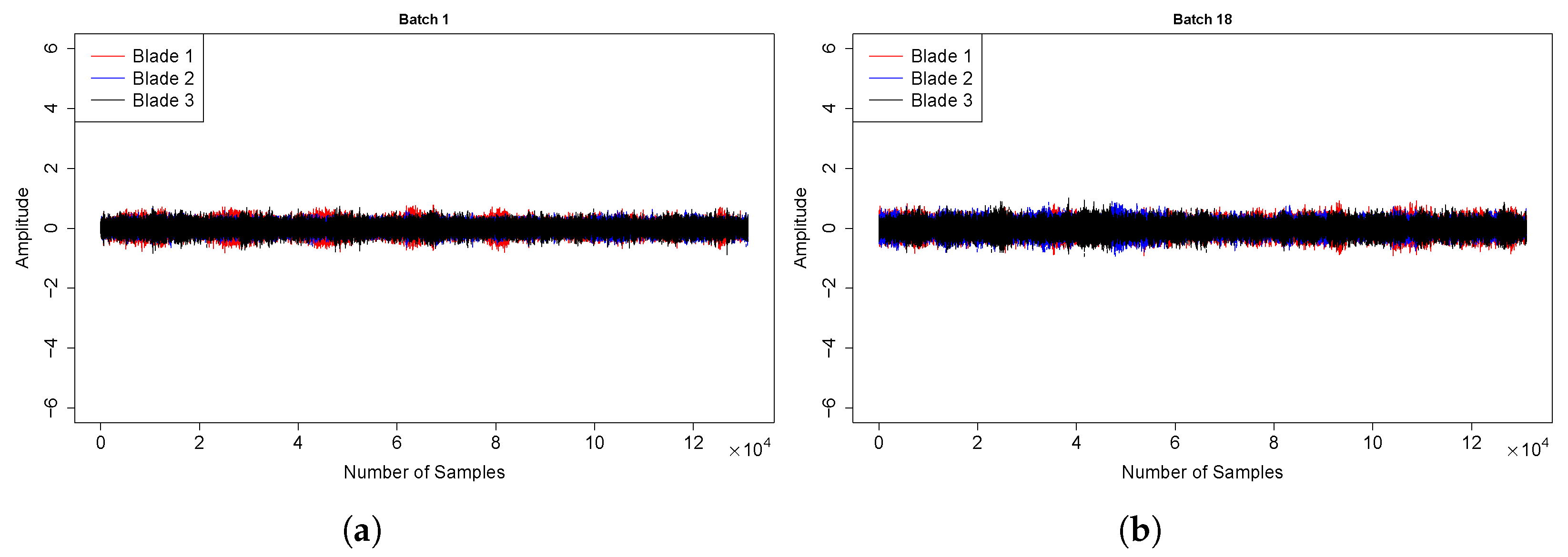
For wind turbine #1, we extracted the monitoring indicators { X t } , t = 1 , , 144 from the vibration signals in the first 36 h (18 batches) and used these data as the training sample. As mentioned earlier, under normal operating conditions, the vibration strength of the three blades should be similar to each other. As shown in Figure 2a,b, the vibration amplitudes of the three blades during the training phase are very close, indicating that the blades are in overall good condition.
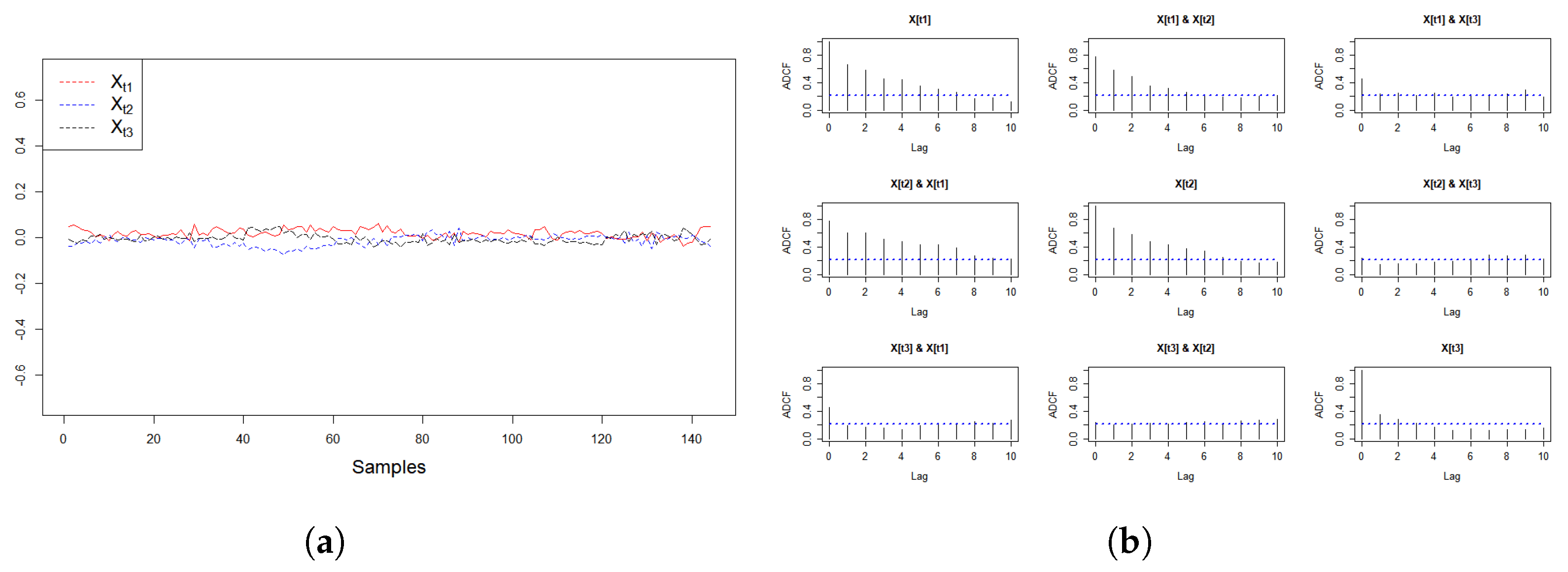
Before monitoring begins, we conduct some necessary analysis during the training phase, including temporal dependence analysis and testing the stationarity of the training sample. As illustrated in Figure 3a, the training sample appear to be stationary and free of change point. We applied the functions cpDist() of the R package npcp (version 0.2-6) [35] and e.divisive() of the R package ecp (version 3.1.6) [36] to detect changes in the training sample. The test results show that, under the significance level α = 5 % , there is no significant change in the distribution of the training sample. This also confirms the preliminary observation in Figure 2, where the vibration strengths of the three blades were similar during the training phase. In addition, we used the Auto Distance Correlation Function (ADCF) [37] to analyze the temporal dependence of the training sample. According to Figure 3b, the training samples exhibit strong temporal dependence. The components of the monitoring indicator X t are strongly correlated, and each component shows a significant temporal dependence. This is expected as the three blades form an interconnected system and their vibration modes are closely related. Moreover, the vibration state of the blades in subsequent periods is influenced by the vibrations in previous periods, thus leading to a significant temporal dependence.
To avoid a high Type I error, we use the proposed self-normalized online monitoring method D m S N to monitor the indicator { X t } . For comparison, we also considered the monitoring scheme D m without the self-normalization factor. Sequential tests are conducted at the 5% significance level, with monitoring periods specified as L = { 1 , 2 , 3 , 4 , 5 } . The parameter in the weight function ω ( u ) is set to be a = 10 , and the number of repetitions for the bootstrap algorithm is B = 2000 . The monitoring results for wind turbine #1, including stopping times and corresponding p values, are displayed in Table 3.
In Table 3, the stopping time τ ( m ) is the time point at which the monitoring statistic D m S N or D m first exceeds the critical value; NA indicates that no alarms were raised. The p value for D m S N is calculated as p = 1 B i = 1 B I D i * max 1 k L m D m S N ( k ) , where D i * is the bootstrap version of max 1 k L m D m S N ( k ) . The calculation of the stopping time τ ( m ) and the p value of D m follows a parallel line.
According to the feedback from the wind farm, all three blades of wind turbine #1 are operating normally. However, as shown in the results in Table 3, only D m issued a false alarm when L > 2 . The reason may be that the probability of a false alarm for D m is quite high when there is a significant temporal dependence between the observations (as reported in our simulation study). Therefore, it is more appropriate to use the self normalized monitoring scheme we proposed.

5.2. Wind Turbine #5

For wind turbine #5, similar to wind turbine #1, we used the monitoring indicators from the vibration signals in the first 36 h as the training sample: { X t } , t = 1 , , 144 . We also analyzed the training sample and found no significant structural change, and observed strong temporal dependence.
Next, we follow a parallel line to monitor wind turbine #5, where the monitoring period is specified as L = { 1 , 2 , 3 } . Sequential tests were performed at the 5% significance level. The other parameters in the monitoring scheme are the same as those set in the previous subsection. Monitoring results for wind turbine #5 are shown in Table 4.
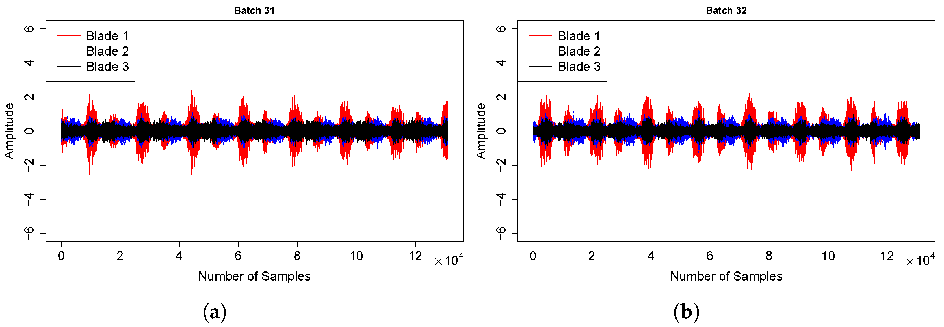
According to feedback from the wind farm, the blade 1 of wind turbine #5 eventually broke. As shown in Table 4, alarms were raised for both monitoring schemes, with the alarm for D m occurring approximately 20 sample points earlier than that for D m S N . We graphed the vibration signals after the first alarm for these two monitoring schemes, as shown in Figure 4 and Figure 5.
As shown in Figure 4 and Figure 5, after the alarm, there is a significant shock in the vibration signal of blade 1, while the amplitude of the vibration signals of blade 2 and blade 3 are close to each other. From the monitoring results for wind turbine #5, D m S N can quickly detect changes in the vibration condition of the blades and provide timely warnings of potential faults, and the detection delay is not significantly longer than that of D m . In terms of the results of wind turbine #1, D m S N shows superior performance in controlling the Type I error. Overall, the proposed self-normalized online monitoring scheme ( D m S N ) performs well compared to D m .

6. Conclusions

Existing nonparametric online monitoring methods suffer from an empirical size distortion when there is a strong temporal dependence between observations. To remedy this issue, we propose a self-normalized online monitoring method based on the empirical characteristic function. We study the asymptotic properties of the monitoring statistic under the null hypothesis as well as the alternative hypothesis, and we employ the multivariate stationary bootstrap method to estimate the critical value of the test. The results of numerical simulations show that the proposed method has significant advantages over existing methods in improving the distortion of the empirical size. It is a more stable test and has good test power. Finally, we demonstrate the practical usefulness of the proposed method through an empirical analysis of the vibration data measured from the blades of two wind turbines.

Supplementary Materials

The following supporting information can be downloaded at https://www.mdpi.com/article/10.3390/math13050710/s1, The supplementary material contains proofs of our main results and additional simulation results. References [5,6,7,11,17,20,27,30,38,39,40,41] are cited in Supplementary Materials.

Author Contributions

Methodology, B.Y.; Software, Y.W.; Formal analysis, Y.W.; Writing—original draft, Y.W.; Writing—review and editing, B.Y.; Supervision, B.Y. All authors have read and agreed to the published version of the manuscript.

Funding

This research is funded by the National Natural Science Foundation of China (11501472).

Data Availability Statement

The data will be made available by the authors on request.

Acknowledgments

We would like to express our gratitude to the three reviewers and the academic editor for their constructive feedback, which greatly contributed to the improvements made in the earlier version of this paper.

Conflicts of Interest

The authors declare no conflicts of interest.

References

  1. Page, E.S. A test for a change in a parameter occurring at an unknown point. Biometrika 1955, 42, 523–527. [Google Scholar] [CrossRef]
  2. Csörgö, M.; Horváth, L. Limit Theorems in Change-Point Analysis; Wiley: Hoboken, NJ, USA, 1997. [Google Scholar]
  3. Aue, A.; Horváth, L. Structural breaks in time series. J. Time Ser. Anal. 2013, 34, 1–16. [Google Scholar] [CrossRef]
  4. Chu, C.S.J.; Stinchcombe, M.; White, H. Monitoring structural change. Econom. J. Econom. Soc. 1996, 64, 1045–1065. [Google Scholar] [CrossRef]
  5. Aue, A.; Kirch, C. The state of cumulative sum sequential changepoint testing 70 years after Page. Biometrika 2024, 111, 367–391. [Google Scholar] [CrossRef]
  6. Horváth, L.; Hušková, M.; Kokoszka, P.; Steinebach, J. Monitoring changes in linear models. J. Stat. Plan. Inference 2004, 126, 225–251. [Google Scholar] [CrossRef]
  7. Aue, A.; Horváth, L.; Kokoszka, P.; Steinebach, J. Monitoring shifts in mean: Asymptotic normality of stopping times. Test 2008, 17, 515–530. [Google Scholar] [CrossRef]
  8. Horváth, L.; Kokoszka, P.; Zhang, A. Monitoring constancy of variance in conditionally heteroskedastic time series. Econom. Theory 2006, 22, 373–402. [Google Scholar] [CrossRef]
  9. Berkes, I.; Gombay, E.; Horváth, L.; Kokoszka, P. Sequential change-point detection in GARCH (p, q) models. Econom. Theory 2004, 20, 1140–1167. [Google Scholar] [CrossRef]
  10. Na, O.; Lee, Y.; Lee, S. Monitoring parameter change in time series models. Stat. Methods Appl. 2011, 20, 171–199. [Google Scholar] [CrossRef]
  11. Kirch, C.; Kamgaing, J.T. On the use of estimating functions in monitoring time series for change points. J. Stat. Plan. Inference 2015, 161, 25–49. [Google Scholar] [CrossRef]
  12. Gösmann, J.; Stoehr, C.; Heiny, J.; Dette, H. Sequential change point detection in high dimensional time series. Electron. J. Stat. 2022, 16, 3608–3671. [Google Scholar] [CrossRef]
  13. Sundararajan, R.R.; Pourahmadi, M. Nonparametric change point detection in multivariate piecewise stationary time series. J. Nonparametr. Stat. 2018, 30, 926–956. [Google Scholar] [CrossRef]
  14. Pein, F.; Sieling, H.; Munk, A. Heterogeneous change point inference. J. R. Stat. Soc. Ser. B Stat. Methodol. 2017, 79, 1207–1227. [Google Scholar] [CrossRef]
  15. Guo, L.; Modarres, R. Two multivariate online change detection models. J. Appl. Stat. 2022, 49, 427–448. [Google Scholar] [CrossRef] [PubMed]
  16. Hušková, M.; Hlávka, Z. Nonparametric sequential monitoring. Seq. Anal. 2012, 31, 278–296. [Google Scholar]
  17. Hlávka, Z.; Hušková, M.; Meintanis, S.G. Change-point methods for multivariate time-series: Paired vectorial observations. Stat. Pap. 2020, 61, 1351–1383. [Google Scholar] [CrossRef]
  18. Kojadinovic, I.; Verdier, G. Nonparametric sequential change-point detection for multivariate time series based on empirical distribution functions. Electron. J. Stat. 2021, 15, 773–829. [Google Scholar] [CrossRef]
  19. Hong, Y.; Wang, X.; Wang, S. Testing strict stationarity with applications to macroeconomic time series. Int. Econ. Rev. 2017, 58, 1227–1277. [Google Scholar] [CrossRef]
  20. Lee, S.; Meintanis, S.G.; Pretorius, C. Monitoring procedures for strict stationarity based on the multivariate characteristic function. J. Multivar. Anal. 2022, 189, 104892. [Google Scholar] [CrossRef]
  21. Horváth, L.; Kokoszka, P.; Wang, S. Monitoring for a change point in a sequence of distributions. Ann. Stat. 2021, 49, 2271–2291. [Google Scholar] [CrossRef]
  22. Holmes, M.; Kojadinovic, I.; Verhoijsen, A. Multi-purpose open-end monitoring procedures for multivariate observations based on the empirical distribution function. J. Time Ser. Anal. 2024, 45, 27–56. [Google Scholar] [CrossRef]
  23. Shao, X.; Zhang, X. Testing for change points in time series. J. Am. Stat. Assoc. 2010, 105, 1228–1240. [Google Scholar] [CrossRef]
  24. Hoga, Y. Monitoring multivariate time series. J. Multivar. Anal. 2017, 155, 105–121. [Google Scholar] [CrossRef]
  25. Dette, H.; Gösmann, J. A likelihood ratio approach to sequential change point detection for a general class of parameters. J. Am. Stat. Assoc. 2020, 115, 1361–1377. [Google Scholar] [CrossRef]
  26. Chan, N.H.; Ng, W.L.; Yau, C.Y. A self-normalized approach to sequential change-point detection for time series. Stat. Sin. 2021, 31, 491–517. [Google Scholar]
  27. Fan, Y.; de Micheaux, P.L.; Penev, S.; Salopek, D. Multivariate nonparametric test of independence. J. Multivar. Anal. 2017, 153, 189–210. [Google Scholar] [CrossRef]
  28. Kirch, C.; Stoehr, C. Sequential change point tests based on U-statistics. Scand. J. Stat. 2022, 49, 1184–1214. [Google Scholar] [CrossRef]
  29. Weber, S.M. Change-Point Procedures for Multivariate Dependent Data. Ph.D. Thesis, Karlsruher Institut für Technologie (KIT), Karlsruhe, Germany, 2017. [Google Scholar]
  30. Kirch, C.; Weber, S. Modified sequential change point procedures based on estimating functions. Electron. J. Stat. 2018, 12, 1579–1613. [Google Scholar] [CrossRef]
  31. Politis, D.N.; Romano, J.P. The stationary bootstrap. J. Am. Stat. Assoc. 1994, 89, 1303–1313. [Google Scholar] [CrossRef]
  32. Politis, D.N.; White, H. Automatic Block-Length Selection for the Dependent Bootstrap. Econom. Rev. 2004, 23, 53–70. [Google Scholar] [CrossRef]
  33. Jentsch, C.; Rao, S.S. A test for second order stationarity of a multivariate time series. J. Econom. 2015, 185, 124–161. [Google Scholar] [CrossRef]
  34. Giacomini, R.; Politis, D.N.; White, H. A warp-speed method for conducting Monte Carlo experiments involving bootstrap estimators. Econom. Theory 2013, 29, 567–589. [Google Scholar] [CrossRef]
  35. Kojadinovic, I. npcp: Some Nonparametric CUSUM Tests for Change-Point Detection in Possibly Multivariate Observations; R Package Version 0.2-6; 2024. Available online: https://CRAN.R-project.org/package=npcp (accessed on 5 December 2024).
  36. James, N.A.; Zhang, W.; Matteson, D.S. ecp: An R Package for Nonparametric Multiple Change Point Analysis of Multivariate Data; R Package Version 3.1.6; 2019. Available online: https://CRAN.R-project.org/package=ecp (accessed on 5 December 2024).
  37. Zhou, Z. Measuring nonlinear dependence in time-series, a distance correlation approach. J. Time Ser. Anal. 2012, 33, 438–457. [Google Scholar] [CrossRef]
  38. Billingsley, P. Convergence of Probability Measures; John Wiley & Sons: Hoboken, NJ, USA, 1968. [Google Scholar]
  39. Hlávka, Z.; Hušková, M.; Kirch, C.; Meintanis, S.G. Fourier–type tests involving martingale difference processes. Econom. Rev. 2017, 36, 468–492. [Google Scholar] [CrossRef]
  40. Ibragimov, I.A.; Hasminskii, R.Z. Statistical Estimation: Asymptotic Theory; Springer Science & Business Media: Berlin/Heidelberg, Germany, 1981. [Google Scholar]
  41. Yokoyama, R. Moment bounds for stationary mixing sequences. Z. Wahrscheinlichkeitstheorie Verwandte Geb. 1980, 52, 45–57. [Google Scholar] [CrossRef]
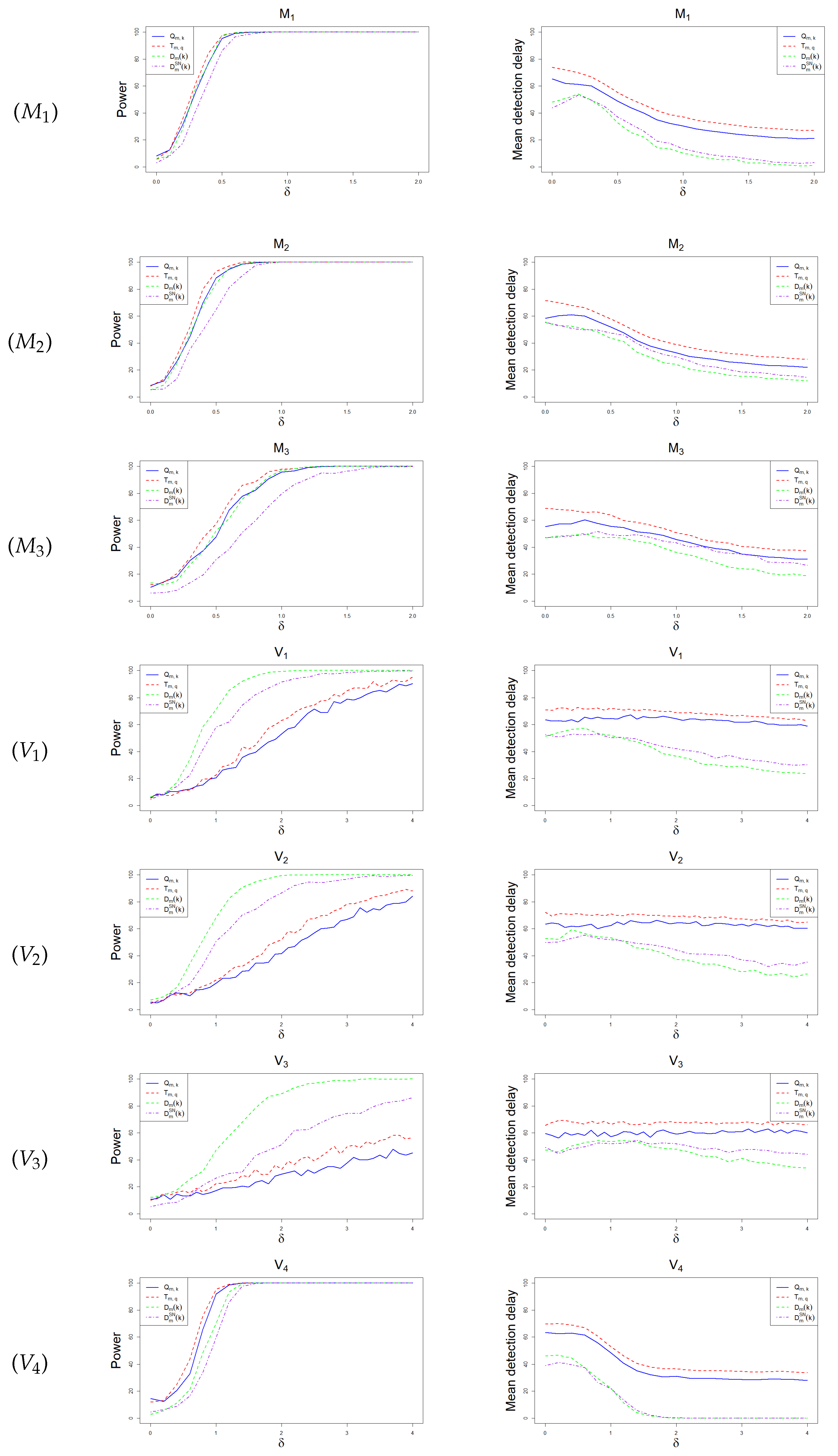
Figure 1. Empirical power and mean detection delay of all monitoring schemes.
Mathematics 13 00710 g001
Figure 2. Vibration signal of the blades of wind turbine #1 during the training phase. (a) The vibration signal from the 1st batch. (b) The vibration signal from the 18th batch.
Mathematics 13 00710 g002
Figure 3. The training sample of wind turbin #1 and its ADCF. The ADCF is implemented using the R package dCovTS (version 1.4). (a) Training sample drawn from the first 18 batches. (b) The ADCF of the training sample.
Mathematics 13 00710 g003
Figure 4. Vibration signal of the blades of wind turbine #5 after the alarm of D m . (a) The vibration signal from the 29th batch. (b) The vibration signal from the 30th batch.
Mathematics 13 00710 g004
Figure 5. Vibration signal of the blades of wind turbine #5 after the alarm of D m S N . (a) The vibration signal from the 31st batch. (b) The vibration signal from the 32nd batch.
Mathematics 13 00710 g005
Table 1. Empirical size of all monitoring schemes (%).
mL N 1 N 2 N 3 N 4 N 5 N 6 N 7 N 8 N 9 N 10 N 11 N 12
Q m , k 10015.77.210.511.522.44.86.77.517.07.29.79.7
25.28.211.614.023.86.05.45.414.26.412.28.6
35.48.79.813.424.45.73.57.716.06.211.810.1
20016.56.68.611.214.96.54.97.012.66.010.69.7
24.76.78.311.417.85.84.95.412.05.89.57.9
35.27.07.910.420.25.85.16.212.25.58.58.5
T m , q 10015.18.010.712.823.64.54.83.510.97.312.39.7
25.87.09.812.824.33.23.93.512.27.09.48.9
35.37.610.513.226.76.24.46.214.76.811.012.2
20014.77.58.011.816.95.24.64.89.55.59.69.1
25.36.48.911.117.34.34.03.710.25.98.67.8
35.07.18.212.018.84.54.65.912.65.39.28.7
D m 10015.87.211.413.931.53.95.99.614.57.013.34.2
25.78.812.216.029.35.16.28.412.66.210.93.4
34.96.39.410.734.03.75.69.714.25.211.53.7
20014.67.39.512.123.33.74.87.29.76.610.44.9
24.07.28.710.119.64.15.59.98.56.811.25.7
35.27.59.210.023.54.44.79.08.57.59.84.8
D m S N 10015.04.05.66.64.03.74.43.63.44.76.34.2
24.55.14.95.75.43.64.14.44.64.66.53.8
35.95.64.34.14.32.93.13.93.74.06.24.5
20014.83.85.03.95.24.13.14.85.84.94.15.2
24.35.34.35.25.42.55.34.53.14.45.25.5
35.14.05.14.63.53.93.94.13.25.85.65.4
Table 2. Empirical power of all monitoring schemes with random change point (%).
mL M 1 , δ = 1 M 2 , δ = 1 M 3 , δ = 1 V 1 , δ = 2 V 2 , δ = 2 V 3 , δ = 2 V 4 , δ = 1
Q m , k 100190.282.563.736.430.520.462.8
291.589.373.140.636.321.665.6
394.691.874.849.242.830.266.3
200194.594.277.953.852.329.679.7
297.496.681.459.357.435.584.2
396.997.186.768.460.041.387.1
T m , q 100199.098.684.345.333.126.582.5
2100.099.995.464.053.333.091.8
3100.0100.098.282.474.646.197.6
2001100.099.995.575.367.636.495.3
2100.0100.099.493.388.352.599.2
3100.0100.099.997.195.573.999.7
D m 100191.187.770.975.370.363.456.7
291.091.880.480.976.164.243.3
394.693.579.679.678.569.745.4
200195.795.283.089.087.374.863.6
298.997.189.090.789.380.257.6
399.198.589.793.090.680.553.7
D m S N 100184.182.552.162.448.837.245.2
282.683.359.169.965.739.143.7
387.488.066.672.169.843.839.8
200195.190.871.378.876.859.347.0
297.594.775.885.082.061.848.0
396.594.582.986.380.766.844.9
Table 3. Monitoring results for wind turbine #1.
Wind Turbine #1L τ ( m ) p Value
D m 1NA0.098
2NA0.076
35090.037
45190.026
56580.039
D m S N 1NA0.468
2NA0.454
3NA0.377
4NA0.355
5NA0.389
Table 4. Monitoring results for wind turbine #5.
Wind Turbine #5L τ ( m ) p Value
D m 1225<0.001
2229<0.001
3230<0.001
D m S N 12460.006
22490.013
32530.021
Disclaimer/Publisher’s Note: The statements, opinions and data contained in all publications are solely those of the individual author(s) and contributor(s) and not of MDPI and/or the editor(s). MDPI and/or the editor(s) disclaim responsibility for any injury to people or property resulting from any ideas, methods, instructions or products referred to in the content.