Abstract
This study explores the risk nexus between the US dollar (USD) market and China’s major financial assets through a co-higher-order testing framework with market regime switching. Specifically, we utilize robust statistical measures such as co-skewness, co-kurtosis, and co-volatility to investigate the connectedness between the US dollar index and a variety of representative financial products in China, including A-shares, the RMB (Chinese Yuan) exchange rate, government bonds with various maturities, and money markets, during the period from 1 January 2010 to 30 June 2023. The empirical results provide evidence of the existence of financial contagion during market regime shifts and also reveal various patterns of cross-market interconnection paths, particularly concerning the third and fourth moment channels. This suggests that the transmission of asymmetric risk and extreme risk, as described in our model, is indeed in place. Furthermore, we discuss practical implications for investors and market regulators in terms of investment decisions and policy coordination.
MSC:
62-08
JEL Code:
G15; G31; G11; G19
1. Introduction
Since their participation in and integration into financial globalization, emerging markets have gradually gained a higher position in the world economy. Through measures such as attracting foreign investment, expanding exports, and promoting domestic reforms, emerging market countries have achieved rapid economic growth. Simultaneously, their financial markets have also experienced rapid development, providing more investment opportunities for global investors. However, emerging markets also face challenges in the process of integrating into financial globalization. For example, the economic foundations of emerging countries are relatively weak, making them vulnerable to external shocks. Emerging market countries also face instability in capital flows. Large inflows of short-term capital may lead to asset bubbles, while capital outflows can trigger financial crises [1,2].
As the largest emerging market in the world, China has been deeply involved in the process of global economic and financial integration over the past number of decades, establishing increasingly close ties with developed country markets such as the United States. On one hand, this has brought in a large influx of capital, promoting the development of the Chinese economy and the prosperity of its capital market. On the other hand, it has also made China’s financial market increasingly sensitive to changes in external market conditions. The US dollar (USD) price, as the most important determinant in global financial markets, can significantly impact the price movements of Chinese financial assets, such as stocks, exchange rates, and bonds, through various channels [3,4].
In parallel, the unexpected COVID-19 pandemic and the Russia–Ukraine war have caused chaos and had ongoing impacts on the global economy, putting market risk spillover on the research agenda of many scholars [5,6,7]. During this period of turmoil, we observe significant market fluctuations in both the United States and China, along with differentiation in their economic performance and macroeconomic policies. As a result, the interactive impact between the financial markets of the two countries is even more complex and unpredictable. Against this background, an important and highly relevant question emerges: how and to what extent does the fluctuation of the US dollar price affect the behavior of major Chinese financial assets, such as Chinese stocks, exchange rates, bonds, and currency markets? The answer to this question is of great importance to investors and policymakers in terms of investment decisions and policy coordination.
Theoretically, the fluctuations of the US dollar price can influence the performance of financial assets in emerging market countries through various paths, including capital flows, trade and investment, debt burdens, and market expectations. For example, when the US dollar strengthens, the currencies of emerging market countries often depreciate relative to it, which can lead to capital outflows and have negative effects on their stock and bond markets. Additionally, as one of the major reserve currencies globally, the exchange rate fluctuations of the US dollar reflect changes in the global economic environment. During periods of global economic prosperity, investors may seek high-risk, high-yield investment opportunities, which can drive capital flows into emerging market countries and have positive effects on their financial assets. Conversely, during periods of global economic downturn, investors may seek safe assets, which can lead to capital outflows from emerging market countries and have adverse effects on their financial assets. Finally, as the debt of emerging market countries is mostly denominated in US dollars, changes in the US dollar exchange rate can impact their debt burden and thus affect the performance of their financial markets [8,9,10].
The related empirical literature on market relationships has come a long way, with the most common and straightforward development being correlation-based tests for contagion [11,12,13]. In a prominent study, Forbes and Rigobon [14] developed a systematic framework based on linear correlations to examine financial contagion and highlight the impact of heteroscedasticity factors on test results. In a similar vein, Luchtenberg and Vu [15] employed the heteroscedasticity-adjusted correlation test to investigate the subprime crisis and founnd strong evidence supporting contagion. Wang and Xiao [16] examined the return and volatility spillover among the US, Chinese, and East Asian stock markets during periods of high volatility, identifying the pathways and magnitude of risk transmission.
However, many studies point out that financial asset returns have non-Gaussian distributions, as they are highly affected by frequent extreme events and crises. This makes return and volatility an incomplete measure of risk. Systematic risk features, such as skewness and kurtosis risk, have the potential to be transmitted through these higher-order risk channels. This problem is also relevant to the relationship between the US dollar and emerging market financial assets and has been verified by some empirical studies [17,18]. Theoretically, spillovers of skewness indicate the spread of asymmetric risk in price movement direction, whereas spillovers of kurtosis evaluate the transmission of extreme risk across markets.
The present study aims to investigate the contagion effect between the US dollar and Chinese financial products using the testing framework proposed by Fry, Martin and Tang [19], and Fry-McKibbin and Hsiao [20]. Specifically, Fry, Martin and Tang [19] first developed an asset pricing model based on the stochastic discount factor model, which accurately represents risk pricing as two components: risk price and risk quantity. The risk quantity is composed of various higher-order conditional moments of the return distribution, including co-skewness. This model highlights the key role of co-higher moments in understanding market interdependencies. Then, the authors designed a co-skewness dependency test method based on Lagrange multipliers by extending the univariate generalized exponential distribution of Lye and Martin [21] to the bivariate case. It is noteworthy that the calculation formula for co-skewness is quite flexible, so the Lagrange multiplier statistic can lead to two alternative forms depending on the order relationship between the first and second moments of the return rates. Fry-McKibbin et al. [22] further improved this testing method to accommodate co-kurtosis and co-volatility and provide a way for testing their interaction. Thus, the testing framework for assessing market risk contagion based on co-higher moments has been established.
Based on this specification, this study aims to examine the risk spillovers from the US dollar market to China’s major asset classes, tracing the timing pattern and channels of this transmission. For this purpose, we select a variety of important categories of financial assets, including the Shanghai composite index (SHI) and the Shenzhen component index (SZI) in the equity market, the 1-month (short-term), 6-month (medium-term) and 1-year (long-term) Shanghai interbank offered rate (SHIBOR) in the money market, the 1-year (short-term), 5-year (medium-term) and 10-year (long-term) government bonds, and the Renminbi exchange rate index in the currency market. These are the most representative financial products that attract widespread attention from investors in the Chinese financial market. We seek to capture evidence of contagion and identify the channels through which risk is transmitted by testing for significant changes in co-high-order moment estimators during market regime switches.
Our work builds on the previous contributions of Wen and Cheng [23], Druck, Magud, and Mariscal [24], and Naresh et al. [18]. These studies all surveyed the transmission of risk from fluctuations in the US dollar to emerging market financial assets. For example, Wen and Cheng [23] demonstrated that the US dollar can act as a safe haven for emerging market stocks. Druck, Magud and Mariscal [24] found that fluctuations in the US dollar primarily affect the performance of emerging market stocks through their impact on commodity prices. Kunkler [25], using the Frankel–Wei regression framework, examined the correlation between the Chinese yuan and the US dollar after the currency reform. The results showed a significant decrease in their correlation level after the Renminbi exchange rate reform in 2015.
In comparison with existing works, the present study advances the literature in the following ways: First, to the best of our knowledge, this is the first attempt to thoroughly and systematically investigate the influence of fluctuations in the US dollar on various financial asset prices in China. Second, the present work provides a robustness analysis of risk transmission, specifically focusing on the higher-order moment channels using the testing framework proposed by Fry-McKibbin and Hsiao [20]. This framework not only allows for thorough and meticulous identification of the channels of influence of higher moments between different markets, but also provides clear indications of the direction of risk transmission. Lastly, the study extends the observation period up to the middle of 2023, fully capturing the recent COVID-19 pandemic and the Russia–Ukraine war, while acknowledging the impact of the crisis events through the identification of different market evolution phases.
2. Methodology
In this section, we introduce high-order moment risk factors into the capital asset pricing model (CAPM) and construct an extended form of the CAPM that incorporates factors such as skewness and kurtosis. At the same time, we present a testing framework for the co-association of moment risks of different orders between dual assets.
2.1. Capital Asset Pricing Model Specification and Co-Higher-Moment Factors
In the standard portfolio selection theory, investors aim to maximize the expected utility subject to variance constraints within a mean-variance framework to achieve an optimal asset allocation [26,27,28]. To incorporate the asymmetry and tail risk of the financial asset pricing process, the traditional capital asset pricing model (CAPM) can be extended to higher-order forms that include higher moments and co-moments of financial asset returns [20,29]. Assuming that investors allocate investments to two assets, the CAPM that includes correlation coefficients, as well as co-skewness, co-kurtosis, and co-volatility coefficients, can be expressed as follows:
where is the return of asset , with , is the market risk-free rate, is the expected value of , and is the risk price for the related risk factors identified by the second, third, and fourth moments of return distribution, with . The loadings in Equation (1) are defined as follows:
where is the proportion of asset in the portfolio and represents the expected utility of portfolio returns. , and are the volatility, skewness and kurtosis of returns, respectively. From Equations (1) and (2), we can see that the CAPM model, including higher-order moments and co-higher-moments, decomposes the expected excess returns of asset 1 into two parts: the risk price and the risk quantity. The risk price, , is determined by the proportion of asset 1 in the portfolio and various risk aversion measures from the investor’s utility function, i.e., , , .
The risk quantity encompasses second-order moments like variance and co-variance, third-order moments like skewness and co-variances, fourth-order moments like kurtosis and co-kurtosis, and co-volatility. The variance terms are and , the covariance term is , the skewness terms are and , the covariances terms are and , the kurtosis terms are and , the co-kurtosis terms are and , and the co-volatility term is .
In reality, if the total sample size is denoted as and the returns of asset 1 and asset 2 at time are denoted as and , respectively, while the sample mean of asset 1′s returns is denoted as and the sample mean of asset 2′s returns is denoted as , , then the two types of co-skewness in Equation (2) can be computed as follows:
the two types of co-kurtosis in Equation (2) can be computed as follows:
and the co-volatility in Equation (2) can be computed as follows:
where measures the contagion effect from a change in the returns of asset 1 to the volatility of asset 2, measures the contagion effect from the volatility of asset 1 to the return of asset 2, measures the contagion effect from a change in the returns of asset 1 to the skewness of asset 2, measures the contagion effect from the skewness of asset 1 to the return of asset 2, and measures the contagion effect from the volatility of asset 1 to the volatility of asset 2.
Fry-McKibbin and Hsiao [20] plotted the risk-return trade-off plane between expected excess returns, variance, skewness and kurtosis after assigning the parameter value in the calculation example. The results illustrated that investors require higher expected excess returns for the volatility risk and kurtosis risk they undertake, but they may tolerate lower expected excess returns to achieve positive skewness. These findings verify the conclusions, as mentioned in previous studies [22,30], that the expected excess returns of risky assets are not only related to their volatility but also closely related to higher-order moments such as skewness, kurtosis, co-skewness, co-kurtosis and co-volatility.
2.2. Contagion Effect Test Based on Co-Higher-Order Moments
In this section, we propose specific methods for testing the contagion effect based on co-higher-order moment factors. Given two markets, and , with the sample period of their returns divided into two segments according to market conditions, denoted as for the first segment and for the second segment, and represent the data size in each segment, respectively. The total sample size is represented by , where . The correlation coefficient of the returns between the two markets during the period is denoted as , and during the period as . To simplify, we further assume that market is the source of contagion, meaning that the risk is transmitted from market to market . represents the sample mean of market ’s returns during the period, represents the sample mean of market ’s returns during the period, represents the sample mean of market ’s returns during the period, and represents the sample mean of market ’s returns during the period. represents the sample standard deviation of market ’s returns during the period, represents the sample standard deviation of market ’s returns during the period, represents the sample standard deviation of market ’s returns during the period, and represents the sample standard deviation of market ’s returns during the period.
2.2.1. Risk Spillover Test Based on Correlation
As discussed previously, we check for cross-market risk contagion using a correlation testing framework. Specifically, we characterize the significant increase in correlation between indicators across different market stages as evidence of financial contagion. However, the presence of a “significant increase in correlation” requires a reliable statistical testing process. Therefore, we employ the statistic proposed by Forbes and Rigobon [14] to test risk transmission from market to market as follows:
where is the adjusted sample correlation coefficient, while is the correlation coefficient between the returns of the two markets during period . can be expressed as follows:
where is the sample correlation coefficient of the returns from two markets during period , is the sample variance of the asset returns of market during period , and is the sample variance of the asset returns of market during period . Under the null hypothesis of no risk spillover, the test statistic asymptotically follows a distribution with 1 degree of freedom [14].
2.2.2. Risk Spillover Test Based on Co-Skewness
Similar to the return-based spillover test mentioned above, the risk spillover test based on co-skewness examines whether there is a significant change in the co-skewness statistic, indicating a contagion effect, taking place through this channel. We can define two different co-skewness risk spillover test statistics, denoted as and , respectively. is to test for contagion where the shocks transmit from a change in the returns of a source market to the volatility of asset returns of a recipient market , while examines the impact of the squared value of market ’s return on the asset returns of market .
where and are market return
where and represent the returns of markets and , respectively, at time during period , represents the sample standard deviation of market in period , represents the sample standard deviation of market in period , and and represent the returns of markets and , respectively, at time during period . The variables and are the orders of the corresponding market returns. Under the null hypothesis of no risk spillover, the test statistics and asymptotically follow a distribution with 1 degree of freedom [20].
2.2.3. Risk Spillover Test Based on Co-Kurtosis
Similarly, the contagion test statistics regarding co-kurtosis can be denoted as and , respectively. measures the impact of a change in the returns for market on the cubed value of returns for market , while assesses the impact of the cubed value of returns for market on the asset returns for market .
where
Under the null hypothesis of no risk spillover, the test statistics and asymptotically follow a distribution with 1 degree of freedom.
2.2.4. Risk Spillover Test Based on Co-Volatility
We denote the test statistic to measure the impact of market ’s volatility on market ’s volatility, which is specifically defined as follows:
where
Under the null hypothesis of no risk spillover, the test statistic asymptotically follows a distribution with 1 degree of freedom [20].
3. Data Selection
We consider the volatility of the US dollar price as the source of shock to Chinese assets and examine its risk contagion effect on nine representative products in Chinese financial markets. The financial assets we examine include the Shanghai composite index (SHI) and the Shenzhen component index (SZI) in the equity market, the 1-month (short-term), 6-month (medium-term) and 1-year (long-term) Shanghai nterbank offered rate (SHIBOR) in the money market, the 1-year (short-term), 5-year (medium-term), and 10-year (medium-term) government bonds, and the Renminbi exchange rate index of the currency market. We collect the indices and data from the DataStream and Wind databases, and perform logarithmic transformation as , denote the asset price at time . The sample period spans from 1 January 2010 to 30 June 2023, fully capturing several important market state transitions, and thus provides a critical testbed for revealing the evolution of contagion processes under different market states.
Daily frequency data are used in our study due to their widespread availability. Moreover, they effectively capture short-term price movements and are easily manageable. Furthermore, daily market return data enable modelers to conduct a wide range of statistical tests, allowing them to analyze the data comprehensively. This facilitates drawing conclusions on various aspects of financial markets, including individual stock behavior and multiple market interactions.
As documented by Jiang, Krishnamurthy and Lustig [31], the influence of the US dollar on the price movement of financial assets heavily depends on the operating regime of US dollar prices. Specifically, the contagion mechanism across assets differs significantly in the scenario of the US dollar appreciating or depreciating. Therefore, in order to present a more nuanced and comprehensive understanding of the influence of US dollar price movement on risk contagion under various market conditions, the entire sample of price series is divided into seven subsamples based on changes in the trend of US dollar prices. Specific details are provided in Table 1.

Table 1.
Subsamples and main trends of US dollar prices. The table reports the regime identification results according to the operating trend of US dollar price movement. We completely define seven consecutive and non-overlapping subperiods within the entire sample period spanning from 1 January 2010 to 30 June 2023.
We calculate the summary statistics for the daily return series of the considered financial assets in both the full sample and the seven different subsamples. The results are reported in Table 2 (for brevity, Table 2 only shows the results for the US dollar index). As Table 2 indicates, the US dollar index returns in the full sample have typical characteristics of financial time series: they are biased (with a highly significant skewness coefficient), have a peaked distribution with thick tails (with a highly significant excess kurtosis coefficient), violate normality assumptions (with a highly significant Jarque–Bera statistic), are stationary and hence suitable for further econometric modeling (with a highly significant augmented Dickey–Fuller statistic), and exhibit some degree of autocorrelation (with a highly significant Q(10) statistic). We also observe differences among the seven subsamples in terms of skewness and autocorrelation. Specifically, five of the seven subsamples do not exhibit significant autocorrelation, while the only two subsamples that show some degree of autocorrelation are Subsample 1 and Subsample 7. However, the autocorrelation in these two subsamples is notably weaker compared to the autocorrelation in the full sample sequence.
Table 2.
Descriptive statistics of USD returns in the whole sample and seven subsamples. J-B is the Jarque–Bera statistic for testing if returns follow a normal distribution. ADF is the augmented Dickey–Fuller unit root test statistic, determined with the minimum AIC criteria for optimal lag selection. Q(10) represents the Ljung–Box Q statistic with a lag order of 10. ***, ** and * denote the significance levels at 1%, 5% and 10%, respectively.
4. Empirical Research
In this section, we conduct an empirical analysis to test the risk spillover effects between US dollar price and major Chinese financial assets. Meanwhile, we put forward specific policy recommendations.
4.1. Data Preprocessing
Following the general concept illustrated in the financial literature [14,15], we define financial contagion as the pure spillover of market risk after removing the interdependence caused by fundamental factors. In this regard, we apply the approach proposed by Forbes and Rigobon [14] by fitting the return series rt into a vector autoregressive process and using the residuals as the test object for risk contagion effects. This allows us to isolate the pure contagion effect while preserving the fundamental interaction relationship between markets.
For the subsample returns ( and ) of the consecutive periods (x and y), we fit the sequence to the following model:
where is the lag operator vector and is the residual term, and subsequently, we use the estimated of to calculate various higher-order moments and risk spillover test statistics. L is the lag order, determined to be L = 5 according to the Akaike information criterion.
4.2. Dynamics of Various Moment Risk Linkages
To obtain a thorough comprehension of the dynamic risk transmission patterns from the US dollar market to representative Chinese financial products, we calculate correlation coefficients, as well as co-covariance, co-skewness, co-kurtosis, and co-volatility coefficients (as defined in Section 2), between the US dollar and nine indicators within each subsample. We then present the results in Figure 1.
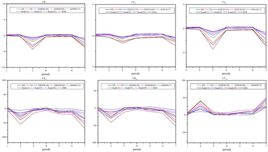
Figure 1.
Time-varying contagion measures with various risk moment factors. We identified seven consecutive and non-overlapping subperiods within the entire sample period spanning from 1 January 2010 to 30 June 2023. The figure illustrates the trends of correlation coefficients and co-higher-moment coefficients between the US dollar and China’s financial products through the first, second, third and fourth moment channels across different subsamples.
From Figure 1, we can observe that the correlation coefficients between the US dollar and other financial assets fluctuate within a narrow range of 0.1–0.5 throughout the entire sample period. However, the time-varying measures of the co-higher-order moment coefficients are much more pronounced. All the higher-order moment test statistics undergo drastic changes around subsample 2 and subsample 6, particularly in the case of the Renminbi exchange rate and the SSI index. These observations suggest that the impact of US dollar shocks on Chinese financial assets is not primarily through the channel of correlation but rather through higher-order moment channels like skewness and kurtosis. Furthermore, the fluctuations in spillover statistics, including correlation coefficients and higher-order moment coefficients, are rather regime-specific.
4.3. Contagion Test Based on Various Co-Higher-Moment Factors
We proceed to examine whether there exists a substantial alteration in the correlation coefficient estimations and several other co-moment statistics of the US dollar and a given financial product when transitioning from subperiod i to subperiod i + 1. As illustrated in Section 2.2, the occurrence of financial contagion is identified as a notable increase in co-moment statistics observed over two consecutive and non-overlapping subsamples.
Table 3 presents the contagion results utilizing the co-higher-order testing framework for the periods identified by regimes of US dollar price movement trends. We observe the highest number of significant contagion statistics for the CK31 estimations, followed by CV22 and FR, with the least significant occurrences seen for CS12 and CS21. This empirical finding supports our hypothesis that the influence of the US dollar on major financial assets in China predominantly operates through channels related to higher-order moments, such as skewness and kurtosis. Regarding specific asset classes, the financial product most broadly and deeply impacted by the US dollar market is the RMB (Chinese Yuan) exchange rate. We notice that with each market regime shift, the relationship between US dollar and RMB exchange rates is significantly reinforced through various channels. For instance, in all six market regime transitions experienced by the US dollar market, both the FR statistic and the CV22 statistic are significant at less than a 5% level, indicating that returns and volatility remain the primary channels through which the RMB exchange rate is influenced by US dollar pricing. The CK31 and CK13 statistics show high significance in period 2—period 3 and period 6—period 7, suggesting that extreme US dollar risk affects the returns of the RMB exchange rate. Meanwhile, extreme returns of the RMB are also highly correlated with the changes in US dollar returns. It is worth noting that period 2—period 3 and period 6—period 7 correspond to the period when the US dollar enters an appreciation phase. This suggests that the impact of the US dollar market on the RMB exchange rate is asymmetric, specifically depending on whether the US dollar price is in an upward or a downward cycle. Overall, the above evidence indicates that, as similar assets, the connection and cross-risk spillover effects between the US dollar and the RMB are considerably strong.
Table 3.
Test results of contagion effect measures. The table presents the results of the contagion test between the US dollar market and Chinese financial products concerning various moment risk factors. The subsample periods are identified by the fluctuation ranges of the US dollar prices, namely appreciation, depreciation, or sideways oscillation. We define a total of seven subperiods, denoted as S1, S2, S3, S4, S5, S6 and S7, respectively. ***, ** and * indicate significance levels at 1%, 5% and 10%, respectively.
The significant impact of the US dollar on China’s equity market mainly occurred in periods 3–4 and 6–7, primarily through the skewness and kurtosis channels. We observe that the CK13 statistics are positive and highly significant for the two equity market indexes during these periods, suggesting that the rise in US dollar returns increases the probability of extreme risk generation in China’s stock market. Additionally, CS21 statistics are also significant in a few cases, indicating that US dollar market volatility is also one of the primary sources of risk in China’s stock market. The above findings have at least two important implications. Firstly, China’s stock market is relatively less connected to international financial markets and is thus not easily affected by international variables such as the US dollar price. Secondly, the appreciation of the US dollar will have a significant adverse effect on China’s stock market, further implying that China’s stock market reacts asymmetrically to external market information; that is, it is more sensitive to negative information.
The impact of the US dollar on the Chinese government bond market is mainly seen in long-term bonds, primarily through first-order and third-order channels. The FR and CK13 show statistical significance at the 5% level during periods 2–3, and CK13 is statistically significant at the 10% level during periods 2–3 and 6–7 for the 10-year government bond yield. As for short- and medium-term bonds, we only observe a few cases of market overshooting at the volatility level. We can conclude from the above results that the majority of bond market investors are fundamentalists who are less influenced by short-term market liquidity and instead focus more on long-term economic prospects.
Regarding the money market, the relationship between the US dollar and the 1-year SHIBOR seems to be relatively constant and unaffected by changes in market conditions. The contagion statistics are generally insignificant, except for CK31 during periods 6–7.
In sum, the above findings reveal the various channels of risk interaction between the US dollar market and Chinese financial products while highlighting the importance of higher-order moment factors in risk spillover. Among the various channels, it is important to note that the contagion between extreme market volatility is the most significant, followed by the connection between volatility and return-related factors. These results largely corroborate the findings of previous studies by Farooque et al. [32], Yarovaya, Brzeszczyński and Lau [33], and Boubaker, Jouini and Lahiani [34]. The negative correlation between the US dollar index and China’s asset prices can be understood through economic theories such as “interest rate parity theory” and “the risk-on, risk-off sentiment”. The former states that when the US dollar strengthens, it typically leads to higher interest rates in the US. This attracts capital flows into US assets, causing a decrease in demand for emerging market assets. As a result, emerging market asset prices tend to fall when the US dollar strengthens. The latter theory suggests that during times of global economic uncertainty or financial market volatility, investors often adopt a “risk-off” sentiment where they seek safe-haven assets like the US dollar. During such periods, the US dollar tends to strengthen, while emerging market assets, which are considered riskier, experience selling pressure and price declines. Furthermore, the higher-order moment linkage pattern between the investigated indicators might reflect the typical reaction of investors to price movements. Specifically, investors in the financial markets often do not have a linear response to market information. Instead, they tend to react collectively when the amount of information accumulates to a certain threshold. This typical reaction can, on the one hand, cause asset prices to exhibit significant bias and jump characteristics. On the other hand, because the change in the US dollar price itself is important information, it can further lead to the appearance of high-order moment dependence characteristics between the US dollar market and emerging markets, such as China.
The above findings have important implications for understanding the economic dynamics of higher-order moment contagion effects, particularly in the context of market stability, investment strategies, and risk management. Traditional financial models, which focus primarily on mean and variance, often overlook the critical role of skewness and kurtosis in capturing asymmetric and extreme risks. However, during periods of market turbulence, such as the COVID-19 pandemic or the Russia–Ukraine war, higher-order moments become indispensable for analyzing risk transmission and its broader economic consequences.
First, higher-order moment contagion can significantly affect market stability. Extreme events in one market, such as sharp fluctuations in the US dollar, can propagate through third and fourth moment channels to other markets, such as China’s stocks, bonds, and currency. For example, US dollar appreciation during a crisis often triggers capital outflows from emerging markets, exacerbating volatility and destabilizing their financial systems. Monitoring co-skewness and co-kurtosis can provide early warning signals of such systemic risks, enabling policymakers to implement preemptive measures.
Second, higher-order moments have important implications for investment strategies. Traditional portfolio diversification strategies, based solely on mean and variance, may fail during crises when assets exhibit strong tail dependencies. Incorporating skewness and kurtosis into portfolio construction can help investors better manage asymmetric and extreme risks. For instance, assets with positive co-skewness may offer downside protection, while those with high co-kurtosis could signal heightened tail risks that require hedging through derivatives or alternative instruments.
Third, risk management practices must evolve to account for higher-order moment contagion. Financial institutions and regulators can use co-volatility and co-kurtosis measures to assess tail risks and ensure adequate capital buffers during stress periods. Macroprudential policies, such as capital adequacy requirements, should also consider higher-order moment risks to enhance financial system resilience.
5. Conclusions
The unprecedented COVID-19 pandemic and the Russia–Ukraine conflict, which evolved into global financial market chaos, have put cross-market risk spillover on the research agenda of many scholars. This issue is particularly prominent for the relationship between advanced financial assets and emerging financial markets due to global risk aversion and increasing asset rebalancing tendencies. In this context, this study checks for the risk contagion between the US dollar market and China’s major financial asset markets through a co-higher-order contagion testing framework with market regime switches. Market dependence patterns are studied from three perspectives: various risk channels, different market regimes, and bidirectional market relations. The empirical results show significant relationships between the US dollar and nine representative financial products of China, while highlighting the risk transmission channels of higher-order moments, including co-skewness, co-kurtosis, and co-volatility. Therefore, among the various risk contagion characteristics between the US dollar and Chinese financial assets, particular attention should be paid to the contagion of extreme risks and directional risks.
The conclusion of this study can provide meaningful reference for market regulators, enabling them to effectively identify financial contagion channels and formulate targeted prevention strategies. It can also provide operational guidance to allow investors to effectively allocate assets and diversify financial market risks. In future research, we plan to construct and evaluate portfolio performance arising from the inclusion of these assets while considering higher-moment linkages.
Author Contributions
Conceptualization, Z.Z.; Methodology, C.Z.; Software, C.Z.; Investigation, J.L.; Resources, J.L. All authors have read and agreed to the published version of the manuscript.
Funding
This research received no external funding.
Data Availability Statement
The data will be made available by the authors on request.
Conflicts of Interest
The authors declare that they have no known competing financial interests or personal relationships that could have appeared to influence the work reported in this paper.
References
- Ahmad, W.; Sehgal, S.; Bhanumurthy, N.R. Eurozone crisis and BRIICKS stock markets: Contagion or market interdependence? Econ. Model 2013, 33, 209–225. [Google Scholar] [CrossRef]
- Bello, J.; Guo, J.; Newaz, M.K. Financial contagion effects of major crises in African stock markets. Int. Rev. Financ. Anal. 2022, 82, 102128. [Google Scholar] [CrossRef]
- Luo, T.; Zhang, L.X.; Sun, H.P.; Bai, J.C. Enhancing exchange rate volatility prediction accuracy: Assessing the influence of different indices on the USD/CNY exchange rate. Financ. Res. Lett. 2023, 58, 104483. [Google Scholar] [CrossRef]
- You, K.F.; Sarantis, N. A twelve-area model for the equilibrium Chinese Yuan/US dollar nominal exchange rate. J. Int. Financ. Mark. Inst. Money 2012, 22, 151–170. [Google Scholar] [CrossRef]
- Chancharat, S.; Sinlapates, P. Dependences and dynamic spillovers across the crude oil and stock markets throughout the COVID-19 pandemic and Russia-Ukraine conflict: Evidence from the ASEAN+6. Financ. Res. Lett. 2023, 57, 104249. [Google Scholar] [CrossRef]
- Wang, Y.; You, X.; Zhang, Y.; Yang, H. Does the risk spillover in global financial markets intensify during major public health emergencies? Evidence from the COVID-19 crisis. Pac.-Basin Financ. J. 2024, 83, 102272. [Google Scholar] [CrossRef]
- Zhang, W.; He, X.; Hamori, S. The impact of the COVID-19 pandemic and Russia-Ukraine war on multiscale spillovers in green finance markets: Evidence from lower and higher order moments. Int. Rev. Financ. Anal. 2023, 89, 102735. [Google Scholar] [CrossRef]
- Ahelegbey, D.F.; Giudici, P.; Hashem, S.Q. Network VAR models to measure financial contagion. N. Am. J. Econ. Financ. 2021, 55, 101318. [Google Scholar] [CrossRef]
- Akhtaruzzaman, M.; Boubaker, S.; Sensoy, A. Financial contagion during COVID-19 crisis. Financ. Res. Lett. 2021, 38, 101604. [Google Scholar] [CrossRef] [PubMed]
- Arfaoui, N.; Yousaf, I. Impact of covid-19 on volatility spillovers across international markets: Evidence from VAR asymmetric Bekk-Garch model. Ann. Financ. Econ. 2022, 17, 2250004. [Google Scholar] [CrossRef]
- Abduraimova, K. Contagion and tail risk in complex financial networks. J. Bank. Financ. 2022, 143, 106560. [Google Scholar] [CrossRef]
- Aboura, S.; Chevallier, J. Tail risk and the return-volatility relation. Res. Int. Bus. Financ. 2018, 46, 16–29. [Google Scholar] [CrossRef]
- Abuzayed, B.; Al-Fayoumi, N. Risk spillover from crude oil prices to GCC stock market returns: New evidence during the COVID-19 outbreak. N. Am. J. Econ. Financ. 2021, 58, 101476. [Google Scholar] [CrossRef]
- Forbes, K.J.; Rigobon, R. No Contagion, Only Interdependence: Measuring Stock Market Comovements. J. Financ. 2002, 57, 2223–2261. [Google Scholar] [CrossRef]
- Luchtenberg, K.F.; Vu, Q.V. The 2008 financial crisis: Stock market contagion and its determinants. Res. Int. Bus. Financ. 2015, 33, 178–203. [Google Scholar] [CrossRef]
- Wang, B.; Xiao, Y. Risk spillovers from China’s and the US stock markets during high-volatility periods: Evidence from East Asianstock markets. Int. Rev. Financ. Anal. 2023, 86, 102538. [Google Scholar] [CrossRef]
- Kilic, E. Contagion effects of U.S. Dollar and Chinese Yuan in forward and spot foreign exchange markets. Econ. Model. 2017, 62, 51–67. [Google Scholar] [CrossRef]
- Naresh, G.; Vasudevan, G.; Mahalakshmi, S.; Thiyagarajan, S. Spillover effect of US dollar on the stock indices of BRICS. Res. Int. Bus. Financ. 2018, 44, 359–368. [Google Scholar] [CrossRef]
- Fry, R.; Martin, V.L.; Tang, C. A new class of tests of contagion with applications. J. Bus. Econ. Stat. 2010, 28, 423–437. [Google Scholar] [CrossRef]
- Fry-Mckibbin, R.; Hsiao, C.Y.L. External Dependence Tests for Contagion; ACT: Bengaluru, India; Centre for Applied Macroeconomic Analysis: Canberra, Australia, 2015. [Google Scholar]
- Lye, J.N.; Martin, V.L. Robust estimation, nonnormalities, and generalized exponential distributions. J. Am. Stat. Assoc. 1993, 88, 261–267. [Google Scholar] [CrossRef]
- Fry-Mckibbin, R.; Martin, V.L.; Tang, C. Financial contagion and asset pricing. J. Bank. Financ. 2014, 47, 296–308. [Google Scholar] [CrossRef]
- Wen, X.Q.; Cheng, H. Which is the safe haven for emerging stock markets, gold or the US dollar? Emerg. Mark. Rev. 2018, 35, 69–90. [Google Scholar] [CrossRef]
- Druck, P.; Magud, N.E.; Mariscal, R. Collateral damage: Dollar strength and emerging markets’ growth. N. Am. J. Econ. Financ. 2018, 43, 97–117. [Google Scholar] [CrossRef]
- Kunkler, M. The Chinese renminbi’s co-movement with the US dollar: Addressing the numéraire issue. Financ. Res. Lett. 2021, 40, 101741. [Google Scholar] [CrossRef]
- Black, F. Capital market equilibrium with restricted borrowing. J. Bus. 1972, 45, 444–455. [Google Scholar] [CrossRef]
- Lintner, J. The valuation of risk assets and the selection of risky investments in stock portfolios and capital budgets. Rev. Econ. Stat. 1965, 47, 13–37. [Google Scholar] [CrossRef]
- Sharpe, W.F. Capital asset prices: A theory of market equilibrium under conditions of risk. J. Financ. 1964, 19, 425–442. [Google Scholar]
- Martellini, L.; Ziemann, V. Improved estimates of higher-order comoments and implications for portfolio selection. Rev. Financ. Stud. 2010, 23, 1467–1502. [Google Scholar] [CrossRef]
- Hwang, S.; Satchel, S.E. Modelling emerging market risk premia using higher moments. Int. J. Financ. Econ. 1999, 4, 271–296. [Google Scholar] [CrossRef]
- Jiang, Z.; Krishnamurthy, A.; Lustig, H. Foreign Safe Asset Demand and the Dollar Exchange Rate. J. Financ. 2021, 76, 1049–1089. [Google Scholar] [CrossRef]
- Farooque, O.A.; Baghdadi, G.; Trinh, H.H.; Khandaker, S. Stock liquidity during COVID-19 crisis: A cross-country analysis of developed and emerging economies, and economic policy uncertainty. Emerg. Mark. Rev. 2023, 55, 101025. [Google Scholar] [CrossRef]
- Yarovaya, L.; Brzeszczyński, J.; Lau CK, M. Intra- and inter-regional return and volatility spillovers across emerging and developed markets: Evidence from stock indices and stock index futures. Int. Rev. Financ. Anal. 2016, 43, 96–114. [Google Scholar] [CrossRef]
- Boubaker, S.; Jouini, J.; Lahiani, A. Financial contagion between the US and selected developed and emerging countries: The case of the subprime crisis. Q. Rev. Econ. Financ. 2016, 61, 14–28. [Google Scholar] [CrossRef]
Disclaimer/Publisher’s Note: The statements, opinions and data contained in all publications are solely those of the individual author(s) and contributor(s) and not of MDPI and/or the editor(s). MDPI and/or the editor(s) disclaim responsibility for any injury to people or property resulting from any ideas, methods, instructions or products referred to in the content. |
© 2025 by the authors. Licensee MDPI, Basel, Switzerland. This article is an open access article distributed under the terms and conditions of the Creative Commons Attribution (CC BY) license (https://creativecommons.org/licenses/by/4.0/).