Article

A Novel High-Efficiency Variable Parameter Double Integration ZNN Model for Time-Varying Sylvester Equations

College of Computer Science and Engineering, Jishou University, Jishou 416000, China
*
Author to whom correspondence should be addressed.
Mathematics 2025, 13(5), 706; https://doi.org/10.3390/math13050706
Submission received: 16 January 2025 / Revised: 15 February 2025 / Accepted: 18 February 2025 / Published: 21 February 2025

Abstract

:
In this paper, a High-Efficiency Variable Parameter Double Integration Zeroing Neural Network (HEVPDIZNN) model combining variable parameter function and double integration is proposed to solve the time-varying Sylvester matrix equations, using the decreasing function with a large initial value as the variable parameter. This design achieves faster convergence and higher accuracy after stabilization.The use of double integral terms ensures that the model has higher solution accuracy and effectively suppresses constant noise, linear noise, and quadratic noise. The article proves the convergence and robustness of the model through theoretical analysis. In the comparison experiments with the existing models (MNTZNN, NTPVZNN, NSVPZNN, NSRNN, and ADIZNN), it is confirmed that HEVPDIZNN has faster convergence speed, the average error at the time of stabilization is about 10 5 times that of the existing models, and it has a better suppression of the linear noise, quadratic noise, and constant noise.

1. Introduction

The Sylvester equation J X + X K = M [1,2,3] has been widely applied in fields such as image processing [4], sound source localization [5,6], and multiple-input multiple-output systems (MIMO) [7]. In recent years, the time-varying Sylvester matrix equation J ( t ) X ( t ) + X ( t ) K ( t ) = M ( t ) has been increasingly applied in dynamic control systems, including robotic control [8,9] and UAV formation [10]. The Bartels–Stewart algorithm [11] and the Hessenberg–Schur method [12] are well-established numerical computational methods that, along with gradient neural networks (GNNs) [3,13], can efficiently solve the static Sylvester matrix equation. When dealing with time-varying matrices in dynamic systems, these methods require continuous coefficient sampling for solving. However, they fail to utilize the trend information of coefficient variations. As a result, they are not suitable for solving the time-varying Sylvester matrix equation.
In 2002, Zhang et al. [14] and others proposed a novel recurrent neural network (OZNN) for efficiently solving time-varying Sylvester matrix equations. By defining the error function as E ( t ) = J ( t ) X ( t ) X ( t ) K ( t ) + M ( t ) , the problem of solving the equation was transformed into designing a method to quickly drive E ( t ) to zero. To achieve this, a derivative function E ˙ ( t ) = λ E ( t ) , λ > 0 was introduced. Initially, the model is randomly assigned an X ( 0 ) , and E ( 0 ) is calculated. Based on E ˙ ( t ) , X ( Δ t ) is iteratively computed ( Δ t is the step size), and the above iterative process is repeated. As t increases to a certain value, E ( t ) approaches zero, and the computed X ( t ) converges to the theoretical solution. This model has been applied in robot trajectory tracking [15], circuit design [16], and angle of arrival (AOA)-based vehicle localization [17]. Although the OZNN model can theoretically converge to a solution quickly, it still has some limitations in practical applications. First, the convergence speed of the OZNN model is limited by the fixed parameter λ , which makes the model less adaptable when dealing with highly dynamic systems. Second, the OZNN model is not robust enough in noisy environments (e.g., constant, linear, and quadratic noise), which leads to a high error level. In addition, the OZNN model fails to fully utilize the trend information of the coefficient changes when dealing with time-varying matrix equations, which limits its application in real dynamic systems.
Dynamic systems require rapid error reduction; therefore, the convergence speed is a critical performance metric for ZNN models when solving time-varying Sylvester matrix equations. Based on the OZNN model, researchers have incorporated activation functions into the error derivative function ( E ˙ ( t ) = λ ψ ( E ( t ) ) , where ψ ( · ) denotes the activation function) to enhance the system’s convergence speed by continuously improving these activation functions. Li and Li [18] proposed the sign-bi-power (SBP) function ψ ( x ) = 1 2 sgn ( x ) ( | x | r + | x | 1 r ) , where sgn ( · ) represents the sign function, to achieve finite-time convergence of the model. Xiao et al. [19] extended SBP by adding a linear term ψ ( x ) = 1 2 | x | m sgn ( x ) + 1 2 x + 1 2 | x | 1 m sgn ( x ) , resulting in a smaller convergence upper bound than that achieved using the SBP activation function. Xiao et al. [20] introduced two new activation functions by adding noise-reducing constant and exponential terms along with increased parameter flexibility, expressed as ψ 1 ( x ) = ( a 1 | x | η + a 2 | x | w ) sgn ( x ) + a 3 x + a 4 sgn ( x ) and ψ 2 ( x ) = b 1 exp ( | x | p ) | x | 1 p sgn ( x ) p + b 2 x + b 3 sgn ( x ) . These activation functions achieved predefined-time convergence and exhibited noise-reduction capabilities. Zhang and Zheng [21] proposed a new activation function by introducing a power parameter k into ψ 1 ( · ) , expressed as ψ ( x ) = ( k 1 | x | η + k 2 | x | ω ) k sgn ( x ) + k 3 x + k 4 sgn ( x ) , which further reduced the convergence upper bound. Han et al. [22] introduced a new parameter p into ψ 2 ( · ) , resulting in a novel nonlinear activation function expressed as ψ ( x ) = a 1 q exp ( q | x | p ) | x | 1 p sgn ( x ) p q + a 2 x + a 3 sgn ( x ) . This activation function achieved fixed-time convergence and exhibited strong robustness under dynamic bounded vanishing and non-vanishing noise. Although the aforementioned activation functions accelerated the model’s convergence, they also led to a certain reduction in solution accuracy due to amplifying error variations.
When fixed λ parameters are used in models similar to the OZNN, they cannot adapt to changes in the error, which limits their flexibility. To address this limitation, researchers have introduced methods combining time-varying parameters with activation functions to solve time-varying Sylvester matrix equations. Zhang et al. [23] introduced an exponential time-varying parameter, which, combined with different activation functions, achieved super-exponential convergence. In Xiao and He [7], a new varying parameter function β exp ( λ 1 a r c c o t ( t ) + λ 2 t ) was proposed, which, when combined with activation functions, endowed the model with predefined convergence characteristics. Gerontitis et al. [24] proposed two new varying parameter functions ( μ 1 ( t ) = γ cosh ( b t ) , μ 2 ( t ) = γ e b t ), enabling the model to achieve finite-time convergence. Jin et al. [25] proposed a new activation function ψ ( x ) = ( k 1 | x | p + k 2 | x | q + k 3 e | x | 1 p ) sgn ( x ) + k 4 x , which, combined with the existing time-varying function β exp ( λ 1 a r c c o t ( t ) + λ 2 t ) , enhanced the model’s fixed-time convergence and robustness. Zheng et al. [8] constructed a faster predefined-time convergence model using a novel activation function ψ ( x ) = ( a 1 F v 1 m ( x ) + a 2 F v 2 m ( x ) ) sgn ( x ) + a 3 x and a new time-varying function ( γ 1 a r c c o t ( t ) + γ 2 t ) τ + τ . Although ZNN models constructed using activation functions and time-varying functions have shown improvements compared to earlier models, their ability to suppress various types of noise, such as large constant noise and bounded noise, is still limited. The convergence time of these models often increases as the noise level rises, and they are ineffective at suppressing linear noise. For monotonically increasing time-varying functions, these models may consume more computational resources and runtime after operating for a certain period.
Unlike the aforementioned methods, Jin et al. [5] solved the time-varying generalized Sylvester matrix equation by combining saturated activation functions with single integration. Lei et al. [26] proposed a new coalescent activation function ψ ( x ) = α sgn θ ( x ) + β x , which, when combined with single integration, achieved fixed-time convergence of the model. While the method combining single integration and activation functions can efficiently suppress constant noise and randomly bounded noise, it fails to eliminate computational errors caused by linear noise. Linear noise is a common phenomenon in various engineering applications, and nonlinear noise can be transformed into linear noise by Taylor’s formula (Liao et al. [27]). To address this issue, Han et al. [28] designed a ZNN model (ADIZNN) combining double integration with activation functions to solve time-varying Sylvester matrix equations, improving the convergence speed and robustness of the model compared to the former methods. However, single or double integration methods, when not combined with activation functions, tend to have relatively slow convergence speeds. On the other hand, combining them with activation functions often reduces the solution accuracy of the model.
Since the double integration term can more effectively capture the dynamic behavior of the system, especially when the system’s state changes rapidly, it provides additional error suppression. This enhances the damping characteristics of the system, thereby improving the stability of the numerical solution. Consequently, it can significantly improve both the accuracy and stability of the solution in cases of highly dynamic or rapidly changing systems. However, the convergence of the pure double integral model is relatively slow, and the model takes more time to reach stability.
The zeroing neural network and its improved models can effectively solve the time-varying Sylvester matrix equation, but there is still much room for improvement in terms of convergence time, noise reduction ability, and solution accuracy. In response to the problems of the above model, which suffers from slow solution speed, large error, and an inability to converge in complex environments, drawing on the foundation of the ADIZNN model, we propose the HEVPDIZNN model, which employs monotonically decreasing time-varying functions with large initial values as the design parameters. This approach supersedes the role of the original activation function in accelerating convergence. As a result of this innovation, through a large number of experiments, we verify the superiority of the model in all aspects. The main contributions of this paper are as follows:
  • A new variable-parameter double integration model (HEVPDIZNN) is proposed to solve time-varying Sylvester matrix equations. This model introduces a novel, simpler, and more efficient time-varying parameter function. Unlike previously used increasing parameter functions, this paper selects a monotonically decreasing function that gradually converges to a constant, improving the feasibility of the model and achieving efficient resource allocation.
  • We provide theoretical proofs of the convergence and robustness of the HEVPDIZNN model under scenarios of no noise, constant noise, and linear noise.
  • Comprehensive experiments are conducted to compare the proposed HEVPDIZNN model with other methods designed in this paper, as well as with existing ZNN models for solving time-varying Sylvester matrix equations. On one hand, the experiments validate that the method of combining monotonically decreasing time-varying parameters with double integration outperforms methods using monotonically increasing time-varying parameters with double integration, fixed-parameter double integration, and activation functions combined with double integration. Additionally, the experiments demonstrate the enhanced performance of the HEVPDIZNN model as the maximum and minimum design parameters increase. On the other hand, the experiments confirm that the HEVPDIZNN model achieves faster solution speed, lower average error, and smaller error variance compared to existing ZNN models under different initial values and noise conditions, including constant noise, linear noise, and quadratic noise.
The remainder of the paper is structured as follows: In Section 2, we describe the time-varying Sylvester matrix equation to be solved and present the design process of the HEVPDIZNN model. In Section 3, we provide the analysis and proofs of the convergence and robustness of the HEVPDIZNN model. In Section 4, we demonstrate through extensive experiments that the HEVPDIZNN model outperforms methods based on monotonically increasing time-varying functions with double integration, fixed-coefficient double integration models, and highlight the enhanced performance of the HEVPDIZNN model as its parameters increase. We also verify the superior convergence speed and accuracy of the HEVPDIZNN model under different initial values and noise conditions compared to existing ZNN models. In Section 5, we apply the HEVPDIZNN model to target tracking, achieving real-time tracking of the target. Section 6 concludes the paper.

2. Problem Description and Model Introduction

In the following section, we describe the time-varying Sylvester matrix equation addressed in this paper. Thereafter, we present the derivation process of the Double Integral-Zeroing Neural Network (DIZNN) model with fixed coefficients. Finally, we design the proposed HEVPDIZNN model.

2.1. Time-Varying Sylvester Matrix Equation

J ( t ) X ( t ) X ( t ) K ( t ) = M ( t )
In this expression, t represents time, and J ( t ) R n × n , K ( t ) R n × n , and M ( t ) R n × n are continuously differentiable time-varying coefficient matrices. The objective of this paper is to solve for X ( t ) R n × n in real-time accurately.

2.2. The Design Process of the HEVPDIZNN Model

For solving the time-varying Sylvester matrix equation using the ZNN (Zhang Neural Network) model, we define a unified error function as follows:
E ( t ) = J ( t ) X ( t ) X ( t ) K ( t ) + M ( t )
In the original ZNN model (OZNN), the derivative of the error function is defined as
E ˙ ( t ) = κ E ( t )
where κ is a positive constant that influences the convergence rate of the model.
Inspired by the work in Liao et al. [27], we first derive the process for the fixed-coefficient double integration ZNN model (DIZNN): First, we define an error function E 1 ( t ) that satisfies the following conditions:
E 1 ( t ) = E ˙ ( t ) + κ E ( t ) E 1 ( t ) = κ 0 t E 1 ( α ) d α
Combining Equations (2) and (4),
E 1 ( t ) = J ( t ) X ˙ ( t ) + J ˙ ( t ) X ( t ) X ˙ ( t ) K ( t ) X ( t ) K ˙ ( t ) + M ˙ ( t ) + κ ( J ( t ) X ( t ) X ( t ) K ( t ) + M ( t ) ) E 1 ( t ) = κ 0 t E 1 ( α ) d α
We further define an error function E 2 ( t ) as follows:
E 2 ( t ) = E 1 ( t ) + κ 0 t E 1 ( α ) d α E 2 ( t ) = κ 0 t E 2 ( α ) d α
Combining Equations (5) and (6), we obtain the following equations:
E 2 ( t ) = J ( t ) X ˙ ( t ) + J ˙ ( t ) X ( t ) X ˙ ( t ) K ( t ) X ( t ) K ˙ ( t ) + M ˙ ( t ) + κ ( J ( t ) X ( t ) X ( t ) K ( t ) + M ( t ) ) + κ 0 t J ( α ) X ˙ ( α ) + J ˙ ( α ) X ( α ) X ˙ ( α ) K ( α ) X ( α ) K ˙ ( α ) + M ˙ ( α ) + κ ( J ( α ) X ( α ) X ( α ) K ( α ) + M ( α ) ) d α E 2 ( t ) = κ 0 t E 2 ( α ) d α
From the above equation, we derive the fixed-coefficient double integration model (DIZNN):
J ( t ) X ˙ ( t ) X ˙ ( t ) K ( t ) = J ˙ ( t ) X ( t ) + X ( t ) K ˙ ( t ) M ˙ ( t ) 3 κ ( J ( t ) X ( t ) X ( t ) K ( t ) + M ( t ) ) 3 κ 2 0 t ( J ( α ) X ( α ) X ( α ) K ( α ) + M ( α ) ) d α κ 3 0 t 0 α ( J ( β ) X ( β ) X ( β ) K ( β ) + M ( β ) ) d β d α
Based on the original OZNN model, we modify the design parameters to be time-varying:
E ˙ ( t ) = Ω ( t ) E ( t )
Next, we present the rationale for converting the design parameters into time-varying functions and the expression of time-varying functions proposed in this paper: in practical applications, the magnitude of design parameters is constrained by hardware resources. For previous time-varying functions, such as κ e c 1 a r c o t ( t ) + c 2 t Xiao and He [7], the model’s design parameters tend to approach infinity as time progresses, making it infeasible for hardware implementation. The optimal approach is to select larger design parameters when the error is significant and smaller design parameters when the error decreases. Therefore, this paper introduces a novel and efficient time-varying function to replace fixed parameters:
Ω ( t ) = τ / ( t + 1 ) + κ
where ( τ ) and ( κ ) are positive numbers that can be used to adjust the maximum and minimum values of the time-varying function. In the experiments of Section 4.1.3, we compared the parameters and came up with the best performing set of parameters ( τ = 2400 , κ = 90 ).
Similar to the derivation approach of the fixed-coefficient double-integral model mentioned above, we define an error function ( E 1 ( t ) = E ˙ ( t ) + Ω ( t ) ( E ( t ) ) ) that satisfies the following conditions:
E 1 ( t ) = J ( t ) X ˙ ( t ) + J ˙ ( t ) X ( t ) X ˙ ( t ) K ( t ) X ( t ) K ˙ ( t ) + M ˙ ( t ) + Ω ( t ) ( J ( t ) X ( t ) X ( t ) K ( t ) + M ( t ) ) E 1 ( t ) = 0 t Ω ( α ) E 1 ( α ) d α
Then, we further define a new error function E 2 ( t ) = E 1 ( t ) + 0 t Ω ( α ) E 1 ( α ) d α , which satisfies the following conditions:
E 2 ( t ) = J ( t ) X ˙ ( t ) + J ˙ ( t ) X ( t ) X ˙ ( t ) K ( t ) X ( t ) K ˙ ( t ) + M ˙ ( t ) + Ω ( t ) ( J ( t ) X ( t ) X ( t ) K ( t ) + M ( t ) ) + 0 t Ω ( α ) ( J ( α ) X ˙ ( α ) + J ˙ ( α ) X ( α ) X ˙ ( α ) K ( α ) X ( α ) K ˙ ( α ) + M ˙ ( α ) + Ω ( α ) ( J ( α ) X ( α ) X ( α ) K ( α ) + M ( α ) ) ) d α E 2 ( t ) = 0 t Ω ( α ) E 2 ( α ) d α
From the above equations, we can obtain the HEVPDIZNN model:
J ( t ) X ˙ ( t ) X ˙ ( t ) K ( t ) = J ˙ ( t ) X ( t ) + X ( t ) K ˙ ( t ) M ˙ ( t ) 3 Ω ( t ) ( J ( t ) X ( t ) X ( t ) K ( t ) + M ( t ) ) + 0 t ( 2 Ω ˙ ( α ) 3 Ω 2 ( α ) ) ( J ( α ) X ( α ) X ( α ) K ( α ) + M ( α ) ) d α + 0 t Ω ( α ) ( 0 α ( Ω ˙ ( β ) Ω 2 ( β ) ) ( J ( β ) X ( β ) X ( β ) K ( β ) + M ( β ) ) d β ) d α
Due to the limitation of hardware devices, external noise is always present, so we need the model to have strong robustness, and below we give the HEVPDIZNN model in the presence of noise:
J ( t ) X ˙ ( t ) X ˙ ( t ) K ( t ) = J ˙ ( t ) X ( t ) + X ( t ) K ˙ ( t ) M ˙ ( t ) 3 Ω ( t ) ( J ( t ) X ( t ) X ( t ) K ( t ) + M ( t ) ) + 0 t ( 2 Ω ˙ ( α ) 3 Ω 2 ( α ) ) ( J ( α ) X ( α ) X ( α ) K ( α ) + M ( α ) ) d α + 0 t Ω ( α ) ( 0 α ( Ω ˙ ( β ) Ω 2 ( β ) ) ( J ( β ) X ( β ) X ( β ) K ( β ) + M ( β ) ) d β ) d α + θ ( t )
where θ is the additive noise, θ ( t ) R n × n . For ease of understanding, we convert Equation (14) to the following form:
X ˙ ( t ) = ( I J ( t ) ) X ˙ ( t ) J ˙ ( t ) X ( t ) + X ˙ ( t ) K ( t ) + X ( t ) K ˙ ( t ) M ˙ ( t ) 3 Ω ( t ) ( J ( t ) X ( t ) X ( t ) K ( t ) + M ( t ) ) + 0 t ( 2 Ω ˙ ( α ) 3 Ω 2 ( α ) ) ( J ( α ) X ( α ) X ( α ) K ( α ) + M ( α ) ) d α + 0 t Ω ( α ) ( 0 α ( Ω ˙ ( β ) Ω 2 ( β ) ) ( J ( β ) X ( β ) X ( β ) K ( β ) + M ( β ) ) d β ) d α + θ ( t )
In Figure 1, we give the specific structure of the time-varying Sylvester matrix equation for model (15).

3. Theoretical Analyses

In this section, the proof procedure for the convergence and robustness of the HEVPDIZNN model used to solve the TVSME problem is given. In order to facilitate the notation in the following theoretical proofs, it is declared here that
j ( t ) , k ( t ) , m ( t ) , e ( t ) , e 1 ( t ) , e 2 ( t ) , a , b , c
respectively, denote the form of each element of the matrix:
J ( t ) , K ( t ) , M ( t ) , E ( t ) , E 1 ( t ) , E 2 ( t ) , A R n × n , B R n × n , C R n × n ,

3.1. Convergence Analysis

Here, we give Theory 1, which proves that the HEVPDIZNN model is able to converge the error in a noise-free environment.
Theory 1. 
Given the coefficient matrices J(t), k(t), M(t), the model is solved for any value of the initial X(0), and the error value of the HEVPDIZNN model is able to converge to zero under noise-free conditions:
lim t E ( t ) F = 0
Proof of Theory 1. 
It is known from the derivation of the HEVPDIZNN model:
E 2 ( t ) = E ˙ ( t ) + Ω ( t ) E ( t ) + 0 t Ω ( α ) ( E ˙ ( α ) + Ω ( α ) E ( α ) ) d α
In addition, the HEVPDIZNN model (13) can be transformed into the following equation:
E 2 ( t ) = 0 t Ω ( α ) E 2 ( α ) d α
The following equation expresses the above Equation (18) in elemental form and derives it as follows:
e ˙ 2 ( t ) = Ω ( t ) e 2 ( t )
Define the Lyapunov function ϑ ( t ) :
ϑ ( t ) = 1 2 e 2 2 ( t )
Its derivative is
ϑ ˙ ( t ) = Ω ( t ) e 2 2 ( t )
Since Ω ( t ) > 0 , ϑ ˙ ( t ) < 0 , at the same time ϑ ( t ) > 0 , according to Lyapunov’s theory of stabilization, we can conclude the following:
lim t | ϑ ( t ) | = lim t | e 2 ( t ) | = 0
According to the definition of the model error function E 1 ( t ) (11), E 2 ( t ) (12), it can be seen that
e 2 ( t ) = e ˙ ( t ) + Ω ( t ) e ( t ) + 0 t Ω ( α ) ( e ˙ ( α ) + Ω ( α ) e ( α ) ) d α
And due to e 1 ( t ) = e ˙ ( t ) + Ω ( t ) e ( t ) , we further deduce
lim t | e 1 ( t ) + 0 t Ω ( α ) e 1 ( α ) d α | = 0
Simultaneous derivation of both sides of the above Equation (25) yields the following equation:
lim t | e ˙ 1 ( t ) + Ω ( t ) e 1 ( t ) | = 0
For Equation (26), we discuss it in two cases. For the first case, if e ˙ 1 ( t ) and Ω ( t ) e 1 ( t ) are of the same sign, then e ˙ 1 ( t ) = e 1 ( t ) = 0 when t , which leads to the following equation:
lim t | e 1 ( t ) | = 0
For the other case,
e ˙ 1 ( t ) = Ω ( t ) e 1 ( t )
Similarly, we define another Lyapunov function ι ( t ) :
ι ( t ) = 1 2 e 1 2 ( t )
and obtain its derivative:
ι ˙ ( t ) = Ω ( t ) e 1 2 ( t )
The same conclusion (27) can be obtained from Lyapunov’s theorem. For e 1 ( t ) = e ˙ ( t ) + Ω ( t ) e ( t ) , the following equation is obtained:
lim t | e ˙ ( t ) + Ω ( t ) e ( t ) | = 0
Similar to the derivation process of conclusion (27), we can obtain the following conclusion:
lim t | e ( t ) | = 0
And we convert the above conclusion into matrix form, i.e.,
lim t E ( t ) F = 0

3.2. Robustness Analysis

In practice, noise is unavoidable, and we cannot ignore the impact of noise on the performance of the model. Next, we provide the model in constant noise and linear noise, which can result in converged error in the validation process.
Theory 2. 
Given a set of coefficient matrices J ( t ) , K ( t ) , M ( t ) , when the HEVPDIZNN model is in the presence of constant noise (N = B), it is able to converge J ( t ) X ( t ) X ( t ) K ( t ) + M ( t ) F to zero for any initial value of the model. The specific expression is
lim t E ( t ) F = 0
Proof of Theory 2. 
The HEVPDIZNN model (14) can be transformed into the following elemental form with constant noise:
e 2 ( t ) = 0 t Ω ( α ) e 2 ( α ) d α + b
Its derivative expression is
e ˙ 2 ( t ) = Ω ( t ) e 2 ( t )
The same process of proof of Equations (18)–(32) leads to the following conclusion:
lim t E ( t ) F = 0
Theory 3. 
Given a set of coefficient matrices J ( t ) , K ( t ) , M ( t ) ,when the HEVPDIZNN model is in the presence of linear noise (N = At + B), it is able to converge J ( t ) X ( t ) X ( t ) K ( t ) + M ( t ) F to zero for any initial value of the model. The specific expression is
lim t E ( t ) F = 0
Proof of Theory 3. 
As in Theorem 2, to obtain Equation (33), we transform the HEVPDIZNN model into the following equation:
e 2 ( t ) = 0 t Ω ( α ) e 2 ( α ) d α + a t + b
Since Ω ( t ) converges to κ as t , in the following, we replace Ω ( t ) by κ . As t tends to infinity, the following equations follow from Equation (35):
e ˙ 2 ( t ) = κ e 2 ( t ) + a e ¨ 2 ( t ) = κ e 2 ( t )
In the same way as Equations (20)–(23), we can introduce
lim t | e ˙ 2 ( t ) | = 0
It is not hard to obtain the following equation:
lim t | e 2 ( t ) | = | a κ |
Joining Equations (24) and (38), there is the following equation which holds when t tends to infinity:
| e ˙ ( t ) + κ e ( t ) + κ 0 t ( e ˙ ( α ) + κ e ( α ) ) d α | = | a κ |
Let L ( t ) = e ˙ ( t ) + κ e ( t ) , then we have
lim t | L ( t ) + κ 0 t L ( α ) d α | = | a κ |
The simultaneous derivation of both sides of Equation (40) with respect to t yields
lim t | L ˙ ( t ) + κ L ( t ) | = 0
The same process of derivation of Equation (31) to Equation (32) leads to the following equation:
lim t | L ( t ) | = 0
Then, we obtain the following equation:
lim t | e ˙ ( t ) + κ e ( t ) | = 0
The same reasoning leads to the following conclusions:
lim t | e ( t ) | = 0
Eventually, the following conclusion can be drawn:
lim t E ( t ) F = 0

4. Experiments

In order to verify the effectiveness of the HEVPDIZNN model for solving the time-varying Sylvester matrix equations and its superiority over the existing models, this section analyzes a number of sets of experiments through two different examples. In Example A, the first subsection conducts experiments on the selection of variable parametric functions for the ZNN model, the second subsection is a comparison experiment between the HEVPDIZNN model and the ZNN model with an activation function combined with dual integration, and the third subsection is an experiment on the parameter selection for the HEVPDIZNN model. In Example B, a comparison is performed with the existing models (modified noise-tolerant zeroing neural network (MNTZNN) [22], noise-tolerant parameter-variable ZNN (NTPVZNN) [25], noise-suppression variable-parameter zeroing neural network (NSVPZNN) [7], noise-suppressing recurrent neural network (NSRNN) [5], and accelerated double-integral zeroing neural network (ADIZNN) [28]) in no noise, constant noise, linear noise, quadratic noise, and other environments for convergence time, solution error, and stability comparison experiments, in which the HEVPDIZNN model selects a set of parameters with moderate performance in Experiment A, and the other models select a set of parameters with optimal performance in the original experiments. In Example C, the models are rigorously compared under noiseless conditions to solve Sylvester matrix equations featuring diverse coefficient matrices. This comparison highlights the robust generalization capability of the models, affirming their effectiveness across a spectrum of coefficient configurations.

4.1. Example A

To solve the time-varying Sylvester matrix equation, we use the following coefficient matrices:
J ( t ) = 2 s i n ( 4 t ) 2 c o s ( 4 t ) 2 c o s ( 4 t ) 2 s i n ( 4 t ) , K ( t ) = s i n ( 2 t ) c o s ( 2 t ) c o s ( 2 t ) s i n ( 2 t )
M ( t ) = c o s ( 2 t ) 2 s i n ( 2 t ) s i n ( 2 t ) c o s ( 2 t ) 2
The initial value of the model solution is uniformly set to X ( 0 ) = 0 2 × 2 .

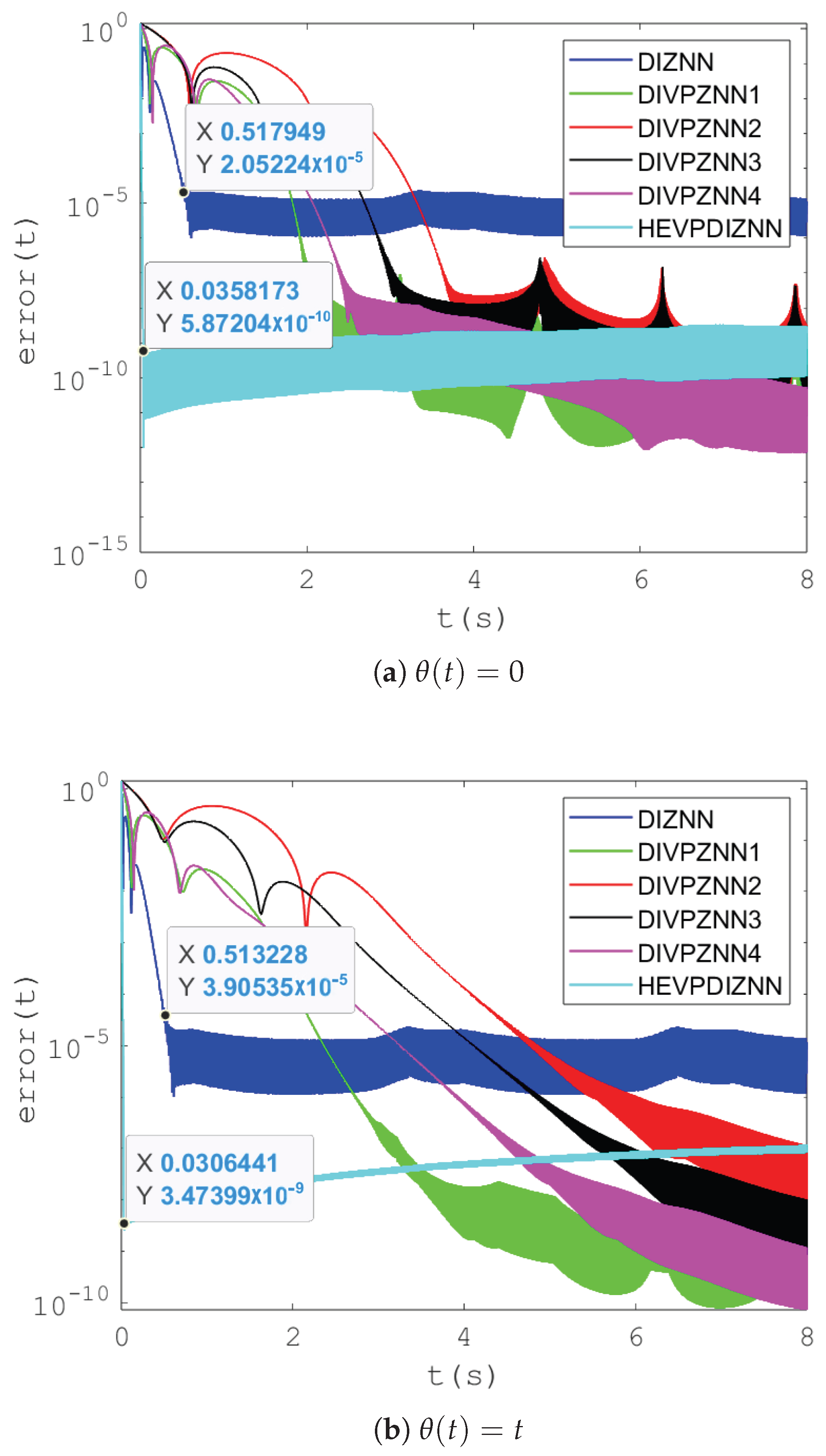
4.1.1. Performance Comparison of DIZNN Models with Various Parameters

In this subsection, we refer to the variable parametric functions proposed in the related literature [7,23,24] and combine them with double integration (DIZNN) to construct ZNN models. We compare these ZNN models based on variable parametric functions with the HEVPDIZNN model. The specific variable parameter functions used are as follows [7,23,24]:
Ω 1 ( t ) = t p + p
Ω 2 ( t ) = γ c o s h ( b t )
Ω 3 ( t ) = γ e b t
Ω 4 ( t ) = β e λ 1 a r c c o t ( t ) + λ 2 t
The experimental parameters follow the original literature and are set as follows: κ = 30 , τ = 800 , p = 5 , γ = β = 1 , b = 1 , λ 1 = 0.8 , λ 2 = 1.2 . In Figure 2, we plot the graphs of various time-varying functions, including those used in the existing literature and the novel time-varying function proposed in this paper. From these graphs, it is evident that only the time-varying function introduced in this paper exhibits a decreasing trend over time. In contrast, the other time-varying functions tend to increase without bounds as time progresses.
Using the time-varying functions (45)–(48) and following the same derivation steps as in Equations (9)–(13), we obtain four time-varying double-integral models, DIVPZNN1, DIVPZNN2, DIVPZNN3, and DIVPZNN4.
Figure 3a carries out the error comparison experiments of the above models in the absence of noise, and the HEVPDIZNN model reaches an order of magnitude of 10 10 in 0.05 s, which is about ten times faster than the second fastest DIZNN model in terms of convergence and about 10 5 times faster than the latter in terms of error. The experimental results show that the HEVPDIZNN model can quickly converge to the steady state, and the error level is significantly lower than that of other existing models. This is mainly attributed to the double integral structure of the model and the design of the decreasing variable parameter function. The double-integral structure enhances the model’s ability to adapt to dynamic changes, while the decreasing variable parameter function provides large parameter values at the initial stage to reduce the error quickly, and then decreases the parameter values as the error decreases to ensure the steady-state accuracy. This design allows the HEVPDIZNN model to achieve a good balance between fast convergence and high accuracy.
In the presence of linear noise (shown in Figure 3b), the HEVPDIZNN model reaches an order of magnitude of 10 9 in about 0.03 s, which is also about ten times faster than the DIZNN model, and the error is about 10 4 times higher than the latter.
Compared with the time-varying double-integral models DIVPZNN1, DIVPZNN2, DIVPZNN3, and DIVPZNN4, these models converge slower, although they are able to reach or even fall below the error level of the HEVPDIZNN model under long runtime. However, in practical experiments, we find that these time-varying double integral models (DIVPZNN1, DIVPZNN2, DIVPZNN3, and DIVPZNN4) suffer from infeasibility, mainly in the form of an excessively long running time.
Table 1 records the comparison of the runtimes of each model under noise-free conditions. Since monotonically increasing variable parametric double integrals require more running time and memory space as the integration interval increases, we choose integration intervals of 8 s, 12 s, and 14 s as examples for our experiments. It is clear that the running time of the monotonically increasing time-varying double-integral model increases exponentially as the integration time increases. For example, the DIVPZNN4 model reaches a running time of 3 h at an integration time of 14 s; even the fastest monotonically increasing time-varying double-integral model, DIVPZNN2, reaches a running time of 829.76 s. In contrast, the DIZNN model and the HEVPDIZNN model not only run fast but also keep the running speed stable. This is due to the fact that the design parameters of DIVPZNNN1 and DIVPZNNN4 increase with time, which makes the computation time and memory consumed increase exponentially, whereas the design parameters of the DIZNN model and the HEVPDIZNN model are constant and decreasing with time until they converge to a constant, respectively, and do not lead to an additional increase in computation time and memory space.
It can be seen that the HEVPDIZNN model has significant advantages in solving the time-varying Sylvester matrix equations in terms of convergence speed, error level, and runtime stability.

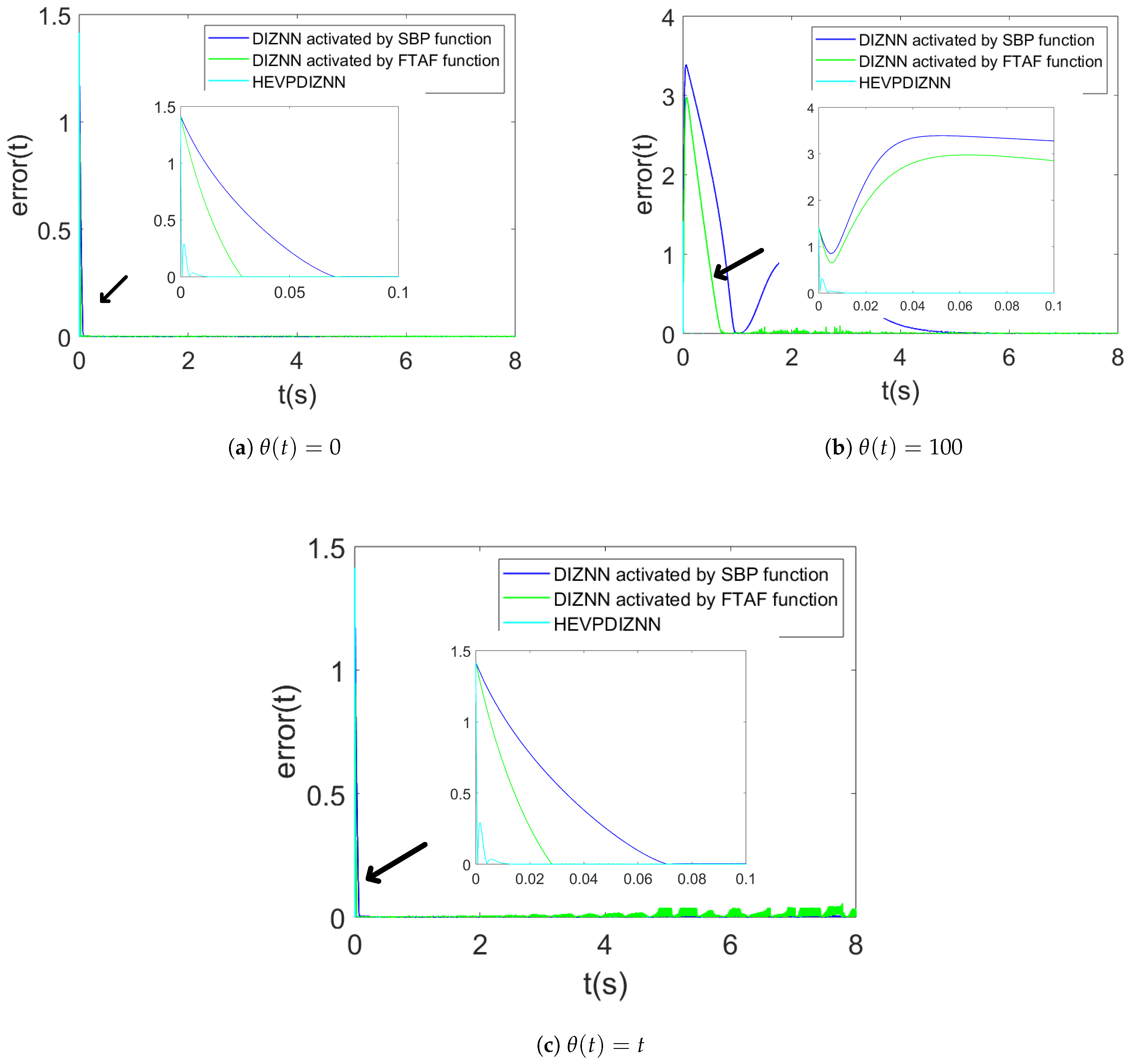
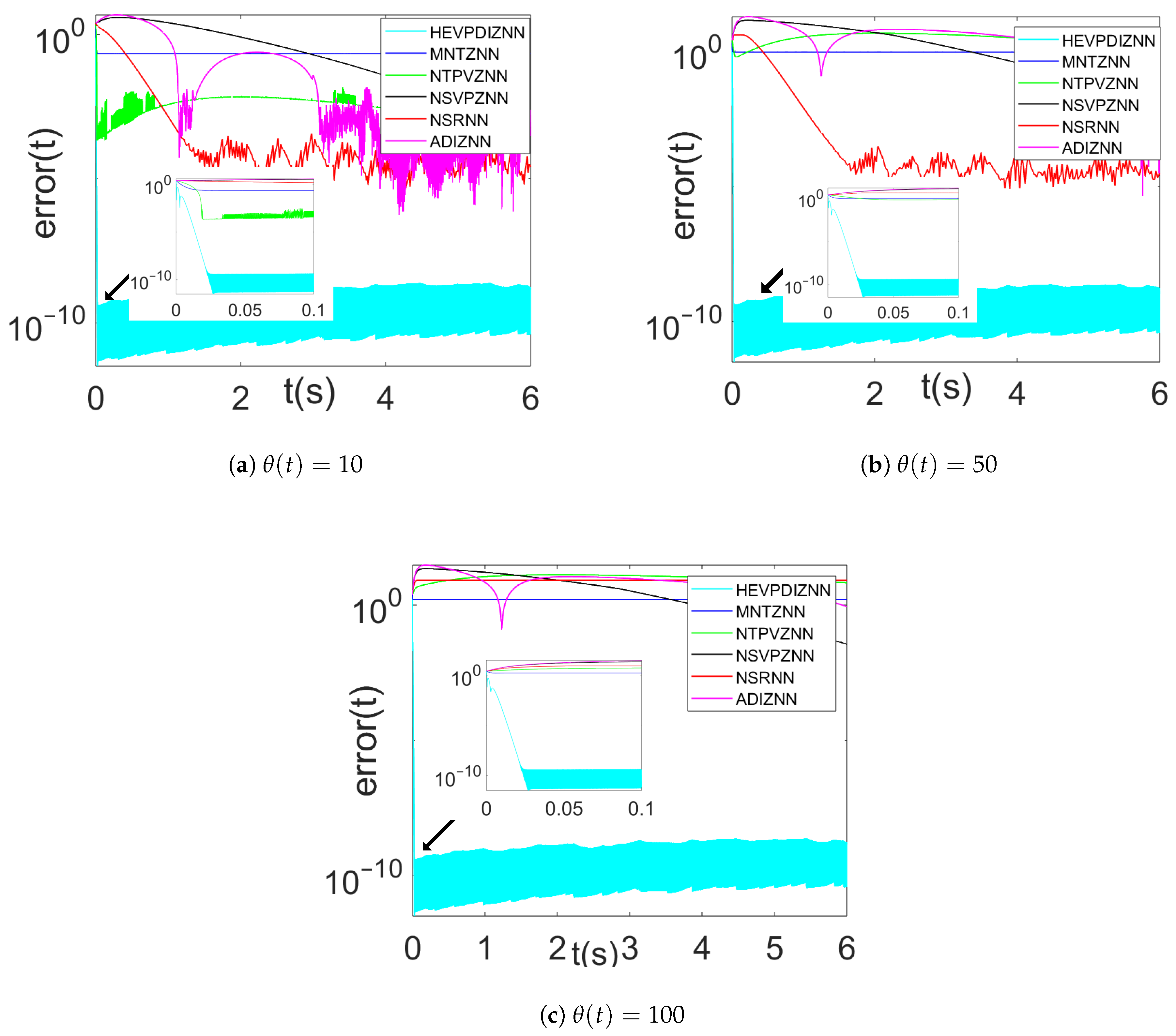
4.1.2. Comparison Between HEVPDIZNN and Activation Function-Based DIZNN Models

Since many ZNN models using activation functions exist, the text considers comparing the ZNN model obtained by combining double integration (DIZNN) and activation functions with the HEVPDIZNN model obtained by combining double integration (DIZNN) and time-varying functions proposed in this paper. Specifically, we choose two activation functions: the SBP ( ψ ( x ) = 1 2 s g n ( x ) ( | x | r + | x | 1 r ), where s g n ( · ) stands for the sign function) [18] and the FTAF (Table 1 ψ 5 ( · ) [28] in Table 1). These activation functions are compared with the performance of the model obtained by combining the DIZNN with the HEVPDIZNN model under noiseless, constant, and linear noise conditions, respectively. The following experimental parameters are set: κ = 30 , τ = 800 , r = q = 2 , p = a 1 = a 2 = a 4 = a 5 = 0.5 .
As shown in Figure 4a–c, the HEVPDIZNN model takes the least amount of time to converge to the same error in each noise and reaches the smallest error in the stabilization stage. Especially in the larger constant noise Figure 4b, the HEVPDIZNN model converges more than 20 times faster than the other models, and the error is about 10 7 than the other models. In Figure 4c, the HEVPDIZNN model decreases the error to about 10 8 at around 0.03 s, while the next DIZNN model with the FTAF activation function decreases the error to about 10 3 at around 0.03 s, and the DIZNN model with SBP activation function drops the error to 10 3 around 0.07 s. Thus, we verify that the model obtained by combining the time-varying function and double integral proposed in this paper converges faster and has higher accuracy than the model obtained by combining the activation function and double integral.

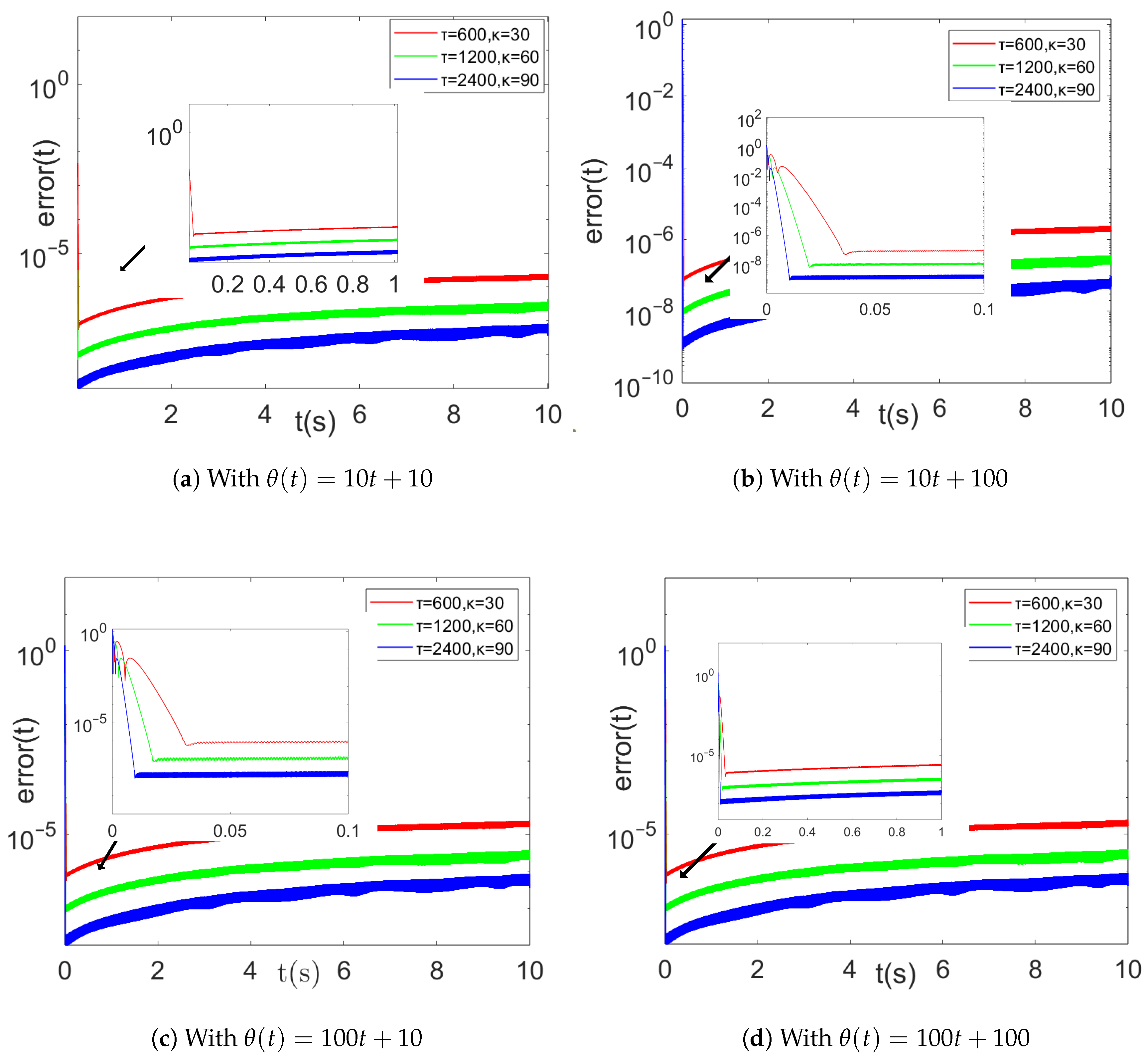
4.1.3. Comparison of Different Parameters of HEVPDIZNN Model

This section aims to explore the effect of the proposed time-varying function combined with double integration for different combinations of maximum and minimum values. In order to visualize the combinations of maximum and minimum values of different variable parameter functions, we give three sets of variable parameter function plots (as shown in Figure 5), and we also design the following sets of different noises to compare the effect of the parameters on the robustness of the model.
  • θ ( t ) = 100
  • θ ( t ) = 10 t + 10
  • θ ( t ) = 10 t + 100
  • θ ( t ) = 100 t + 10
  • θ ( t ) = 100 t + 100
As can be seen from Figure 6, the convergence time and error of the HEVPDIZNN model solved with the same set of parameters do not differ much between the noiseless and constant noise ( θ = 100 ) cases. With increasing parameters, the error decreases from around 10 9 to around 10 10 , while the convergence time increases from 0.01 to 0.045 s.
Figure 7 illustrates the comparison of different variable parameter functions for four different linear noise combinations. For the first two sets of noise (Figure 7a,b), as the model parameters go from small to large, the convergence times of the model are about 0.01, 0.02, and 0.035, respectively. The maximum error can reach below 10 7 , and the minimum error can reach 10 9 . And for the last two sets of noise (Figure 7c,d), the convergence of the model under different parameters time is about the same as the first two sets of experiments, but the error rises, specifically, the maximum error is around 10 6 and the minimum error is 10 8 among the three parameters.
It is clear that as the parameters increase, the model solution error decreases, and the convergence becomes faster.

4.2. Example B

In this set of experiments, we compare the HEVPDIZNN model with the existing ZNN model for solving the time-varying Sylvester matrix equations at different initial values of error, and with different noise. In the following, we expand the coefficient matrix of the Sylvester matrix equation to four dimensions:
J ( t ) = s i n ( t ) s i n ( t ) s i n ( t ) c o s ( t ) s i n ( t ) c o s ( t ) c o s ( t ) s i n ( t ) s i n ( t ) c o s ( t ) c o s ( t ) s i n ( t ) c o s ( t ) s i n ( t ) s i n ( t ) c o s ( t ) , K ( t ) = t 0 0 0 0 1 t + 1 0 0 0 0 t + 2 0 0 0 0 1
M ( t ) = s i n ( 3 t ) s i n ( 3 t ) s i n ( 3 t ) c o s ( 3 t ) 0 s i n ( 3 t ) c o s ( 3 t ) c o s ( 3 t ) 0 0 c o s ( 3 t ) c o s ( 3 t ) 0 0 0 c o s ( 3 t )
Considering the fairness of all the models, all the comparison model parameters adopt the set of better experimental results in the original paper as shown in Table 2. In the table, we give the specific expressions for the activation functions of each model, the form of the design parameters, and the parameter settings used in this experiment.

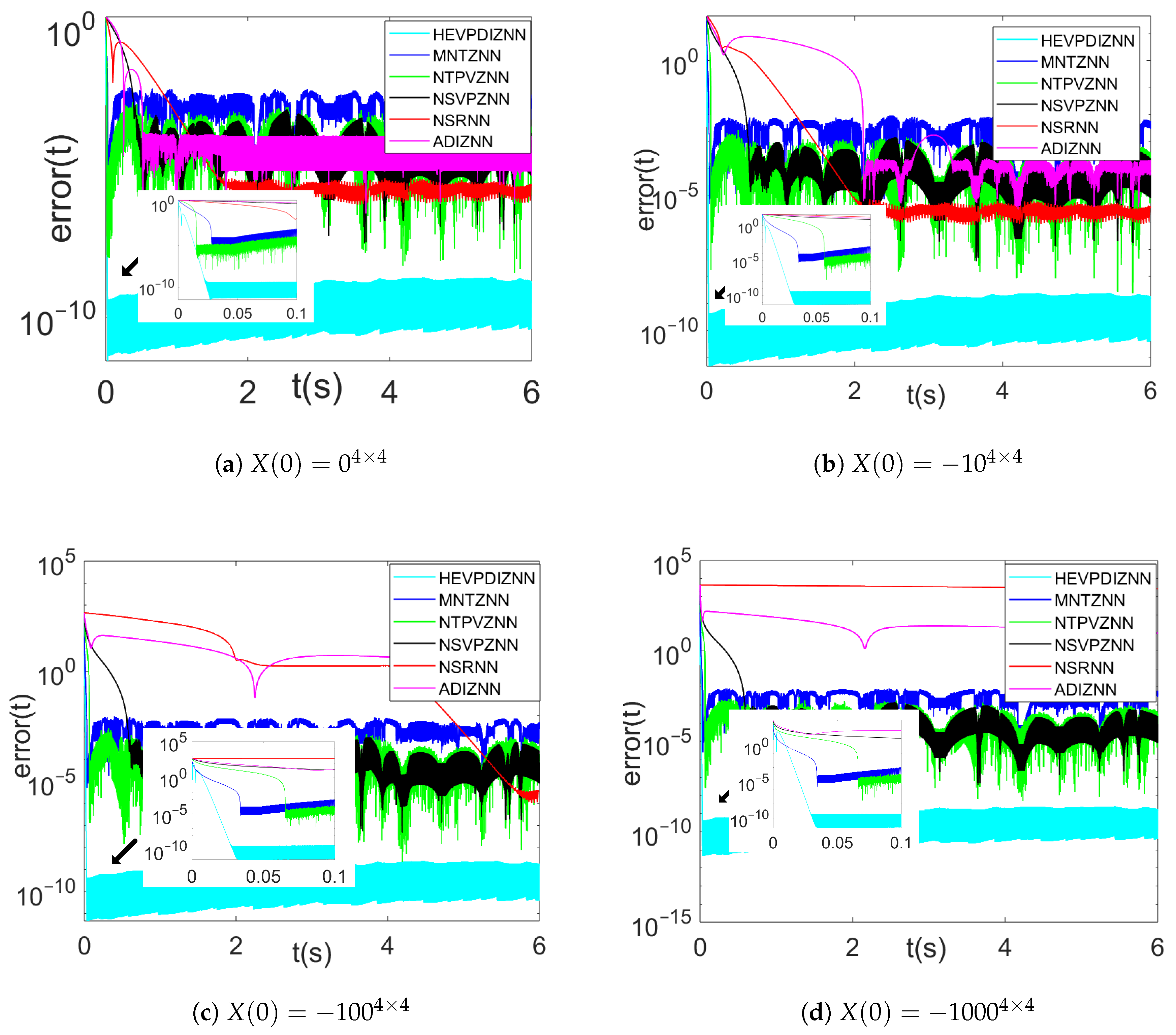
4.2.1. Comparison of Different Error Initial Values in Noiseless

In order to verify that the HEVPDIZNN model is less affected by the error initial value, we compare it with several existing models for solving the time-varying Sylvester matrix equations in the comparison experiments, including the MNTZNN, NTPVZNN, NSVPZNN, NSRNN, and ADIZNN models.
Figure 8a–d show the error convergence of each model for four different initial values of X(0) in the absence of noise. At small initial values of error (as shown in Figure 8a), both the HEVPDIZNN model and the NTPVZNN model reduce the error to about 10 5 within 0.02 s, while the MNTZNN takes about 0.03 s to reduce the error to about 10 4 , which is already a steady state for the NTPVZNN model, and for the MNTZNN model error value in the steady state, the HEVPDIZNN model can stabilize the error value below 10 9 in about 0.025 s. The convergence speeds of the remaining models differ greatly, and the NSRNN model, which has the smallest error value in the steady state, also stops at about 10 6 .
As the initial error value increases, the HEVPDIZNN model still manages to reach the steady state in about 0.025 s. In contrast, the NTPVZNN model performs poorly with large initial errors, as its convergence time in the steady state exceeds 0.06 s and in some cases (Figure 8b–d) lags behind that of the MNTZNN model. The NSRNN and ADIZNN models take a significantly longer time for the model to reach the steady state as the value of the initial error increases, e.g., when X ( 0 ) = 1000 4 × 4 , the convergence time of the above NSRNN and ADIZNN models exceeds the time limit of the experimental run.

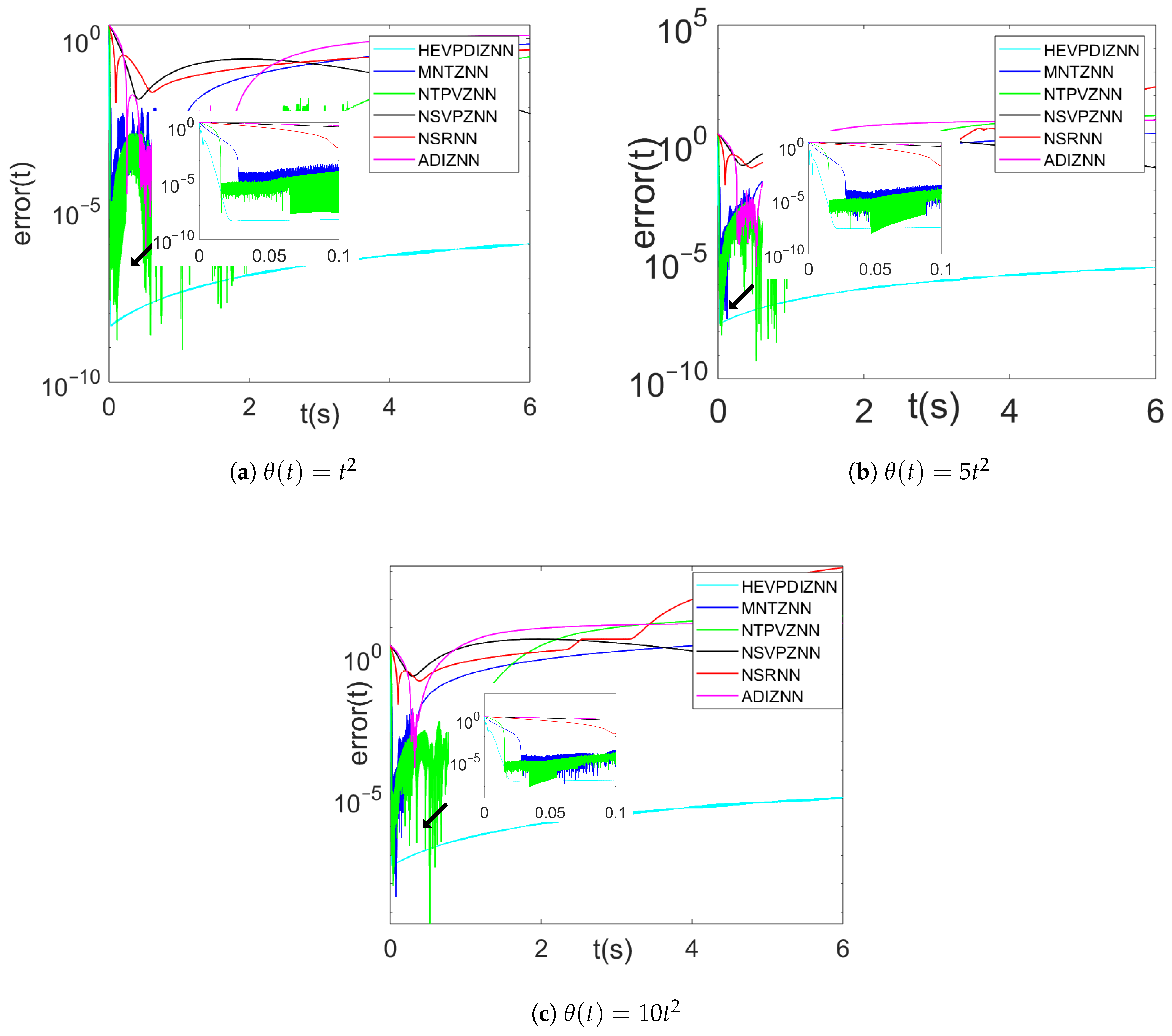
4.2.2. Comparison Under Different Noise Environments
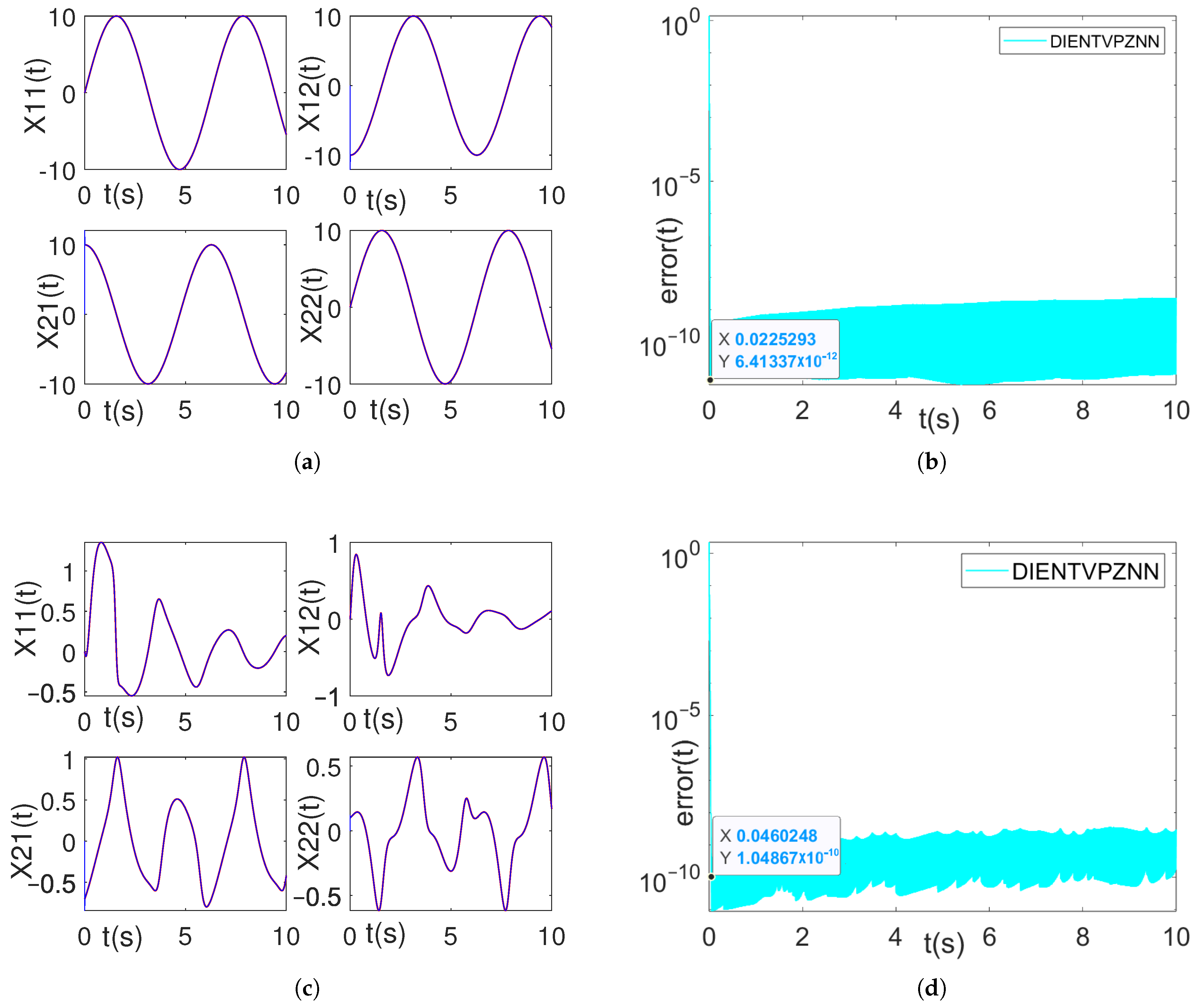
After verifying the robustness of the HEVPDIZNN model to different initial error values, we further explore the performance of the model under different noise conditions.
Figure 9a–c show the error convergence of each model under three constant noise conditions ( θ = 10 , θ = 50 , θ = 100 ), respectively. As can be seen from the figure, the HEVPDIZNN model is almost unaffected by the constant noise, and its time to reach the steady state remains around 0.025 s, and the error value stabilizes below 10 9 . In contrast, the convergence speed and convergence error of the other models are affected to different degrees.
At a constant noise of θ ( t ) = 10 , the average error of the NTPVZNN model rises to around 10 3 at 0.02 s, while the NSRNN and ADIZNN models reach a stable error of around 10 4 at around 1.5 s and 3 s, respectively. At a constant noise of θ ( t ) = 50 , except for the HEVPDIZNN model, only the NSRNN model is able to maintain a certain level of performance, but the convergence time of the rest of the models is out of the experimental range. At a constant noise of θ ( t ) = 100 , even the NSRNN model is unable to reach convergence within 6 s.
Figure 10a–c show the error convergence of each model under three linear noise conditions ( θ = t , θ = 5 t , θ = 10 t ), respectively. As can be seen from the three plots, the convergence rate of the HEVPDIZNN model is almost constant as the linear noise increases, and the error in the steady state stays between 10 6 and 10 8 .
With smaller linear noise θ = t , the MNTZNN model converges the error to about 10 4 within the first second but cannot suppress the noise after 1 second and the error increases and fails to converge. The NTPVZNN model does not show significant linear noise effects for the 6 s that the experiment is carried out.The NSRNN model’s solution error is significantly affected by the linear noise and increases to 10 2 . The convergence rate of the NSVPZNN model decreases significantly and still does not reach a steady state within 6 s. The ADIZNN model, on the other hand, is able to suppress the effect of linear noise in about 0.5 s due to the existence of a double integration structure similar to that of the HEVPDIZNN model.
When the linear noise increases to θ = 5 t , only the ADIZNN model, except for the HEVPDIZNN model, is able to converge to about 10 4 , and the convergence time increases to about 3 s. At a noise of θ = 10 t , the convergence time of the ADIZNN model is further increases to about 4 s, and the rest of the models are unable to converge or fail to converge within the experimental range.
Figure 11a–c show the error convergence of each model in three secondary noise ( θ = t 2 , θ = 5 t 2 , θ = 10 t 2 ) conditions, respectively. As can be seen from the figure, only the HEVPDIZNN model is able to converge within the experimental range in the secondary noise environment. Even when the secondary noise coefficient is 10 ( θ = 10 t 2 ), the error of the HEVPDIZNN model can still be stabilized below 10 5 .
In order to further verify the superiority of the HEVPDIZNN model in solving the time-varying Sylvester matrix equations in terms of the mean and variance of the errors generated by the HEVPDIZNN model, we record the mean and variance of the solution errors when each model in the above experiments reaches a steady state after one second through Table 3 and Table 4. The underlined values in the tables indicate the smallest error mean or variance in that set of data.
Next we will draw the following conclusions from Table 3 and Table 4, in conjunction with the above experiments:
Under no noise, constant noise, linear noise and quadratic noise conditions, the mean and variance of the solution errors of the HEVPDIZNN model are much lower than the rest of the models.
In the noise-free condition, the mean and variance of the error of the HEVPDIZNN model are 7.86 × 10 10 and 5.85 × 10 19 , which are about 10 5 and 10 10 times higher than the best performance of the rest of the comparative models, respectively. For the constant noise θ = 10 , from the data in the table, the error mean and error variance of the HEVPDIZNN model are unaffected by the constant noise, whereas the NSRNN and ADIZNN models are affected to a lesser extent, and the mean values of the remaining models are affected to a greater extent, especially the MNTZNN model which reaches 0.22.
Under linear noise θ = t , the HEVPDIZNN model’s error mean and error variance, although increased, are still much lower than those of the remaining comparison models. Specifically, the error mean of the HEVPDIZNN model is about 10 4 times that of the model with the smallest error mean (ADIZNN) among the remaining comparison models, while the error variance is about 10 10 times that of it. Although the MNTZNN, NTPVZNN, NSVPZNN, and NSRNN models have a suppression effect on the linear noise from the data in the table, the combination of Figure 10b,c shows that the above models fail to converge when the linear noise becomes large.
In the quadratic noise θ = t 2 , the error mean and error variance of the HEVPDIZNN model rise to about 3.32 × 10 7 and 3.26 × 10 7 , respectively, but are still 10 4 times higher than that of the rest of the models with the lowest error mean and the lowest error variance (NTPVZNN) around.

4.3. Example C

This set of experiments will solve the time-varying Sylvester matrix equations under different time-varying coefficient matrices, aiming at verifying that the HEVPDIZNN model has a strong generalization ability and is not only applicable to some specific data. The following are the two new time-varying coefficient matrix datasets added.
The first time-varying coefficient matrix dataset is as follows:
J ( t ) 1 = 0.1 s i n ( t ) 0.1 c o s ( t ) ) 0.1 c o s ( t ) 0.1 s i n ( t ) , K ( t ) 1 = 0.01 s i n ( t ) 0 0 0.02 c o s ( t )
M ( t ) 1 = 0.1 s i n ( t ) s i n ( t ) 1 0.2 c o s ( t ) c o s ( t ) 0.1 s i n ( t ) c o s ( t ) 0.2 s i n ( t ) c o s ( t ) 1
The second time-varying coefficient matrix dataset is as follows:
J ( t ) 2 = sin ( 3 t ) cos ( 3 t ) cos ( 3 t ) sin ( 3 t ) , K ( t ) 2 t 0 0 3
M ( t ) 2 = 2 sin ( 2 t ) 2 cos ( 2 t ) sin ( 2 t ) cos ( 2 t )
The experiments in this section focus on investigating the effect of solving different coefficient matrices on the performance of the HEVPDIZNN model, so we choose to conduct the comparison experiments in a noise-free environment. The experimental parameter settings are ( X ( 0 ) = 0 4 × 4 , τ = 600 , κ = 60 . )
Observations from Figure 12a–d reveal that the model’s solutions align closely with the theoretical solutions across various matrix coefficients within a remarkably short timeframe. Specifically, Figure 12b,d demonstrate that the model efficiently minimizes the error to approximately 6.4 × 10 12 and 1.0 × 10 10 , respectively, at approximately 0.02 s and 0.046 s. Therefore, for different types of coefficient matrices, the model has strong generalization ability.

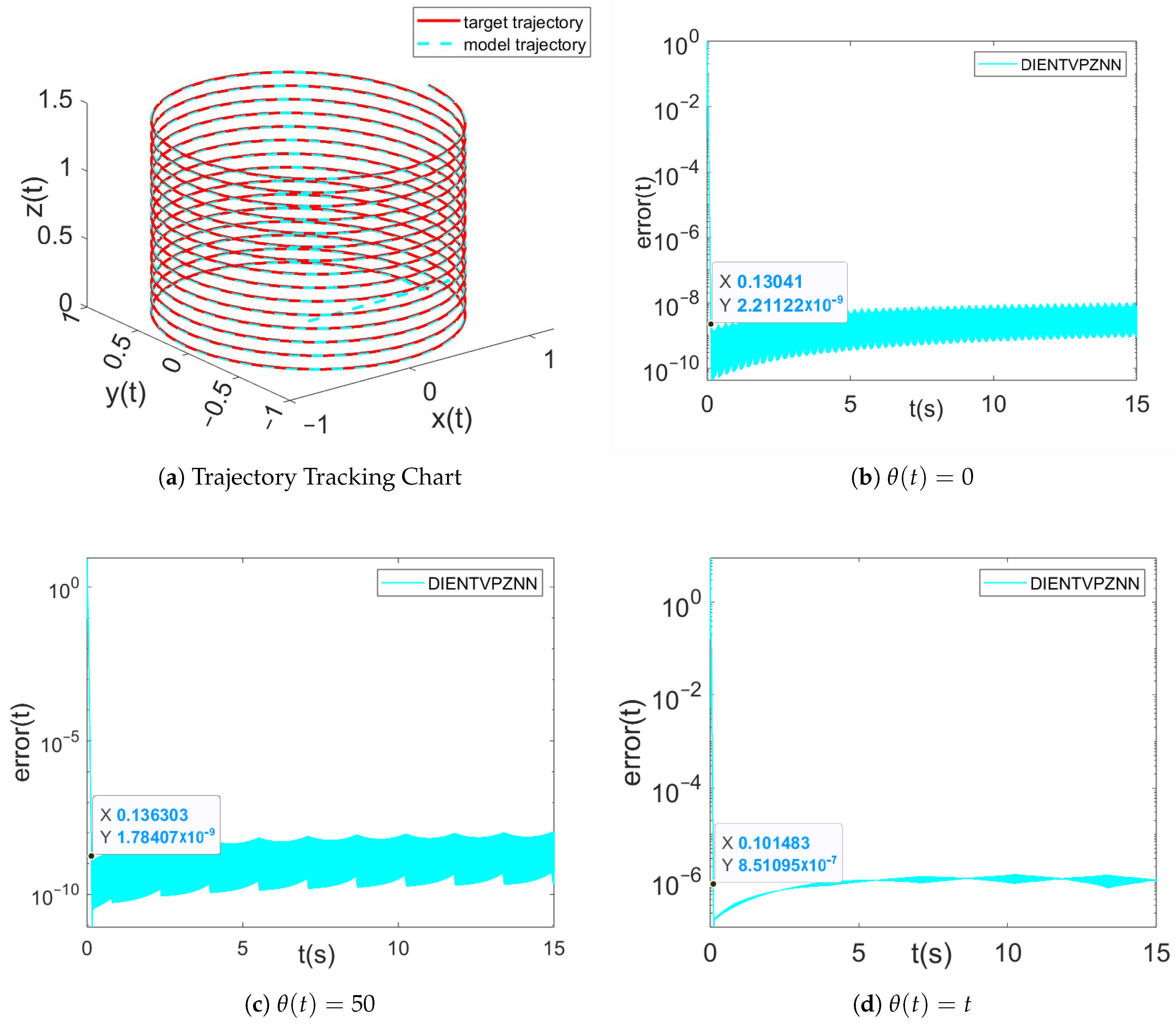
5. Applications in Target Tracking

Target tracking technology, as one of the important technologies in the field of computer vision and machine learning, has a wide range of application scenarios such as real-time monitoring [29], automobile localization [30] and so on. In this paper, the proposed HEVPDIZNN model is applied to target tracking technology, and the following is an example of target tracking application.
Given the following trajectory of the target object on the spatial coordinate axes,
x * ( t ) = c o s ( 2 π t ) y * ( t ) = s i n ( 2 π t ) z * ( t ) = 0.1 t
x(t), y(t), and z(t) are defined as the trajectories solved by the model, where x(0) = 0, y(0) = 0, z(0) = 0. The error function is defined as follows:
E ( t ) = x ( t ) x * ( t ) y ( t ) y * ( t ) z ( t ) z * ( t )
Using the parameters τ = 200 and κ = 20 , we generate the trajectory tracking plot Figure 13a and the error function plot Figure 13b as model solutions in a noise-free environment. It is evident that the model achieves an error reduction to 10 9 within approximately 0.13 s, with the model trajectory closely aligning with the target trajectory. The error function plots Figure 13c,d are derived under constant noise ( θ ( t ) = 50 ) and linear noise ( θ ( t ) = t ), respectively. From Figure 13c,d, it is clear that even under constant noise ( θ ( t ) = 50 ) and linear noise ( θ ( t ) = t ), the model’s solution error remains below approximately 10 8 and 10 6 , respectively, and the convergence time is around 0.1 s. And the convergence times under no noise, constant noise, and linear noise conditions are all around 0.1 s.

6. Conclusions

In this research, we present a new high-efficiency variable parameter double integral zeroed neural network model (HEVPDIZNN) for solving the time-varying Sylvester matrix equation. By combining large initial value time-varying parameter functions with a double integral structure, the model not only achieves fast error convergence and smaller stabilization errors but also demonstrates the effective suppression of linear and quadratic noise.The theoretical analysis proves that the model has good convergence and robustness in various noise environments (no noise, constant noise, and linear noise). The system experimental results further verify the significant advantages of the HEVPDIZNN model in terms of convergence speed, convergence accuracy, and computational efficiency. Through the target tracking case study, we successfully demonstrate the feasibility of the model in practical applications. Moreover, by defining distinct error function equations, the design philosophy akin to that of the HEVPDIZNN model can be extended to address a broader range of time-varying matrix equations. Nevertheless, the study still has some limitations, such as the generalizability of the model, robustness in complex noise environments, and hardware resource limitations. Future research will aim to address these limitations and further optimize the model to improve its performance in a wider range of application scenarios.

Author Contributions

Conceptualization, Y.H. and Z.P.; methodology, Z.P. and Y.H.; software, Z.P., Y.H. and Z.P.; validation, Z.P. and Y.H.; formal analysis, Y.H.; investigation, Z.P.; resources, Y.H.; data curation, Z.P.; writing—original draft preparation, Z.P.; writing—review and editing, Y.H.; visualization, Z.P.; supervision, H.X.; project administration, H.X.; funding acquisition, Y.H. All authors have read and agreed to the published version of the manuscript.

Funding

This work was funded by the National Natural Science Foundation of China under Grant Nos. 62062036, 62066015, and 62466019.

Data Availability Statement

The original contributions presented in the study are included in the article; further inquiries can be directed to the corresponding author..

Conflicts of Interest

The authors declare no conflicts of interest.

References

  1. Hu, D.Y.; Reichel, L. Krylov-subspace methods for the Sylvester equation. Linear Algebra Its Appl. 1992, 172, 283–313. [Google Scholar] [CrossRef]
  2. Darouach, M. Solution to Sylvester equation associated to linear descriptor systems. Syst. Control Lett. 2006, 55, 835–838. [Google Scholar] [CrossRef]
  3. Tan, Z. Fixed-time convergent gradient neural network for solving online Sylvester equation. Mathematics 2022, 10, 3090. [Google Scholar] [CrossRef]
  4. Fang, L.; He, N.; Li, S.; Ghamisi, P.; Benediktsson, J.A. Extinction Profiles Fusion for Hyperspectral Images Classification. IEEE Trans. Geosci. Remote Sens. 2018, 56, 1803–1815. [Google Scholar] [CrossRef]
  5. Jin, L.; Yan, J.; Du, X.; Xiao, X.; Fu, D. RNN for solving time-variant generalized Sylvester equation with applications to robots and acoustic source localization. IEEE Trans. Ind. Inform. 2020, 16, 6359–6369. [Google Scholar] [CrossRef]
  6. Kovalnogov, V.N.; Fedorov, R.V.; Shepelev, I.I.; Sherkunov, V.V.; Simos, T.E.; Mourtas, S.D.; Katsikis, V.N. A novel quaternion linear matrix equation solver through zeroing neural networks with applications to acoustic source tracking. AIMS Math. 2023, 8, 25966–25989. [Google Scholar] [CrossRef]
  7. Xiao, L.; He, Y. A noise-suppression ZNN model with new variable parameter for dynamic Sylvester equation. IEEE Trans. Ind. Inform. 2021, 17, 7513–7522. [Google Scholar] [CrossRef]
  8. Zheng, B.; Han, Z.; Li, C.; Zhang, Z.; Yu, J.; Liu, P.X. A flexible-predefined-time convergence and noise-suppression ZNN for solving time-variant Sylvester equation and its application to robotic arm. Chaos Solitons Fractals 2024, 178, 114285. [Google Scholar] [CrossRef]
  9. Wu, W.; Zhang, Y. Zeroing neural network with coefficient functions and adjustable parameters for solving time-variant Sylvester equation. IEEE Trans. Neural Netw. Learn. Syst. 2022, 35, 6757–6766. [Google Scholar] [CrossRef]
  10. Lee, D.; Thimmaraya, R.; Nataraj, C. Linear Time-varying Tracking Control With Application to Unmanned Aerial Vehicle. In Proceedings of the 2010 American Control Conference, Baltimore, MD, USA, 30 June–2 July 2010. [Google Scholar]
  11. Bartels, R.H.; Stewart, G.W. Algorithm 432 [C2]: Solution of the matrix equation AX + XB = C [F4]. Commun. ACM 1972, 15, 820–826. [Google Scholar] [CrossRef]
  12. Golub, G.; Nash, S.; Van Loan, C. A Hessenberg-Schur method for the problem AX + XB = C. IEEE Trans. Autom. Control 1979, 24, 909–913. [Google Scholar] [CrossRef]
  13. Li, S.; Ma, C. An improved gradient neural network for solving periodic Sylvester matrix equations. J. Frankl. Inst. 2023, 360, 4056–4070. [Google Scholar] [CrossRef]
  14. Zhang, Y.; Jiang, D.; Wang, J. A recurrent neural network for solving Sylvester equation with time-varying coefficients. IEEE Trans. Neural Netw. 2002, 13, 1053–1063. [Google Scholar] [CrossRef] [PubMed]
  15. Jin, J.; Qiu, L. A robust fast convergence zeroing neural network and its applications to dynamic Sylvester equation solving and robot trajectory tracking. J. Frankl. Inst. 2022, 359, 3183–3209. [Google Scholar] [CrossRef]
  16. Jin, J.; Chen, W.; Zhao, L.; Chen, L.; Tang, Z. A nonlinear zeroing neural network and its applications on time-varying linear matrix equations solving, electronic circuit currents computing and robotic manipulator trajectory tracking. Comput. Appl. Math. 2022, 41, 319. [Google Scholar] [CrossRef]
  17. He, Y.; Xiao, L.; Sun, F.; Wang, Y. A variable-parameter ZNN with predefined-time convergence for dynamic complex-valued Lyapunov equation and its application to AOA positioning. Appl. Soft Comput. 2022, 130, 109703. [Google Scholar] [CrossRef]
  18. Li, S.; Li, Y. Nonlinearly activated neural network for solving time-varying complex Sylvester equation. IEEE Trans. Cybern. 2013, 44, 1397–1407. [Google Scholar] [CrossRef]
  19. Xiao, L.; Yi, Q.; Zuo, Q.; He, Y. Improved finite-time zeroing neural networks for time-varying complex Sylvester equation solving. Math. Comput. Simul. 2020, 178, 246–258. [Google Scholar] [CrossRef]
  20. Xiao, L.; Zhang, Y.; Dai, J.; Li, J.; Li, W. New noise-tolerant ZNN models with predefined-time convergence for time-variant Sylvester equation solving. IEEE Trans. Syst. Man. Cybern. Syst. 2019, 51, 3629–3640. [Google Scholar] [CrossRef]
  21. Zhang, M.; Zheng, B. Accelerating noise-tolerant zeroing neural network with fixed-time convergence to solve the time-varying Sylvester equation. Automatica 2022, 135, 109998. [Google Scholar] [CrossRef]
  22. Han, C.; Zheng, B.; Xu, J. A modified noise-tolerant ZNN model for solving time-varying Sylvester equation with its application to robot manipulator. J. Frankl. Inst. 2023, 360, 8633–8650. [Google Scholar] [CrossRef]
  23. Zhang, Z.; Zheng, L.; Weng, J.; Mao, Y.; Lu, W.; Xiao, L. A new varying-parameter recurrent neural-network for online solution of time-varying Sylvester equation. IEEE Trans. Cybern. 2018, 48, 3135–3148. [Google Scholar] [CrossRef] [PubMed]
  24. Gerontitis, D.; Behera, R.; Tzekis, P.; Stanimirović, P. A family of varying-parameter finite-time zeroing neural networks for solving time-varying Sylvester equation and its application. J. Comput. Appl. Math. 2022, 403, 113826. [Google Scholar] [CrossRef]
  25. Jin, J.; Chen, W.; Qiu, L.; Zhu, J.; Liu, H. A noise tolerant parameter-variable zeroing neural network and its applications. Math. Comput. Simul. 2023, 207, 482–498. [Google Scholar] [CrossRef]
  26. Lei, Y.; Luo, J.; Chen, T.; Ding, L.; Liao, B.; Xia, G.; Dai, Z. Nonlinearly activated IEZNN model for solving time-varying Sylvester equation. IEEE Access 2022, 10, 121520–121530. [Google Scholar] [CrossRef]
  27. Liao, B.; Han, L.; Cao, X.; Li, S.; Li, J. Double integral-enhanced Zeroing neural network with linear noise rejection for time-varying matrix inverse. CAAI Trans. Intell. Technol. 2024, 9, 197–210. [Google Scholar] [CrossRef]
  28. Han, L.; He, Y.; Liao, B.; Hua, C. An accelerated double-integral ZNN with resisting linear noise for dynamic Sylvester equation solving and its application to the control of the SFM chaotic system. Axioms 2023, 12, 287. [Google Scholar] [CrossRef]
  29. Mishra, P.K.; Saroha, G. A study on video surveillance system for object detection and tracking. In Proceedings of the 2016 3rd International Conference on Computing for Sustainable Global Development (INDIACom), New Delhi, India, 16–18 March 2016; pp. 221–226. [Google Scholar]
  30. Dai, J.; Li, Y.; Xiao, L.; Jia, L. Zeroing neural network for time-varying linear equations with application to dynamic positioning. IEEE Trans. Ind. Inform. 2021, 18, 1552–1561. [Google Scholar] [CrossRef]
Figure 1. The model structure of the HEVPDIZNN model for solving the time-varying Sylvester matrix equations is shown, where δ 1 = 3 Ω ( t ) , δ 2 = 2 Ω ˙ ( t ) 3 Ω 2 ( t ) , δ 3 = Ω ( t ) ( Ω ˙ ( t ) Ω 2 ( t ) ) , Ω ( t ) = τ / ( t + 1 ) + κ .
Mathematics 13 00706 g001
Figure 2. Time-varying function images; the parameters used refer to those used in the original paper.
Mathematics 13 00706 g002
Figure 3. Comparison of ZNN models obtained by combining three different design parameters with double integration in noiseless and linear noise.
Mathematics 13 00706 g003
Figure 4. Comparison of the HEVPDIZZNN model with the activation function and the DIZNN model.
Mathematics 13 00706 g004
Figure 5. Images of time-varying functions obtained at different combinations of maximum and minimum values of the time-varying function.
Mathematics 13 00706 g005
Figure 6. Comparison of errors ( | | E ( t ) | | F ) obtained by the HEVPDIZNN model using a combination of maximum and minimum values of different design parameters in the absence of noise and constant noise.
Mathematics 13 00706 g006
Figure 7. Comparison of errors ( | | E ( t ) | | F ) obtained by the HEVPDIZNN model using a combination of maximum and minimum values of different design parameters under different combinations of linear noise.
Mathematics 13 00706 g007
Figure 8. Comparison of models with different initialization values (X(0)) in the absence of noise.
Mathematics 13 00706 g008
Figure 9. Comparison of different models under constant noise.
Mathematics 13 00706 g009
Figure 10. Comparison of different models under linear noise.
Mathematics 13 00706 g010
Figure 11. Comparison of different models under quadratic noise.
Mathematics 13 00706 g011
Figure 12. (a,c) The red solid line represents the theoretical solution, and solid blue line represents the model solution. (b,d) The Frobenius norm of the error matrix in the model solving process. The parameter settings are as follows: τ = 600 , κ = 60 . (a) Trajectory tracking for solutions using the first set of coefficient matrices. (b) Error in the solution using the first set of coefficient matrices. (c) Trajectory tracking for solutions using the second set of coefficient matrices. (d) Error in the solution using the second set of coefficient matrices.
Mathematics 13 00706 g012
Figure 13. (a) The red solid line represents the theoretical solution and the cyan dashed line represents the model solution. (bd) The Frobenius norm of the error matrix of the model solved in noiseless ( θ ( t ) = 0 ), constant ( θ ( t ) = 50 ), and linear noise ( θ ( t ) = t ). The parameter settings are τ = 200 , κ = 20 .
Mathematics 13 00706 g013
Table 1. Comparison of time required to run each model.
Integral Time8 s12 s14 s
Model
DIZNN0.36 s0.58 s0.67 s
DIVPZNN192.10 s781.96 s1250.82 s
DIVPZNN24.55 s112.24 s829.76 s
DIVPZNN34.94 s252.27 s1694.25 s
DIVPZNN44.53 s1804.89 s11,817.15 s
HEVPDIZNN9.54 s10.96 s10.43 s
Table 2. Parameters used for each model in the experiment. The group that used the parameter values set in the original experiment with better results.
ModelActivation FunctionDesign ParameterParameter Settings
MNTZNN [22] Ψ 1 ( x ) = a 1 q exp ( q | x | p ) | x | 1 p sgn ( x ) / ( p q ) + a 2 x + a 3 sgn ( x ) γ γ = 1 , a 1 = 2 , a 2 = a 3 = 1 , p = 1 6 , q = 3
NTPVZNN [25] Ψ 2 ( x ) = ( k 1 | x | p + k 2 | x | q + k 3 e | x | p | x | 1 p ) sgn ( x ) + k 4 x α e β 1 arccot ( t ) + β 2 t β 1 = 1 , p = β 2 = 0.2 , q = 2 , k 1 = 15 , α = 1 , k 2 = k 3 = k 4 = 1
NSVPZNN [7] Ψ 3 ( x ) = k 1 | x | p sign ( x ) + k 5 x , if | x | 1 k 2 | x | q sign ( x ) + k 5 x , if | x | > 1 β e λ 1 arccot ( t ) + λ 2 t β = 1 , p = 0.5 , q = 2 , k 1 = k 2 = 0.5 , k 5 = 2 , λ 1 = 0.8 , λ 2 = 1.2
NSRNN [5] Ψ 4 ( x ) = q 2 , if x < q 1 x , if q 1 x q 1 q 2 , if x > q 1 , Ψ 5 ( x ) = q , if x > q x , if q x q q , if x < q ν , μ ν = μ = 10 , q 1 = 1 , q 2 = 5 , q = 5
ADIZNN [28] ψ 5 ( x ) = ( ε 1 | x | p + ε 2 | x | q ) sgn ( x ) + ε 3 x + ε 4 sgn ( x ) ξ , λ μ = 0.5 , σ = 2 , ε 1 = ε 2 = ε 3 = ε 4 = 0.5 , ξ = 2 , λ = 1
HEVPDIZNN (this work)NO κ , τ τ = 1200 , κ = 60
Table 3. Comparison of model error means in different environments (from one second later).
NoiseHEVPDIZNNMNTZNNNTPVZNNNSVPZNNNSRNNADIZNN
07.86 × 10 10 9.92 × 10 4 6.59 × 10 5 7.71 × 10 5 2.57 × 10 5 1.04 × 10 4
107.86 × 10 10 0.22 2.50 × 10 3 1.35 × 10 2 8.22 × 10 5 4.97 × 10 4
t1.83 × 10 8 0.07 1.74 × 10 4 1.40 × 10 3 0.04 1.18 × 10 4
t 2 3.26 × 10 7 0.32 1.10 × 10 3 0.03 0.26 0.01
Note: The underlined values in the tables indicate the smallest error mean or variance in that set of data.
Table 4. Comparison of model error variance in different environments (from one second later).
NoiseHEVPDIZNNMNTZNNNTPVZNNNSVPZNNNSRNNADIZNN
0 5.85 × 10 19 2.31 × 10 6 8.99 × 10 9 1.16 × 10 8 1.14 × 10 8 3.45 × 10 9
10 5.85 × 10 19 2.03 × 10 9 4.33 × 10 6 9.99 × 10 3 5.15 × 10 9 5.52 × 10 8
t 7.92 × 10 14 6.95 × 10 2 1.74 × 10 4 1.40 × 10 3 4.00 × 10 2 1.18 × 10 4
t 2 3.26 × 10 7 3.17 × 10 1 1.10 × 10 3 2.89 × 10 2 2.64 × 10 1 1.01 × 10 2
Note: The underlined values in the tables indicate the smallest error mean or variance in that set of data.
Disclaimer/Publisher’s Note: The statements, opinions and data contained in all publications are solely those of the individual author(s) and contributor(s) and not of MDPI and/or the editor(s). MDPI and/or the editor(s) disclaim responsibility for any injury to people or property resulting from any ideas, methods, instructions or products referred to in the content.

