Article

Travelling Waves in Neural Fields with Continuous and Discontinuous Neuronal Activation

1
Scientific and Educational Center “Fundamental Mathematical Research”, Derzhavin Tambov State University, Tambov 392000, Russia
2
Department of Mathematics, University of Bergen, 5020 Bergen, Norway
3
Department of Sciences and Technology, Norwegian University of Life Sciences, 1432 Ås, Norway
*
Author to whom correspondence should be addressed.
Mathematics 2025, 13(5), 701; https://doi.org/10.3390/math13050701
Submission received: 28 December 2024 / Revised: 17 February 2025 / Accepted: 20 February 2025 / Published: 21 February 2025
(This article belongs to the Section E4: Mathematical Physics)

Abstract

:
The main object of our study is travelling waves in vast neuronal ensembles modelled using neural field equations. We obtained conditions that guarantee the existence of travelling wave solutions and their continuous dependence under the transition from sigmoidal neuronal activation functions to the Heaviside activation function. We, thus, filled the gap between the continuous and the discontinuous approaches to the formalization of the neuronal activation process in studies of travelling waves. We provided conditions for admissibility to operate with simple closed-form expressions for travelling waves, as well as to significantly simplify their numerical investigation. This opens the possibilities of linking characteristics of cortical travelling waves, e.g., the wave shape and the wave speed, to the physiological parameters of the neural medium, e.g., the lengths and the strengths of neuronal connections and the neuronal activation thresholds, in the framework of the neural field theory.

1. Introduction

Travelling waves of electric potentials is the dominant and most well-identified type of electrical activity in the nervous systems of animals, including higher mammals [1] and humans [2,3]. Alpha- and theta-type wave activity propagate in the human cerebral cortex [4]. Some important mechanisms and functions of cortical travelling waves are well explained [5,6] but are still far from being completely understood [7].
In recent works, computer simulations based on the use of simple trigonometric functions, as well as Maxwell’s and Poisson equations, allowed us to assess some parameters of travelling waves (such as the speeds and the wavelengths) by comparing the simulation results with the cortical activity dynamics registered by EEG and MEG [8,9,10,11]. However, this type of study does not allow us to connect cortical travelling wave characteristics (e.g., the wave speed and the wave profile shape) to the physiologically interpretable parameters of the neural media (e.g., the lengths and the strengths of neuronal connections and the neuronal activation thresholds).
A convenient approach to model electrical dynamics of vast ensembles of strongly interconnected neuronal elements are neural field models suggested in the seminal works of H.R. Wilson, J.D. Cowan, and S. Amari [12,13]. The well-known Amari neural field equation (see [13]) is expressed as follows:
t u ( t , x ) = τ u ( t , x ) + R ω ( x y ) f ( u ( t , y ) ) d y , t 0 , x R , τ > 0 .
Here, the value u ( t , x ) characterises electrical activity at time t and position x of the neural field, τ is the relative time constant of the excitation/inhibition processes, the so-called connectivity function ω describes the coupling strengths in the neural field, and the firing rate function f formalises the transition of neurons between the rest state and the active state. The typically used connectivity functions are even, continuous, and integrable and often taken as linear combinations of exponentially decaying functions. Firing rate functions are taken to be smooth functions of sigmoidal shape. These assumptions, of course, agree with the statistical physics nature of mean field models.
The first study of moving patterns of neuronal activity in the framework of neural field equations was carried out in the work of G.B. Ermentrout and J.B. McLeod [14], where the travelling fronts realizing the transition of the rest state of neuronal populations to the active state were studied. However, travelling front solutions have no physiological relevance due to the absence of the so-called refractory phase in the corresponding neural waves (see Figure 1a). In this respect, a more realistic pattern of moving activity is represented by the so-called travelling waves [15] that are also referred to as travelling pulses (see Figure 1b).
The first study of travelling wave solutions in neural fields was given in [16], where a slow local negative feedback component v modelling effects, e.g., spike frequency adaptation or synaptic depression, was added to the synaptic spatial coupling described by (1):
t u ( t , x ) = τ u ( t , x ) + R ω ( x y ) f β ( u ( t , y ) ) d y v ( t , x ) , 1 ϵ t v ( t , x ) = u ( t , x ) σ v ( t , x ) , t 0 , x R , 0 < ϵ 1 , σ > 0 .
Here, the rate and the decay of the negative feedback v are given by ϵ and σ , respectively. Note that, in all results below, the assumption 0 < ϵ 1 can be specified as 0 < ϵ < ( σ + 4 ) 1 , but, in some cases, this estimate can be more general. In the setting (2), the connectivity function is typically considered non-negative due to the formalization of the inhibitory effects in the neural field by the function v.
The authors of [16] examined the existence of travelling waves in the cases when the firing rate function f was represented by both a sigmoidal firing rate function and the Heaviside function.
It should be noted that the substitution of Heaviside-type firing rate functions was often exploited in the mathematical neuroscience community, allowing us to obtain closed-form expressions for many types of stationary solutions, to find their existence conditions, and to assess their stability (see, e.g., [13,17,18,19]). In the studies of travelling waves, both sigmoid-type and Heaviside-type functions were extensively exploited. Numerical investigation of travelling waves in the case of the Heaviside firing rate function was carried out in [20]. The authors of [21] examined the existence and stability of travelling wave solutions in the Heaviside firing rate case. The stability of travelling waves using the Evans function approach, wave stability and bifurcation as functions of system parameters, including the speed and strength of synaptic coupling and the speed of axonal signals, were studied in [22] in the discontinuous neuronal activation setting. A numerical study on travelling anti-wave (moving region with lowered activity) in the case of the smooth firing rate function was carried out in [23]. The existence and exponential stability of travelling waves were investigated in [24] for the case of a Heaviside-type neuronal activation. In [25], the stability and bifurcations of travelling waves using center manifold reduction were examined for neural field equations with discontinuous firing rate functions. A detailed study of the linear stability of travelling wave solutions using several Evans function constructions and nonlinear stability based on the spectral stability property of travelling waves was carried out in [26] for the Heaviside neuronal activation case. In the same setting, the authors of [27] investigated how wave shape, speed, and stability vary as the synaptic coupling and the model parameters change. One interesting point observed was that the travelling wave stability index function can be defined through the wave speed index function. The existence and stability of travelling waves and wave propagation failure, depending on the strength of a stationary external input, were studied in [28] for the both sigmoidal and Heaviside-type firing rate functions. Travelling wave propagation failure due to the growth of the heterogeneity of the periodically modulated connectivity function was investigated in [29] in both the continuous and discontinuous formalizations of neuronal activation.
However, no connection between the results obtained for travelling waves in neural fields using the continuous and discontinuous formalization of neuronal activation has been presented yet.
The main argument usually given for the substitution of the Heaviside function to statistical physics neural field equations is the possibility of establishing the convergence of one-parameter families of smooth firing rate functions (where the parameter is responsible for the steepness of the transition between the rest state and the active state of neurons) to the Heaviside function (see, e.g., [28,29]). However, this supporting reasoning for the aforementioned substitution is not sufficient from a rigorous mathematical point of view. Moreover, it was shown that neural field equations with discontinuous neural activation generate ill-posed initial value problems [30]. An example of a neuronal system with solution that can “break off” at an arbitrarily chosen moment of time was suggested in [31]. Under additional restrictions, the solvability of initial-value problems for neural field equations with the Heaviside firing rate function in the general setting was proved in [32]. Another way of regularizing the ill-posed problems generated by the discontinuity of neuronal activation in neural fields was suggested in [31] based on the theory of Hammerstein-type integral inclusions. However, these approaches deal with solutions of the general form and do not allow us to work with travelling wave solutions. Thus, there is a need for the use of Heaviside-type firing rate functions in the studies of travelling waves for rigorous justification.
In the present research under rather non-restrictive assumptions, we justify the use of discontinuous firing rate functions in the investigation of travelling wave solutions. In addition to that, we provide conditions allowing us to establish the existence of travelling wave solutions for sigmoidal firing rate functions based on some knowledge of the corresponding discontinuous firing rate case. Our methods also allow us to connect the results obtained by the continuous and the discontinuous approaches to the modeling of neuronal activation in the studies of travelling waves in neural fields. The results obtained can serve the theoretical base for numerical investigations of travelling waves in the cerebral cortex, which can be carried out in a simplified form due to the presence of the only “0” and “1” neuronal states. The viability of this approach was demonstrated in a recent study of cortical travelling waves through the comparison of measured MEGs with the simulations results based on the combination of the travelling wave solutions to the corresponding neural field equations and individual anatomical brain cortex models [33].
This paper is organised in the following order. Section 2 contains notations as well as the key auxiliary statements used in the subsequent sections. In Section 3, we formulate and prove the main results of this study. In particular, in Section 3.1, we define the problem setting, while Section 3.2 is devoted to the investigation of the existence and continuous dependence of the travelling waves profiles on the steepness of the firing rate function, and the same problem for the travelling wave solutions is addressed in Section 3.3 and Section 4, which also provides our conclusions and future considerations.

2. Preliminary Work

In this section, we introduce the notations and definitions and formulate the theorems required in the subsequent sections.
Let B be the real Banach space equipped with the norm · B . For any open-bounded subset D of B , we denote the closure and the boundary of D in B as D ¯ and D , respectively. In particular, for the open ball B B ( u , r ) of radius r > 0 in B with the center in u B , its closure B ¯ B ( u , r ) is the closed ball of radius r > 0 in B centered in u .
Assuming that an operator Φ : D ¯ B is completely continuous; b 0 B ; and Φ 1 ( b 0 ) D is compact, the Leroy–Schauder degree, denoted here as deg ( I Φ , D , b 0 ) , is well-defined, see, e.g., [34]. Then, the fixed point index of a map ϕ : D B is given by ind ( Φ , D ) = deg ( I Φ , D , 0 ) . An advantage of using ind ( Φ , D ) is that it is invariant under homeomorphisms and, therefore, not related to the linear structure of spaces, see, e.g., [35] (Ch. 8).
Lemma 1 
(see [36]). Let Λ be a compact subset of R , an operator T : Λ × D ¯ B be continuous with respect to both variables, and the set { T ( Λ , D ¯ ) } be a pre-compact set in B . If λ n λ 0 and T ( λ n , b n ) = b n , then any limit point of { b n } is a solution of the equation T ( λ 0 , b ) = b .
Definition 1 
(see [37]). The family { h λ } , ( λ [ 0 , 1 ] ) of operators h λ : D ¯ B is called homotopy if h λ ( b ) is continuous with respect to ( λ , b ) on [ 0 , 1 ] × D ¯ .
Lemma 2 
(see [37]). Let { h λ } be a homotopy of operators h λ : D ¯ B and h λ I be compact for each λ [ 0 , 1 ] . If for any b D and λ [ 0 , 1 ] , h λ b b 0 , then deg ( h λ , D , b 0 ) is independent of λ.
Definition 2 
(see [38]). Let D B be an absolute neighborhood retract, D D be open and bounded, and ψ : D D be a continuous mapping. If the fixed point set of ψ is compact in B , then ψ is called an admissible mapping.
Lemma 3 
(see [38]). Let ψ : D D be an admissible compact mapping and ϕ : D D be a homeomorphism. Then, ϕ ψ ϕ 1 : ϕ ( D ) D is also an admissible compact mapping and
ind ( ψ , D ) = ind ( ϕ ψ ϕ 1 , ϕ ( D ) ) .
Let μ be the Lebesgue measure on R . We denote L ( R , μ , R ) as the Banach space of Lebesgue-integrable functions η : R R with the norm as follows:
η L ( R , μ , R ) = Ξ | η ( x ) | d x .
Here, C k ( R , R ) is a locally convex space of functions ζ : R R with continuous first k derivatives ζ ( n ) ,   n = 0 , , k , and ζ ( 0 ) = ζ . We endow C k ( R , R ) with the topology of uniform convergence of n = 0 k max | ζ ( n ) | on compact subsets of R .
We define C 0 1 ( R , R ) to be the space of all functions ξ : R R , continuous together with their first derivatives and satisfying the condition as follows:
lim x ξ ( x ) = lim x ξ ( x ) = + 0 .
The space C 0 1 ( R , R ) is obviously a Banach space with respect to the norm, as shown in the following:
ξ C 0 1 ( R , R ) = max x R | ξ ( x ) | + max x R | ξ ( x ) | .
Finally, we denote a locally convex space of continuous functions ν : [ 0 , ) C 0 1 ( R , R ) as C [ 0 , ) , C 0 1 ( R , R ) .

3. Main Results

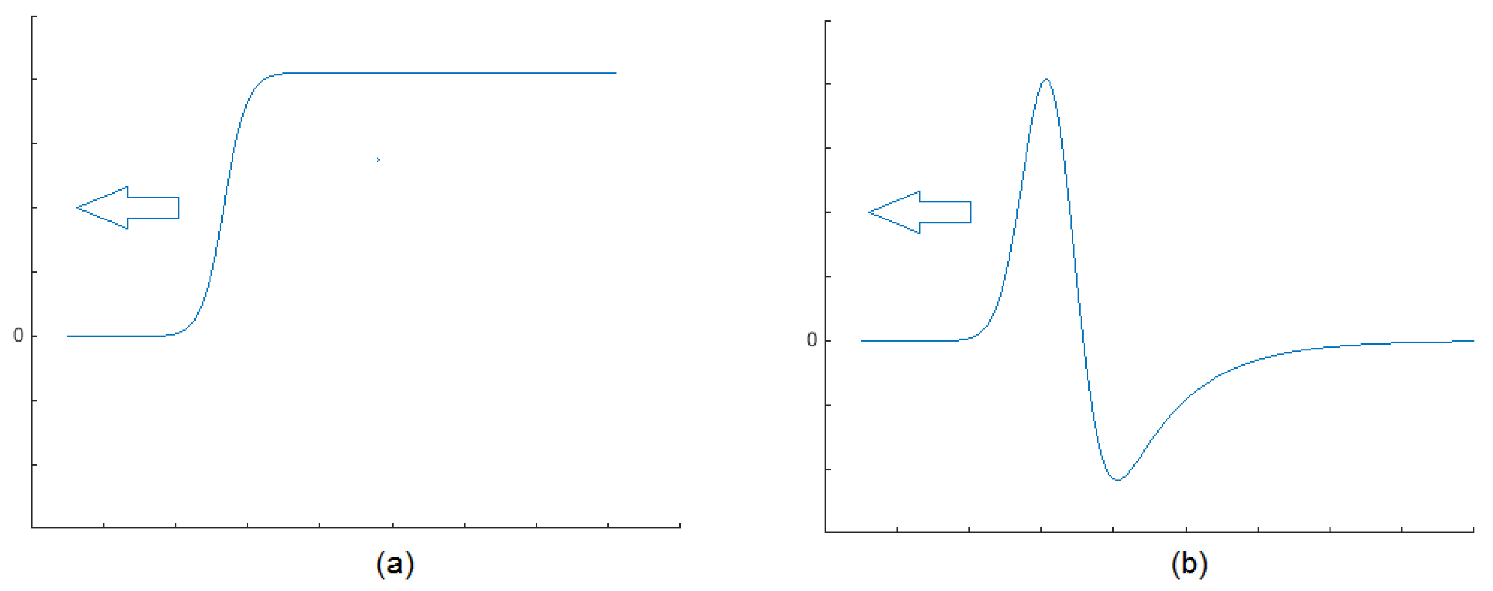
3.1. Problem Setting

Here, we consider the following version of the model (2) rescaled with respect to the time variable and containing a parameterization of the firing rate function as follows:
t u ( t , x ) = u ( t , x ) + R ω ( x y ) f β ( u ( t , y ) ) d y v ( t , x ) , 1 ϵ t v ( t , x ) = u ( t , x ) σ v ( t , x ) , t 0 , x R , σ > 0 , 0 < ϵ 1 .
Here, the steepness of the firing rate function f β is parameterised by β [ 0 , ) .
We impose the following assumptions on the functions involved in (3):
( A 1 ) The connectivity kernel ω C 1 ( R , R ) L ( R , μ , R ) is non-negative.
( A 2 ) For β = 0 , the firing rate function is represented by the Heaviside-type function as follows:
f 0 ( u ) = 0 , u h , 1 , u > h ,
where h > 0 .
( A 3 ) For each β > 0 , f β : R [ 0 , 1 ] is non-decreasing and continuous. Moreover, as shown with β β ^ , the following also apply:
(i)
f β f β ^ uniformly on R for β ^ ( 0 , ) ;
(ii)
For any ε > 0 , f β f β ^ uniformly on R B R ( h , ε ) for β ^ = 0 .
Now, we introduce the definition of “travelling wave” solutions to Equation (3) (or simply travelling waves in the neural field (3)).
Definition 3. 
Let h > 0 be fixed. We say that u C [ 0 , ) , C 0 1 ( R , R ) is a travelling wave with the speed c R , if u ( t , x ) = U ( x c t ) , where the travelling wave profile U C 0 1 ( R , R ) satisfies the following properties:
( B 1 ) U ( x ) > h on ( 0 , a ) R .
( B 2 ) U ( x ) < h on R [ 0 , a ] . If U C 0 1 ( R , R ) , it also satisfies the property.
( B 3 ) U ( 0 ) 0 and U ( a ) 0 , then U is called a regular travelling wave profile, and u is referred to as a regular travelling wave.
Remark 1. 
In Definition 3 and further on, the uniqueness of the ordered pair ( 0 , a ) a > 0 is understood as a modulo translation due to the translation invariance property of U C 0 1 ( R , R ) .
Note that a regular travelling wave profile is stable to small perturbations in C 0 1 ( R , R ) . More precisely, we obtain the following evident result:
Lemma 4. 
Let U ^ C 0 1 ( R , R ) be a regular travelling wave profile. Then, there exists r > 0 such that any U B C 0 1 ( R , R ) ( U ^ , r ) is a regular travelling wave profile.
The remaining part of this section deals with the problem of existence of regular travelling waves in neural fields with continuous and discontinuous firing rate functions and continuous dependence of these solutions on the parameter β .

3.2. Existence and Continuous Dependence of Travelling Wave Profiles on Firing Rate Functions

In this subsection, we prove the main two theorems providing conditions for the existence and continuous dependence of travelling waves profiles on the firing rate function.
If the travelling wave solution to (3) exists, the function U that determines the profile of the travelling wave u ( t , x ) = U ( x c t ) satisfies the following system of equations:
c U ( x ) = U ( x ) + R ω ( x y ) f β ( U ( y ) ) d y V ( x ) , c V ( x ) = ϵ U ( x ) ϵ σ V ( x ) , x R ,
which we conveniently rewrite in the matrix form
U ( x ) V ( x ) = A U ( x ) V ( x ) 1 c ( F β U ) ( x ) 0 , x R ,
where
A = 1 / c 1 / c ϵ / c ϵ σ / c ,
and
( F β U ) ( x ) = R ω ( x y ) f β ( U ( y ) ) d y , x R .
For the travelling wave speed c < 0 , the eigenvalues λ 1 , 2 ,
λ 1 = 1 + ϵ σ 1 ϵ σ 4 ϵ 2 c , λ 2 = 1 + ϵ σ + 1 ϵ σ 4 ϵ 2 c ,
of the matrix A are negative. Thus, there exists a unique bounded solution of the system
ξ ( x ) η ( x ) = A ξ ( x ) η ( x ) 1 c ξ ( x ) 0
in C ( R , R ) × C ( R , R ) , which can be expressed as follows (see, e.g., [39]):
ξ ( x ) η ( x ) = 1 c x exp A ( x y ) ξ ( y ) 0 d y , x R .
In the studies of travelling waves, the decay σ of the negative feedback in the neural medium is often neglected (see, e.g., [16]). Our approach allows us to omit this restriction.
Equation (8) defines a bounded linear operator L : C ( R , R ) C ( R , R ) as a first component of the vector as follows:
( L ξ ) ( x ) = 1 0 , 1 c x exp A ( x y ) ξ ( y ) 0 d y , x R .
where ( · , · ) stands for the dot product.
The system (4) can, thus, be reduced to the following operator equation:
U = H β U ,
H β = L F β ,
where the mappings F β (for each β [ 0 , ) ) and L are defined by (6) and (9), respectively.
To assist the proofs of our main results, we decompose the mapping F β as follows:
F β = W N β ,
where
( W g ) ( x ) = R ω ( x y ) g ( y ) d y , x R ,
( N β g ) ( x ) = f β ( g ( x ) ) , x R .
Lemma 5. 
Let ϵ σ 1 < 0 , c < 0 and the assumptions ( A 1 ) ( A 3 ) be satisfied, then
H β : C 0 1 ( R , R ) C 0 1 ( R , R ) .
Proof. 
Due to the assumptions ( A 2 ) and ( A 3 ) , the operator N β maps any function from C 0 1 ( R , R ) to L ( R , μ , R ) . The operator W defined by (12) is a linear and continuous mapping from L ( R , μ , R ) to C ( R , R ) provided that assumption ( A 1 ) holds true. Next, the operator L given by (9) can be considered as a linear continuous mapping from C ( R , R ) to C 1 ( R , R ) .
Consider ξ C ( R , R ) , ξ ( x ) 0 , for all x R . Using the eigenvalue decomposition of A in (5), we obtain
A = P λ 1 0 0 λ 2 P 1 ,
where λ 1 , 2 are given by (7), and the columns of P are the corresponding eigenvectors of A. Let P = ( p i j ) , i , j = 1 , 2 ; then, L ξ can be rewritten as follows:
( L ξ ) ( x ) = 1 c x k ( x y ; c ) ξ ( y ) d y , k ( x ; c ) = l 2 exp ( λ 2 ( c ) x ) l 1 exp ( λ 1 ( c ) x ) ,
where
l 1 = p 11 p 22 p 11 p 22 p 12 p 21 and l 2 = p 12 p 21 p 11 p 22 p 12 p 21 ,
p 1 j = ( ϵ σ 1 ) ( 1 ) j ( ϵ σ 1 ) 2 4 ϵ 2 ϵ , p 2 j = 1 , j = 1 , 2 .
Thus, we have 0 < l 1 < l 2 , so k ( | x | ; c ) is a typical example of a “wizard hat” function (see Figure 2), which represents a standard way of coupling long-range inhibition and short-range excitation in the neural field models, see, e.g., [10].
Thus, for each non-negative function ξ C ( R , R ) , it is easy to observe the asymptotics as follows:
lim x ( L ξ ) ( x ) = lim x ( L ξ ) ( x ) = + 0 .
Finally, the observation that the function W N β g 0 or any g C ( R , R ) and β [ 0 , ) , under assumptions ( A 1 ) ( A 3 ) , completes the proof. □
Lemma 6. 
Let assumptions ( A 1 ) ( A 3 ) be satisfied, h > 0 , and U ^ C 0 1 ( R , R ) be a regular travelling wave profile. Then, there exists r 0 > 0 such that, for any β [ 0 , ) ,
(i)
H ( · ) ( · ) is continuous on [ 0 , ) × B C 0 1 ( R , R ) ( U ^ , r 0 ) ;
(ii)
The operators { H β : B C 0 1 ( R , R ) ( U ^ , r 0 ) C 0 1 ( R , R ) } β [ 0 , ) are collectively compact.
Proof. 
(i) We start by showing that the operator N β : B C 0 1 ( R , R ) ( U ^ , r ) L ( R , μ , R ) is continuous at any β ^ [ 0 , ) uniformly on B C 0 1 ( R , R ) ( U ^ , r 0 ) .
Let β ^ ( 0 , ) , then assumption ( A 3 ) implies the following:
N β U N β ^ U L ( R , μ , R ) = R | f β ( U ( x ) ) f β ^ ( U ( x ) ) | d x 0 , β β ^ ,
which is uniform with respect to U B C 0 1 ( R , R ) ( U ^ , r 0 ) . For β ^ = 0 , we have
N β U N β ^ U L ( R , μ , R ) = R | f β ( U ( x ) ) f 0 ( U ( x ) ) | d x = = R B R ( h , r 0 ) | f β ( U ( x ) ) f 0 ( U ( x ) ) | d x + B R ( h , r 0 ) | f β ( U ( x ) ) f 0 ( U ( x ) ) | d x .
For x R B R ( h , r 0 ) and any U B C 0 1 ( R , R ) ( U ^ , r 0 ) , the value U ( x ) belongs to R B R ( h , r 0 ) . It follows from ( A 3 ) that the first term on the right-hand side of (14) converges to 0 uniformly on B C 0 1 ( R , R ) ( U ^ , r 0 ) , as β 0 . Next, we estimate the second term as
B R ( h , r 0 ) | f β ( U ( x ) ) f 0 ( U ( x ) ) | d x < 1 c 0 U ^ C 0 1 ( R , R ) U ^ C 0 1 ( R , R ) | f β ( s ) f 0 ( s ) | d s ,
where 0 < const < | U ( x ) | for all x B R ( h , r 0 ) and any U B C 0 1 ( R , R ) ( U ^ , r 0 ) . Here, without the loss of generality, we assume that r 0 < min x B R ( h , r 0 ) | U ^ ( x ) | ). Assumption ( A 3 ) guarantees convergence to 0 of the expression on the right-hand side of the latter inequality, as β 0 .
Next, we utilise the fact that both W : L ( R , μ , R ) C ( R , R ) and L : C ( R , R ) C 0 1 ( R , R ) are linear continuous mappings (see the details in the proof of Lemma 5).
Thus, for any β [ 0 , ) , it holds true that H β : B C 0 1 ( R , R ) ( U ^ , r 0 ) C 0 1 ( R , R ) and
H β U i H β ^ U 0 C 1 ( R , R ) 0 , β β ^ ,
where U 0 B C 0 1 ( R , R ) ( U ^ , r 0 ) , U i U 0 C 0 1 ( R , R ) 0 .
(ii) We notice that due to ( A 1 ) ( A 3 ) , we have W N β : B C 0 1 ( R , R ) ( U ^ , r 0 ) C ( R , R ) , which makes it possible to utilise the Arzela–Ascoli theorem (see, e.g, [40], Section IV.6.7, Theorem 7).
Choose arbitrary ε > 0 . Then, there exist r ε > 0 and β ε > 0 , such that
| R ω ( x y ) f β ( U ( y ) ) d y | < ε
for any U B C 0 1 ( R , R ) ( U ^ , r 0 ) , x R B R ( 0 , r ε ) , and β [ 0 , β ε ) .
Assumptions ( A 1 ) ( A 3 ) imply that the set of functions is bounded and equicontinuous, as shown below:
R ω ( x y ) f β ( U ( y ) ) d y , U B C 0 1 ( R , R ) ( U ^ , r 0 ) , x B R ( 0 , r ε )
According to Arzela–Ascoli theorem, this set possesses an ε -net, i.e., { ς 1 , , ς N } , N < , ς i C ( B R ( 0 , r ε ) , R ) , i = 1 , , N . For the set of functions, we construct an ε -net as follows:
R ω ( x y ) f β ( U ( y ) ) d y , U B C 0 1 ( R , R ) ( U ^ , r 0 ) , x R B R ( 0 , r ε )
For each element of the set { ς 1 , , ς N } , we continuously connect it to zero, so the set of all such continuations forms a finite ε -net for the following set:
R ω ( x y ) f β ( U ( y ) ) d y , U B C 0 1 ( R , R ) ( U ^ , r 0 ) , x R .
Thus, the mappings (compositions) W N β : B C 0 1 ( R , R ) ( U ^ , r 0 ) C ( R , R ) for β 0 are collectively compact. As we proved that the operator L given by (9) is a linear continuous operator from C ( R , R ) to C 0 1 ( R , R ) , we obtain the collective compactness of the operators H β : B C 0 1 ( R , R ) ( U ^ , r 0 ) C 0 1 ( R , R ) . □
Below, we prove the theorem on the continuous dependence of travelling wave profiles (if they exist) on the parameter β . In order to do so, we demonstrate that assumptions ( A 1 ) ( A 3 ) provide collective compactness of the operators H β , β [ 0 , ) , defined by (11) as acting from some subset of C 0 1 ( R , R ) to C 0 1 ( R , R ) .
Theorem 1. 
Let assumptions ( A 1 ) ( A 3 ) be satisfied, h > 0 , and U ^ C 0 1 ( R , R ) be a regular travelling wave profile. If there exist solutions to (10), say U β = H β U β , that belong to B ¯ C 0 1 ( R , R ) ( U ^ , r ) , for some r > 0 and any β ( 0 , 1 ] , then there exists a solution to H 0 U = U , which belongs to { U β } ¯ (and is a regular travelling wave profile). Moreover, if the solution to H 0 U = U , say U 0 , is unique, then U β U 0 C 0 1 ( R , R ) 0 , as β 0 .
Proof. 
From Lemma 6(ii), the operators H β : B ¯ C 0 1 ( R , R ) ( U ^ , r ) C 0 1 ( R , R ) are collectively compact.
Here, we choose r < r 0 to ensure B ¯ C 0 1 ( R , R ) ( U ^ , r ) B ¯ C 0 1 ( R , R ) ( U ^ , r 0 ) (see Lemma 6).
Then, the set is a pre-compact set in C 0 1 ( R , R ) as shown in the following:
{ U β : U β = H β U β , β [ 0 , 1 ] a n d U B ¯ C 0 1 ( R , R ) ( U ^ , r ) }
We considered an arbitrary sequence β n 0 . Then, the subset { U β n } is pre-compact as well. Therefore, there exists convergent subsequences of { U β n } , i.e., { U γ k } U * B ¯ C 0 1 ( R , R ) ( U ^ , r ) , where γ k = β n k . From Lemma 6(i),
U γ k = H γ k U γ k H 0 U = U , a s γ k 0 .
If the solution to H 0 U = U is unique, then { U β n } has only one limit point, that is, U β n U 0 for any β n 0 .
Since U β , U B ¯ C 0 1 ( R , R ) ( U ^ , r ) B C 0 1 ( R , R ) ( U ^ , r 0 ) , then, from Lemma 4, they are regular travelling profiles. □
We are now ready to formulate the theorem that guarantees the existence of travelling wave profiles for β ( 0 , ) given that a travelling wave profile for β = 0 exists and satisfies some properties.
Theorem 2. 
Let assumptions ( A 1 ) ( A 3 ) be satisfied and h > 0 . In addition, we assume that there exists a travelling wave profile U ^ C 0 1 ( R , R ) that satisfies (10) at β = 0 and conditions ( B 1 ) ( B 3 ) , which is unique in a closed ball B ¯ C 0 1 ( R , R ) ( U ^ , r ) for some r > 0 . If
deg ( I H 0 , B C 0 1 ( R , R ) ( U ^ , r ) , 0 ) 0 ,
then, for any β ( 0 , 1 ] , there exists a travelling wave profile U β B C 0 1 ( R , R ) ( U ^ , r 1 ) , r 1 r , satisfying (10).
Proof. 
Consider the operator family { h β } , β [ 0 , 1 ] ,
h β = I H β .
From Definition 1 and Lemma 6(i), h β : B C 0 1 ( R , R ) ( U ^ , r ) C 0 1 ( R , R ) is a homotopy. Moreover, from Lemma 6(ii), { h β } is compact for each β [ 0 , 1 ] .
In order to apply Lemma 2, it is shown that h β ( u ) 0 for any β [ 0 , 1 ] and u B C 0 1 ( R , R ) ( U ^ , r ) .
First, we observe that H 0 u u for any u B C 0 1 ( R , R ) ( U ^ , r ) , due to the uniqueness assumption on U ^ . Assume now that H β u u does not hold for all u B C 0 1 ( R , R ) ( U ^ , r ) . This implies that there is a sequence { u n } u 0 , u n , u 0 B C 0 1 ( R , R ) ( U ^ , r ) .
The collective compactness and continuity of H β : B C 0 1 ( R , R ) ( U ^ , r ) C 0 1 ( R , R ) ( β [ 0 , ) ), see Lemma 6(ii), implies the following two possibilities for any sequence { U β n } B C 0 1 ( R , R ) ( U ^ , r ) ( β n 0 ) of travelling wave profiles satisfying (10):
(1) U β n U ^ C 0 1 ( R , R ) 0 , as β n 0 ;
(2) For some n ^ and any n > n ^ , U β n U ^ C 0 1 ( R , R ) > r 1 (without the loss of generality, we assume here that β n ^ > 1 ).
This proves that ( I H β ) ( U ) 0 for any U B C 0 1 ( R , R ) ( U ^ , r 1 ) and β [ 0 , 1 ] .
Finally, we apply Lemma 3 to the homotopy (15), thus proving the existence of travelling wave profiles satisfying (10) for any β ( 0 , 1 ] . □

3.3. Existence and Continuous Dependence of Travelling Waves on Firing Rate Functions

In this subsection, we derive conditions providing the validity of the previous section’s theorems for the travelling wave profiles, and interpreting these results for the travelling waves help us to obtain the main result of the present research.
In the case of the Heaviside firing rate function, if a travelling wave exists, its profile is given as follows:
U ( x ; a , c ) = 1 c x k ( x y ; c ) ( W ( y a ) W ( y ) ) d y , W ( y ) = 0 y ω ( ξ ) d ξ ,
or, equivalently,
U ( x ; a , c ) = 1 c 0 k ( y ; c ) ( W ( y x ) W ( y x + a ) ) d y , W ( y ) = 0 y ω ( ξ ) d ξ ,
where ( a , c ) are such that
U ( 0 ; a , c ) = 1 c 0 k ( y ; c ) ( W ( y ) W ( y + a ) ) d y = h , U ( a ; a , c ) = 1 c 0 k ( y ; c ) ( W ( y a ) W ( y ) ) d y = h .
The necessary conditions for the existence of travelling wave solutions of the speed c to (3) are naturally understood here as the correspondence between the pair ( c , h ) ( , 0 ) × ( 0 , + ) and the pair ( θ , α ) R 2 such that U ( θ ; α θ , c ) = h and U ( α ; α θ , c ) = h , which determines the wave width α θ . We note that the travelling wave is regular if
0 k ( y ; c ) ( ω ( y ) ω ( y + a ) ) d y 0 , 0 k ( y ; c ) ( ω ( y a ) ω ( y ) ) d y 0 .
In Figure 3, we provide an example of travelling wave profiles U ( x ; a , c ) in the case of the Heaviside limit. Here, we used the Gaussian connectivity function ω ( x ) = 2 / π exp ( x 2 ) , fixed ε = 0.1 , and three choices of σ . The width a and the wave speed c are obtained by solving (17) numerically. The relation between σ and the wave speed c found from (17) agrees with the physiology of the wave electrical processes in the human brain, which is supported by the results of [41], where the impact of inhibition on cortical travelling waves was studied based on experimental MEG data.
Lemma 7. 
Let the following condition be satisfied:
0 k ( y ; c ) ω ( y a ) d y 0 , 0 k ( y ; c ) ω ( y + a ) d y 0 .
Then, ε > 0 such that the travelling wave profile U = U ( · ; a , c ) defined by (17) is a unique solution to (4) in B C 0 1 ( R , R ) ( U , ε ) for β = 0 .
Proof. 
Assessing the derivatives of the expressions U ( θ ; α θ , c ) = h and U ( α ; α θ , c ) = h with respect to the parameters θ and α at the point ( θ , α ) = ( 0 , a ) , we obtain
0 k ( y ; c ) ω ( y a ) d y = 0 , 0 k ( y ; c ) ω ( y + a ) d y = 0 .
Thus, the condition in (19) guarantees the uniqueness of the solution U = U ( · ; a , c ) in B C 0 1 ( R , R ) ( U , ε ) for some ε > 0 . □
We express (16) in the operator form as follows:
U = H 0 U .
According to Lemma 7, the fixed point U = U ( · ; a , c ) of the operator H 0 is unique in B C 0 1 ( R , R ) ( U , ε ) . Thus, H 0 maps B ¯ C 0 1 ( R , R ) ( U , ε ) into some manifold M C 0 1 ( R , R ) ,
M = υ = 1 c 0 k ( y ; c ) ( W ( y x + θ ) W ( y x + α ) ) d y , ( θ , α ) M R 2 ,
where a compact set M is chosen in a such way that it contains the points ( θ ν , α ν ) for all ν B ¯ C 0 1 ( R , R ) ( U , ε ) . We define the mapping ϕ : M M as follows:
ϕ ( θ , α ) = υ ( x ) , υ ( x ) = 1 c 0 k ( y ; c ) ( W ( y x + θ ) W ( y x + α ) ) d y , x R .
Lemma 8. 
The mapping ϕ : M M defined by (20) is a homeomorphism, and the set M is an absolute neighborhood retract provided that any of the relations in (19) holds true.
Proof. 
First, we note that ϕ : M M is subjective by definition. We prove the injectivity of ϕ : M M using the following expressions for the Frechet derivatives of ϕ :
ϕ θ ( θ , α ) = 1 c 0 k ( y ; c ) ω ( y · + θ ) d y ϕ α ( θ , α ) = 1 c 0 k ( y ; c ) ω ( y · + α ) d y
Assuming ϕ θ ( 0 , a ) = 0 , we obtain 0 k ( y ; c ) ω ( y x + θ ) d y = 0 , for all x Ω , which contradicts (19). We, thus, have ϕ θ ( 0 , a ) 0 . In the same manner, we obtain ϕ α ( 0 , a ) 0 , so the mapping ϕ : M M is a homeomorphism. Considering the properties of homeomorphism, the fact that M is an absolute neighborhood retract implies that M = ϕ ( M ) is an absolute neighborhood retract as well. □
We now define
F = H 0 | M B ¯ C 0 1 ( R , R ) ( U , ε ) , F : M B ¯ C 0 1 ( R , R ) ( U , ε ) M .
The mapping F : M B ¯ C 0 1 ( R , R ) ( U , ε ) M is compact and admissible by its definition. Considering the properties of the topological fixed point index, it holds true that
ind ( H 0 , B C 0 1 ( R , R ) ( U , ε ) ) = ind ( F , M B C 0 1 ( R , R ) ( U , ε ) ) .
We apply Lemma 2 and obtain
ind ( F , M B C 0 1 ( R , R ) ( U , ε ) ) = ind ( ϕ 1 F ϕ , ϕ 1 ( F ( M B C 0 1 ( R , R ) ( U , ε ) ) ) .
Lemma 9. 
There exists δ > 0 such that Ψ = ϕ 1 F ϕ maps B ¯ R 2 ( ( 0 , a ) δ ) to M .
Proof. 
Let υ ( x ) = 1 c 0 k ( y ; c ) ( W ( y x + θ ) W ( y x + α ) ) d y , ( θ , α ) M . As assumption ( A 1 ) is fulfilled, for any ε > 0 , one can find δ > 0 such that u U C 0 1 ( R , R ) < ε for all ( θ , α ) B ¯ R 2 ( ( 0 , a ) , δ ) , where U is given by (16). The latter estimate implies that
B ¯ R 2 ( ( 0 , a ) , δ ) ϕ 1 ( M B C 0 1 ( R , R ) ( U , ε ) ) ,
from where we conclude that
M δ F ( M B C 0 1 ( R , R ) ( U , ε ) ) M δ = { υ ( x ) = 1 c 0 k ( y ; c ) ( W ( y · + θ ) W ( y · + α ) ) d y , ( θ , α ) B ¯ R 2 ( ( 0 , a ) , δ ) } .
Thus, we obtain
ϕ 1 ( M δ ) = B ¯ R 2 ( ( 0 , a ) , δ ) ϕ 1 ( F ( M B C 0 1 ( R , R ) ( U , ε ) ) ) ,
and complete the proof. □
Due to the fact that U is an isolated fixed point of F and topological invariance property of the index, ( 0 , a ) is an isolated fixed point of Ψ . Thus, we have
Ψ ( 0 , a ) = Ψ 1 ( 0 , a ) , Ψ 2 ( 0 , a ) , Ψ ( 0 , a ) = 1 c 0 k ( y ; c ) ( W ( y Ψ 1 ( a , b ) ) W ( y Ψ 2 ( a , b ) + α ) ) d y .
The topological index of the mapping Ψ = Ψ 1 ( θ , α ) , Ψ 2 ( θ , α ) for ( θ , α ) = ( 0 , a ) can be found as follows:
ind ( Ψ , ϕ 1 ( F ( M B C 0 1 ( R , R ) ( U , ε ) ) ) = = sgn det ( Ψ 1 ) θ ( 0 , a ) 1 ( Ψ 1 ) α ( 0 , a ) ( Ψ 2 ) θ ( 0 , a ) ( Ψ 2 ) α ( 0 , a ) 1 .
We use the following relations for
( U ( θ ; α θ , c ) ) θ = 0 , ( U ( θ ; α θ , c ) ) α = 0 ,
( U ( α ; α θ , c ) ) θ = 0 , ( U ( α ; α θ , c ) ) α = 0 a t ( θ , α ) = ( 0 , a )
and obtain
( Ψ 1 ) θ ( 0 , a ) = 0 k ( y ; c ) ω ( y ) ω ( y ) ω ( y + a ) d y ; ( Ψ 1 ) α ( 0 , a ) = 0 k ( y ; c ) ω ( y + a ) ω ( y + a ) ω ( y ) d y ;
( Ψ 2 ) θ ( 0 , a ) = 0 k ( y ; c ) ω ( y + a ) ω ( y a ) ω ( y ) d y ; ( Ψ 2 ) α ( 0 , a ) = 0 k ( y ; c ) ω ( y ) ω ( y ) ω ( y a ) d y .
Thus, deg ( I H 0 , B C 0 1 ( R , R ) ( U , ε ) , 0 ) 0 if
( Ψ 1 ) θ ( 0 , a ) ( Ψ 2 ) α ( 0 , a ) ( Ψ 1 ) α ( 0 , a ) ( Ψ 2 ) θ ( 0 , a ) ( Ψ 1 ) θ ( 0 , a ) ( Ψ 2 ) α ( 0 , a ) + 1 0 .
The results above, together with Theorems 1 and 2, imply the main result of the present research.
Theorem 3. 
Let assumptions ( A 1 ) ( A 3 ) be satisfied. Let the condition in (17) be fulfilled and the inequalities of (18), (19), and (21) hold true. Then, for each β [ 0 , ) , there exists a regular travelling wave solution u β C 0 1 ( R , R ) ) of the speed c < 0 to (3). Moreover,
max t [ 0 , ) u β ( t , · ) u 0 ( t , · ) C 0 1 ( R , R ) 0 , a s β 0 ,
where u 0 C 0 1 ( R , R ) ) is the travelling wave (of the width a) corresponding to β = 0 with the profile defined by (16).
We note that Theorem 1 only provides the convergence of the travelling wave profiles U β U 0 C 0 1 ( R , R ) 0 , as β 0 . However, Definition 3 and the metric in C ( [ 0 , ) , C 0 1 ( R , R ) ) imply the convergence (22).
Remark 2. 
The convergence in (22) takes place not only for β 0 but also for any β ^ ( 0 , ) and any β β ^ . This fact follows from Theorem 3.13 in [36].
Finally, we summarise the algorithm of the practical application of the paper results. Given the characteristics of the neural field (namely, the excitatory connections defined by ω , the neuronal activation threshold h, and the negative feedback strength ϵ and decay σ ), one uses condition (17) to verify the existence of the travelling wave of the width a and the speed c. As soon as the inequality of (17) holds true (i.e., the travelling wave is regular), one verifies the inequalities of (19) and (21). If the inequalities occur, then, for any sufficiently steep firing rate function approximating the Heaviside firing rate function with the threshold h, there exists the corresponding travelling wave of the same speed that approaches (in the sense of the relation (22)) the travelling wave corresponding to the Heaviside firing rate function.

4. Conclusions and Further Discussions

This paper fills the gap between the continuous, i.e., real-world, and the discontinuous, i.e., simplified, models of neuronal activation processes in the research on travelling waves. In a nutshell, the main findings of this paper guarantee that it is now possible to straightforwardly extend many features of the simplified model to the corresponding continuous model, which, in most cases, cannot be studied directly. More specifically, we obtained the conditions explaining when smooth, sigmoidal firing rate functions can be conveniently replaced by much simpler Heaviside-type functions so that the solutions of the simplified model converge to those of the real-world model. This problem is well-known to be mathematically challenging, as no general convergence results can be directly applied in this case. As demonstrated in this paper, using a simplified model has both theoretical and numerical advantages, including the possibility of constructive studies of travelling waves in neural fields, resulting in closed-form expressions for them and significant simplifications of their numerical analysis. By doing so, many important characteristics of cortical travelling waves, such as the wave shape and the wave speed, can be linked to the physiological parameters of the neural medium, such as the lengths and the strengths of neuronal connections and the neuronal activation thresholds in the framework of the neural field theory.
An extension of the present research could be a rigorous study on the stability issues of travelling waves based on the assessment of the spectrum of the Frechet derivative of the corresponding Hammerstein integral operator. This method was recently applied to the investigation of the stability of stationary periodic solutions to neural field equations with Heaviside firing rate functions [42]. The key tool of this study was the proof of the fact that the spectrum of the Hammerstein operator agrees up to zero with the spectrum of a block Laurent operator. It would also be of interest to link the stability/instability properties of travelling waves in the Heaviside firing rate case to the corresponding travelling waves properties in the case of sigmoidal neuronal activation. We expect that the assessment of the spectral properties of the corresponding operators can be carried out using the techniques based on the implicit function theorem, which were successfully exploited in [43] in the proof of the continuous dependence of stationary solutions to neural field equations under the transition from smooth firing rate functions to the Heaviside function.
A more physiologically oriented direction for the extension of the present research could be the investigation of brain travelling waves in the framework of Amari models involving the formalization of the functional microstructure of orientation columns in the visual cortex (see, e.g., [44,45]). The most interesting problems here are related to finding connections between the modifications of travelling waves in the primary visual cortex and the properties of the corresponding modifying visual stimuli. Such experimental data-based investigations require computer modelling of travelling waves in the visual cortex, which should rely on mathematically justified numerical approaches.

Author Contributions

Conceptualization, E.B. and A.P.; methodology, A.O. and A.P.; writing—original draft preparation, E.B. and A.O.; writing—review and editing, E.B., A.O. and A.P.; visualization, A.O. All authors have read and agreed to the published version of the manuscript.

Funding

The work of Evgenii Burlakov was supported by the Russian Science Foundation (Project No. 23-11-20020, https://rscf.ru/en/project/23-11-20020/) (accessed on 19 February 2025).

Data Availability Statement

The original contributions presented in the study are included in the article, further inquiries can be directed to the corresponding author.

Conflicts of Interest

The authors declare no conflicts of interest.

Abbreviations

The following abbreviations are used in this manuscript:
e.g.,exempli gratia (for example)
EEGelectroencephalography
MEGmagnetoencephalography

References

  1. Davis, Z.W.; Muller, L.; Trujillo, J.-M.; Sejnowski, T.; Reynolds, J. Spontaneous travelling cortical waves gate perception in awake behaving primates. Nature 2020, 587, 432–436. [Google Scholar] [CrossRef]
  2. Bhattacharya, S.; Brincat, S.L.; Lundqvist, M.; Miller, E.K. Traveling waves in the prefrontal cortex during working memory. PLoS Comput. Biol. 2022, 18, e1009827. [Google Scholar] [CrossRef]
  3. Butler, K.; Cruz, L. Neuronal traveling waves form preferred pathways using synaptic plasticity. Comput. Neurosci. 2024; ahead-of-print. [Google Scholar] [CrossRef] [PubMed]
  4. Magosso, E.; Borra, D. The strength of anticipated distractors shapes EEG alpha and theta oscillations in a Working Memory task. NeuroImage 2024, 300, 120835. [Google Scholar] [CrossRef]
  5. Davis, Z.W.; Benigno, G.B.; Fletterman, C.; Desbordes, T.; Steward, C.; Sejnowski, T.J.; Reynolds, J.H.; Muller, L. Spontaneous traveling waves naturally emerge from horizontal fiber time delays and travel through locally asynchronous-irregular states. Nat. Commun. 2021, 12, 6057. [Google Scholar] [CrossRef] [PubMed]
  6. Koller, D.P.; Schirner, M.; Ritter, P. Human connectome topology directs cortical traveling waves and shapes frequency gradients. Nature Comm. 2024, 15, 3570. [Google Scholar] [CrossRef] [PubMed]
  7. Drukarch, B.; Wilhelmus, M.M.M. Thinking about the action potential: The nerve signal as a window to the physical principles guiding neuronal excitability. Front. Cell. Neurosci. 2023, 17, 1232020. [Google Scholar] [CrossRef] [PubMed]
  8. Rahmouni, L.; Merlini, A.; Pillain, A.; Andriulli, F.P. On the modeling of brain fibers in the EEG forward problem via a new family of wire integral equations. J. Comp. Phys. X 2020, 5, 100048. [Google Scholar] [CrossRef]
  9. Næss, S.; Halnes, G.; Hagen, E.; Hagler, D.J., Jr.; Dale, A.M.; Einevoll, G.T.; Ness, T.V. Biophysically detailed forward modeling of the neural origin of EEG and MEG signals. NeuroImage 2021, 225, 117467. [Google Scholar] [CrossRef] [PubMed]
  10. Byrne, À.; Ross, J.; Nicks, R.; Coombes, S. Mean-field models for EEG/MEG: From oscillations to waves. Brain Topogr. 2021, 15, 36–53. [Google Scholar] [CrossRef] [PubMed]
  11. Das, A.; Myers, J.; Mathur, R.; Shofty, B.; Metzger, B.A.; Bijanki, K.; Wu, C.; Jacobs, J.; Sheth, S.A. Spontaneous neuronal oscillations in the human insula are hierarchically organized traveling waves. eLife 2022, 11, e76702. [Google Scholar] [CrossRef]
  12. Wilson, H.R.; Cowan, J.D. A mathematical theory of the functional dynamics of cortical and thalamic nervous tissue. Kybernetik 1973, 13, 55–80. [Google Scholar] [CrossRef]
  13. Amari, S. Dynamics of pattern formation in lateral-inhibition type neural fields. Biol. Cybern. 1977, 27, 77–87. [Google Scholar] [CrossRef] [PubMed]
  14. Ermentrout, G.B.; McLeod, J. Existence and uniqueness of travelling waves for a neural network. Proc. Royal Soc. Edinb. Sect. A Mathem. 1993, 123, 461–478. [Google Scholar] [CrossRef]
  15. Klimesch, W.; Hanslmayr, S.; Sauseng, P.; Gruber, W.R.; Doppelmayr, M. P1 and traveling alpha waves: Evidence for evoked oscillations. J. Neurophys. 2007, 97, 1311–1318. [Google Scholar] [CrossRef] [PubMed]
  16. Pinto, D.J.; Ermentrout, G.B. Spatially structured activity in synaptically coupled neuronal networks: I. Traveling fronts and pulses. SIAM J. Appl. Math. 2001, 62, 206–225. [Google Scholar] [CrossRef]
  17. Laing, C.R.; Troy, W. Two-bump solutions of Amari-type models of neuronal pattern formation. Phys. D Nonlinear Phenom. 2023, 178, 190–218. [Google Scholar] [CrossRef]
  18. Owen, M.R.; Laing, C.R.; Coombes, S. Bumps and rings in a two-dimensional neural field: Splitting and rotational instabilities. New J. Phys. 2007, 9, 378. [Google Scholar] [CrossRef]
  19. Blomquist, P.; Wyller, J.; Einevoll, G.T. Localized activity patterns in two-population neuronal networks. Phys. D Nonlinear Phenom. 2005, 206, 180–212. [Google Scholar] [CrossRef]
  20. Naoumenko, D.; Gong, P. Complex dynamics of propagating waves in a two-dimensional neural field. Front. Comput. Neurosci. 2019, 13, 50. [Google Scholar] [CrossRef] [PubMed]
  21. Pinto, D.J.; Jackson, R.K.; Wayne, C.E. Existence and stability of traveling pulses in a continuous neuronal network. SIAM J. Appl. Dyn. Syst. 2005, 4, 954–984. [Google Scholar] [CrossRef]
  22. Coombes, S.; Owen, M.R. Evans functions for integral neural field equations with Heaviside firing rate function. SIAM J. Appl. Dyn. Syst. 2004, 3, 574–600. [Google Scholar] [CrossRef]
  23. Meijer, H.G.; Coombes, S. Numerical continuation of travelling waves and pulses in neural fields. BMC Neurosc. 2013, 14, P70. [Google Scholar] [CrossRef]
  24. Zhang, L. Existence, uniqueness, and exponential stability of traveling wave solutions of some integral differential equations arising from neuronal networks. Diff. Int. Eqs. 2003, 16, 513–536. [Google Scholar] [CrossRef]
  25. Folias, S.E. Nonlinear analysis of breathing pulses in a synaptically coupled neural network. SIAM J. Appl. Dyn. Syst. 2011, 10, 744–787. [Google Scholar] [CrossRef]
  26. Sandstede, B. Evans functions and nonlinear stability of traveling waves in neuronal network models. Int. J. Bifurc. Chaos. 2007, 17, 2693–2704. [Google Scholar] [CrossRef]
  27. Zhang, L. How Do Synaptic Coupling and Spatial Temporal Delay Influence Traveling Waves in Nonlinear Nonlocal Neuronal Networks? SIAM J. Appl. Dyn. Syst. 2007, 6, 597–644. [Google Scholar] [CrossRef]
  28. Bressloff, P.C.; Folias, S.E. Front bifurcations in an excitatory neural network. SIAM J. Appl. Math. 2004, 65, 131–151. [Google Scholar] [CrossRef]
  29. Kilpatrick, Z.P.; Folias, S.E.; Bressloff, P.C. Traveling pulses and wave propagation failure in inhomogeneous neural media. SIAM J. Appl. Dyn. Syst. 2008, 7, 161–185. [Google Scholar] [CrossRef]
  30. Nielsen, B.F.; Wyller, J.A. Ill-posed point neuron models. J. Math. Neurosc. 2016, 6, 7. [Google Scholar] [CrossRef] [PubMed]
  31. Burlakov, E. On inclusions arising in neural field modeling. Diff. Eqs. Dynam. Syst. 2021, 29, 765–787. [Google Scholar] [CrossRef]
  32. Potthast, R.; Graben, P.B. Existence and properties of solutions for neural field equations. Math. Methods Appl. Sci. 2010, 8, 935–949. [Google Scholar] [CrossRef]
  33. Burlakov, E.; Verkhlyutov, V.; Ushakov, V. A simple human brain model reproducing evoked MEG based on neural field theory. Stud. Comp. Intell. 2021, 1008, 109–116. [Google Scholar]
  34. Mawhin, J. Leray-Schauder degree: A half century of extensions and applications. Topol. Meth. Nonlinear Anal. 1999, 14, 195–228. [Google Scholar] [CrossRef]
  35. Katok, A.; Hasselblatt, B. Introduction to the Modern Theory of Dynamical Systems; Cambridge University Press: London, UK, 1995; 793p. [Google Scholar]
  36. Oleynik, A.; Ponosov, A.; Wyller, J. On the properties of nonlinear nonlocal operators arising in neural field models. J. Math. Anal. Appl. 2013, 398, 335–351. [Google Scholar] [CrossRef]
  37. Hutson, V.; Pym, J.S.; Cloud, M.J. Applications of Functional Analysis and Operator Theory; Elsevier: Amsterdam, The Netherlands, 2005; 432p. [Google Scholar]
  38. Granas, A. The Leray-Schuder index and the fixed point theory for arbitrary ANRs. Bull. Soc. Math. 1972, 100, 209–228. [Google Scholar]
  39. Coppel, W.A. Dichotomies in Stability Theory; Springer: New York, NY, USA, 1978; 97p. [Google Scholar]
  40. Dunford, N.; Schwartz, J.T. Linear Operators: I. General Theory; John Wiley & Sons: New York, NY, USA, 1958; 872p. [Google Scholar]
  41. Malkov, I.; Burlakov, E.; Verkhlyutov, V.; Ushakov, V. A model of travelling waves in the neural medium with directional variability of inhibitory effects. Stud. Comp. Intell. 2025, 1179, 244–253. [Google Scholar]
  42. Kolodina, K.; Kostrykin, V.; Oleynik, A. Existence and stability of periodic solutions in a neural field equation. Russ. Univ. Rep. Math. 2021, 26, 271–295. [Google Scholar] [CrossRef]
  43. Ponosov, A.; Oleynik, A.; Kostrykin, V.; Sobolev, A. Spatially localized solutions of the Hammerstein equation with sigmoid type of nonlinearity. J. Diff. Eqs. 2016, 261, 5844–5874. [Google Scholar]
  44. Bressloff, P.C.; Carroll, S.R. Laminar neural field model of laterally propagating waves of orientation selectivity. PLoS Comput. Biol. 2015, 11, e1004545. [Google Scholar] [CrossRef] [PubMed]
  45. Burlakov, E.O.; Verkhlyutov, V.M.; Malkov, I.N. On well-posedness of a mathematical model of evoked activity in the primary visual cortex. Russ. Univ. Rep. Math. 2024, 29, 43–50. [Google Scholar]
Figure 1. Travelling front (a) and travelling wave (b) solutions. The arrows indicate a travelling direction of the solution profiles.
Mathematics 13 00701 g001
Figure 2. Example of the kernel k ( | x | ; c ) with c = 0.2 , ϵ = 0.1 , and three choices of σ , σ = 0 , 1 , 2 .
Mathematics 13 00701 g002
Figure 3. The travelling wave profiles U ( x ; a , c ) in the case of the Heaviside firing rate function. Here, we used ω ( x ) = 2 / π exp ( x 2 ) , threshold h = 0.6 (dashed line), ϵ = 0.1 , and three choices of σ , σ = 0 , 1 , 2 . For σ = 0 , we obtained a = 1.14 and the wave speed c = 0.24 ; for σ = 1 and σ = 2 , we have a = 1.04 , c = 0.19 and a = 0.96 , c = 0.13 , respectively. (The calculated values of a and c are rounded off to two decimals).
Mathematics 13 00701 g003
Disclaimer/Publisher’s Note: The statements, opinions and data contained in all publications are solely those of the individual author(s) and contributor(s) and not of MDPI and/or the editor(s). MDPI and/or the editor(s) disclaim responsibility for any injury to people or property resulting from any ideas, methods, instructions or products referred to in the content.

