Abstract
We investigate how novelly generated solutions of the stochastic space-fractional Davey–Stewartson equations are affected by spatial-fractional derivatives and multiplicative Brownian motion (in the Stratonovich sense). These equations model the behavior of weakly nonlinear water waves on a fluid surface. By applying the qualitative theory of planar systems, some new fractional and stochastic solutions are obtained. These solutions gain significance from the application of Davey–Stewartson equations to the theory of turbulence for plasma waves, as they can explain several fascinating physical phenomena. Some solutions are graphically displayed to illustrate the influence of noise strength and fractional derivatives on the obtained solutions. These effects influence the solution’s amplitude and width, as well as its smoothness.
Keywords:
bifurcation theory; wave solutions; modified Riemann–Liouville derivative; stochastic fractional differential equations; nonlinear water waves MSC:
32W50; 35B32
1. Introduction
Alfred Davey and Keith Stewartson first proposed the Davey–Stewartson equations (DSEs) in 1974. Their system of coupled partial differential equations characterizes the behavior of weakly nonlinear water waves on a fluid surface [1]. It has the form [1]
where is a complex field representing the wave amplitude, and is a real field characterizing the interaction of the velocity potential of the mean flow with the surface wave. System (1) has two main versions, DS-I and DS-II, differing in the constant coefficient a, which influences the interactions between wave components [2]. Equation (1) simplifies to the DS-I equation when and to the DS-II equation when . Both DS-I and DS-II have two space dimensions and an integrable equation that appears to generalize the nonlinear Shrödinger equation [1]. The Davey–Stewartson equations can also be reduced to Hamiltonian ODEs, allowing for analytic solutions through the integrability of finite-dimensional Hamiltonian systems [3]. Nonlinear wave phenomena have been reported in numerous scientific and engineering fields, including chemical physics, solid-state physics, biology, plasma physics, optical fibers, fluid mechanics, and geology. Dispersion, dissipation, diffusion, reaction, and convection are key components of nonlinear wave equations. Thus, we find great interest in the wave phenomena literature. Some periodic and solitary solutions of Equation (1) were obtained using the sine–cosine method [4]. In [5], the authors applied the method to solve Equation (1), a work which was extended in [6], where the authors employed the generalized method. The simplest equation method was applied to construct a multiple-soliton solution for Equation (1). The improved and generalized expansion methods were employed to construct solutions for Equation (1), classified into soliton, kink, periodic, and rational solutions in [7]. In [8], the authors employed the generalized Jacobi elliptic expansion method to construct periodic and optical soliton solutions for Equation (1). In [9], a solitary solution, dark solitan, and singular wave were obtained using the trail equation method and ansatz approach. Some solutions for Equation (1) were also derived using the first integral method [10]. In [11], the author studied a (2+1)-dimensional generalized modified dispersive water–wave system and constructed a hetero-Bäcklund transformation, bilinear forms, and soliton solutions. In [12], the author established several bilinear auto-Bäcklund transformations and similarity reductions in a (2+1)-dimensional generalized nonlinear evolution system in fluid dynamics, plasma physics, nonlinear optics, and quantum mechanics, which are a key areas of research in both science and engineering. Moreover, an extended time-dependent (3+1)-dimensional shallow-water wave equation, relevant to ocean and river dynamics, was analyzed using symbolic computation to derive a set of bilinear auto-Bäcklund and similarity transformations [13]. Additionally, in [14], the author investigated a (3+1)-dimensional Korteweg–de Vries–Calogero–Bogoyavlensky–Schiff equation with time-dependent coefficients for shallow-water waves, constructing solutions using the method and method and applying the simplified Hirota method to derive soliton solutions.
Fractional calculus provides a useful description for many natural phenomena. It has been used in a variety of applications including the study of image processing, electromagnetic phenomena, acoustic phenomena, anomalous diffusion, and electrochemical processes, see, e.g., [15,16,17,18].
Numerous disciplines, including engineering, climate dynamics, chemistry, physics, geophysics, atmospheric sciences, biology, and fluid mechanics, have incorporated random effects into the statistical analysis, simulation, prediction, and modeling of complex systems [19,20,21,22,23,24,25]. Noise cannot be disregarded, as it can trigger some intriguing phenomena [26]. Solving the fractional partial differential equations (PDEs) with stochastic components is generally more difficult than solving the so-called traditional PDEs [27].
In the current paper, we consider the stochastic space-fractional Davey–Stewartson equations, which describe the behavior of weakly nonlinear water waves at a fluid’s surface. These equations take the following form:
where is the noise strength, is a Brownian motion, and is the Jumarie’s modified Riemann–Liouville fractional derivative of order q. To make the paper self-contained, we have added Appendix A containing the needed results about the modified Riemann–Liouville fractional derivative and Brownian motion. It is understood that the stochastic integral, , can be interpreted in several different ways, often as Stratonovich and Itô calculus [28]. A Stratonovich stochastic integral (denoted as ) is evaluated at the midpoint, while an Itô stochastic integral (denoted as ) is computed at the left endpoint when it is investigated at the left endpoint. Stratonovich calculus is preferred in real-world applications because it accurately represents multiplicative noise influenced by past values, ensuring greater consistency with experimental observations [27]. Both integrals are related by the following equation:
when Y possesses sufficient regularity, where represents a stochastic process. The stochastic system (2) has been studied in several works, both with fractional- and integer-order derivatives. In particular, System (2), with a conformable fractional derivative, was investigated in [29], where the authors employed the Riccati–Bernoulli sub-ordinary differential equation and the sine–cosine method to derive solutions classified as hyperbolic, trigonometric, and rational stochastic solutions. It was also examined in [30], where the authors utilized the improved modified extended tanh-function method to construct soliton solutions and investigate its chaotic behavior. For the case of integer-order derivatives (i.e., when q approaches 1), system (2) has been explored in several works. In [31], the authors constructed soliton, kink, periodic, and rational solutions using the method and analyzed its chaotic behavior through sensitivity analysis. In [32], the mapping method was employed to obtain new rational, elliptic, hyperbolic, and trigonometric solutions. Additionally, in [33], the Sardar subequation method was applied to derive stochastic optical soliton solutions, including dark, bright, combined, and periodic waves. Lastly, in [34], the complete discriminant polynomial system was utilized to construct various solutions.
To the best of our knowledge, space-fractional stochastic Davey–Stewartson equations have been studied in only a few works, all of which focused on conformable fractional derivatives, which are local. This motivated us to use Jumarie’s modified Riemann–Liouville fractional derivative, which is more relevant for real-world applications due to its nonlocal nature (see, e.g., [35]), and to apply bifurcation analysis to construct fractional stochastic solutions.
The objective of this work is to derive analytical solutions for the fractional Davey–Stewartson equations (2) using the qualitative theory of planar integrable systems. Specifically, we analyze how the model’s solutions evolve as a certain parameter, known as the bifurcation parameter, varies. Furthermore, we explore the individual and combined effects of the fractional order and noise strength on the obtained solutions, providing numerical illustrations using Mathematica 14 software.
This work is structured as follows: Section 2 presents an analysis that transforms the system (2) into a dynamical system. Section 3 provides a qualitative analysis of the reduced dynamical system and studies the phase portrait. Section 4 introduces some new solutions, and includes graphical representations of these solutions to illustrate the impact of noise strength and fractional order. Finally, Section 6 summarizes the main results.
2. Mathematical Analysis
We assume that the solution to system (2) has the form
with
where are free constants. Utilizing Jumarie’s modified Riemann–Liouville fractional derivative of order q, we derive the following formulas:
Substituting the expressions (6) into Equation (1a), we obtain the real part and the imaginary part.
The real part:
The imaginary part:
Equation (8) holds identically if
Substituting the expressions (6) into Equation (2b), we obtain
which is integrated twice with respect to , neglecting the constants of integration. This yields
Since is the standard normal process, we have , where is the expectation. Taking the expectation of both sides of Equation (12), we obtain, after some simplification,
where are new constants introduced to simplify the expression and are given by
Equation (13) is written in the form
The system (15) is conservative because . The Hamiltonian canonical equations, with a Hamiltonian function in the form
give system (15), and, consequently, it is a Hamiltonian system [36,37]. Based on the Hamiltonian function (16), which does not rely on the independent variable (acting as time in Hamiltonian mechanics), it remains constant along all the phase orbits of the system (15), i.e.,
where is a constant that will be determined later from the initial conditions. The expression on the left-hand side of (17) is a conserved quantity. The Hamiltonian function (16) models the 1D motion of a particle governed by a two-parameter potential function.
Thus, the issue of solving Equation (2) is reduced to finding a solution for the particle’s one-dimensional motion, which can be solved by quadrature as it is completely integrable. Inserting the first equation of Equation (15) into the conserved quantity and separating the variables, we obtain the one-dimensional differential form as
where is a quartic polynomial and admits the form
The range of the parameters , and r is a demand for integrating the differential form (19). It can be evaluated by employing different two methods. They are bifurcation analysis [38], which was applied successfully in several papers such as [25,39,40], and the complete discriminate polynomial system [41]. Bifurcation analysis has been effectively utilized in various studies, including [39,42,43,44], and will be used in this work.
3. Analysis of Bifurcation
In this section, the bifurcation of the Hamiltonian system (18) is analyzed using Hamiltonian concepts, which are introduced briefly in Appendix B, with a detailed description of its phase portrait.
The equilibrium points of the system (18) correspond to the critical points of the potential function (18). Consequently, these points are given by , where is a solution of . If , the system (18) has a single equilibrium point, . However, if , it has, in addition to O, two additional equilibrium points, . The nature of these points—whether they are a maximum (saddle point) or a minimum (center point) of the potential function (18)—is determined as in [37]. We have
Thus, using the above computations, we obtain the following:
- (a)
- If (), the unique equilibrium point O is a maximum of the potential function (18) and, therefore, a saddle point. Conversely, if (), it is a minimum of the potential function (18) and thus a center. See Figure 1a,b for a visualization, and Figure 2 for the corresponding phase portrait.
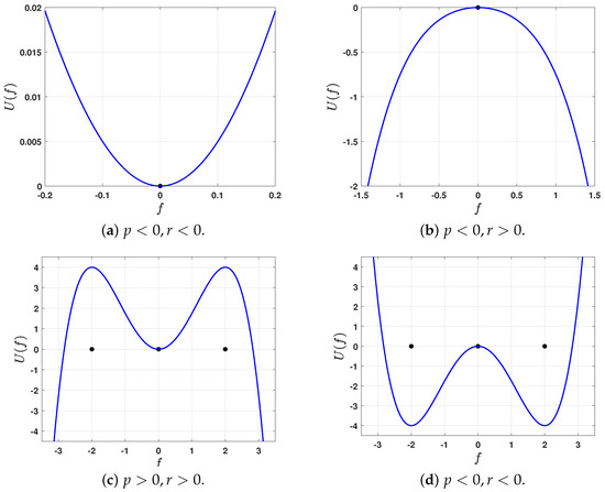 Figure 1. The graph for the potential function (18) for distinct values of p and r. The black solid point indicates the equilibrium point.
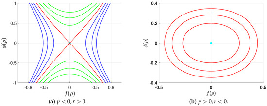 Figure 2. The phase portrait of the system (15) for , where the cyan point marks the equilibrium point.
 - (b)
- When (), O is a maximum of the potential function (18) and is therefore a saddle point, while are minima and thus serve as center points. Conversely, when (), O becomes a minimum of the potential function (18), making it a center, whereas are maxima and therefore saddle points. See Figure 1c,d for visualization. The corresponding phase portraits are shown in Figure 3.
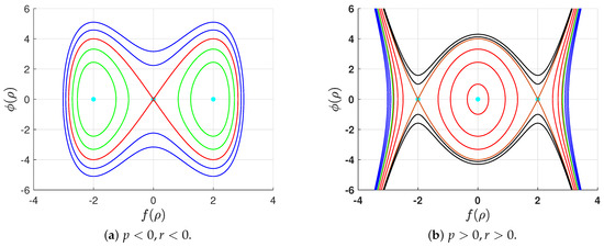 Figure 3. The phase portrait of the system (15) for , where the cyan point marks the equilibrium point.
This proves the following theorem:
Theorem 1.
To determine the geometry of the phase portrait, we need to assess the possible values of at the equilibrium points. Thus, we have
Phase Portrait Description
This subsection aims to describe the phase portrait based on the values of the two parameters p and r and, consequently, .
- (a)
- (b)
- (c)
- For , the system (15) has three equilibrium points, with O being a saddle point and center points. All phase plane orbits are bounded for all values of the parameter , as shown in Figure 3a. The system (15) has a homoclinic orbit in red, two families of periodic orbits in green, and a family of super periodic orbits in blue for , , and , respectively.
- (d)
- When , there are three equilibrium points for the system (15), with O being a center point and saddle points, as displayed by Figure 3b. If , the system has a heteroclinic orbit, shown in brown, connecting the two saddle points , along with its unbounded extension. For , there are three families of orbits in red: one periodic family located inside the heteroclinic orbit, and two unbounded families located outside the heteroclinic orbit. The system has two families of unbounded orbits in black when in addition to a green orbit when . For , there are two families of unbounded orbits in blue.
4. Solutions
This section aims to apply the bifurcation constraints on the parameters introduced in Section 3 to construct solutions for Equation (2). We exclude unbounded orbits from our consideration, as they have less physical significance.
- (a)
- When , the polynomial (20) has two real roots, , and two purely imaginary roots, . Thus, it takes the form . The interval of real solutions for is . By taking and integrating both sides of Equation (19), we obtainwhere is a Jacobi elliptic function [45]. Thus, the solution of Equation (2) becomeswhere is the incomplete elliptic integral of the second kind, defined aswhere u and k represent the amplitude and elliptic modulus, respectively, with for real applications. For further details on Jacobi elliptic functions, see, e.g., [45]. Solution (24) represents a novel solution to Equation (2).
- (b)
- For , we construct different types of solutions based on the various values of .
- i.
- For positive values of , the system (15) exhibits a family of super periodic orbits, shown in blue in Figure 3a. A single orbit from this family intersects the axis at two points. Therefore, the polynomial (20) has two real roots, , and two purely imaginary roots, , and thus has the form . By taking , and integrating both sides of Equation (19), we obtainwhere denotes the Jacobi elliptic function [45]. Employing Equations (4) and (11), a solution to Equation (2) is found in the formThis expression gives a new solution for Equation (2).
- ii.
- At the zero level of the parameter , there is a homoclinic orbit in red for the system (15), as displayed by Figure 3a. This indicates that the polynomial has a double root at the origin and two simple roots at . Thus, we have . Taking and integrating both sides of Equation (19), we obtainEquation (29) provides a novel solution to Equation (2).
- iii.
- At a fixed value for the parameter , the system has two families of periodic orbits, as shown in green in Figure 3a. In this case, the polynomial (20) has four real roots, and , where , and, hence, it has the form . The function is real when . Let . Integration of both sides of Equation (19) provideswhere is a Jacobi elliptic function [45]. A new solution to Equation (2) is found by utilizing both Equations (4) and (11). Therefore, we have
- (c)
- When , the solutions of Equation (2) depend on the values of .
- i.
- For , any orbit of the system (15) intersects the axis at four points, as shown in red in Figure 3b. This means that the polynomial (20) has four real roots, and . Therefore, it can be written as , where . The function is real and bounded in the interval . By taking and integrating both sides of Equation (19), we obtain
- ii.
- On the level , the system (15) has a heteroclinic orbit, as shown in brown in Figure 3b. This indicates that the polynomial has two double roots which are the coordinates for the saddle points . Hence, takes the form . The function is real if . Taking and integrating both sides of Equation (19), we obtain
It is worth mentioning that all previous works have utilized conformable fractional derivatives or beta fractional derivatives, which are local in nature. In our study, we use Jumarie’s modified Riemann–Liouville fractional derivative for the first time. This derivative is more relevant for real-world applications due to its nonlocal properties [35]. Consequently, all the obtained solutions are entirely new.
5. Physical Interpretation
The fractional order impact, noise strength influence, and their combination on the solutions are explored in this section. We focus on studying these impacts on , and similarly for .
Let us choose . Then, we have , , and . Since , and selecting , the expression (24) is a solution to Equation (2), which has the form
The fractional order impact and noise strength separately influence the solution (24) to Equation (2), which will now be discussed.
The noise strength impact on the solution (24) to Equation (2) with integer-order derivatives, i.e., when , is shown in Figure 4. Figure 4a shows that the solution (24) is periodic in the deterministic case and is not symmetric about the vertical axis. The solution amplitude increases with increasing noise strength, while the solution width remains relatively constant. The surface, which highlights the solution (24), is smooth in the deterministic case, but it becomes rough as the noise strength grows, as shown in Figure 4b.
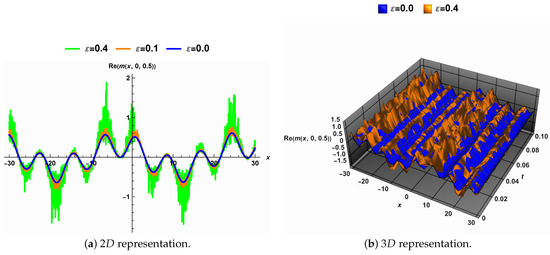
Figure 4.
The noise strength impact on the solution (24) when .
Figure 5 explains the fractional-order derivatives’ impact on the solution in the deterministic case, i.e., when . Figure 5a illustrates how the solution width greatly rises as the fractional order q drops from one. The surface described by the solution (24) is smooth for all fractional order values q, as Figure 5b demonstrates.
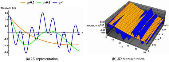
Figure 5.
The impact of fractional order q on the solution (24) in the deterministic case, i.e., .
Figure 6 highlights the joint noise strength and the fractional derivative order effects on the solution (24). Figure 6a shows that the solution is periodic in the traditional case, i.e., when and , as shown in blue. However, when the fractional order drops from one and the noise strength grows, the solution’s width grows significantly, causing the solution to lose its periodicity. Furthermore, the surface characterized by the solution (24) becomes rough.
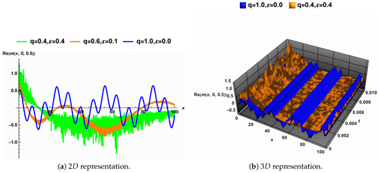
Figure 6.
The combined impact of the fractional-order derivative q and the noise strength on the solution (24).
Let us assume . Then, we have , , and . The phase diagram for the system (15) is highlighted in Figure 3a. By selecting , Equation (2) has the solution (29), which admits the form
Figure 7 depicts the noise strength impact on the solution (29). In Figure 7a, the solution is shown to resemble a solitary solution in the deterministic case, highlighted in blue. To increase the noise strength, the solution’s amplitude grows, while its width remains nearly unchanged. Figure 7b shows that the surface corresponding to the solution (29) becomes rougher with increasing noise strength.
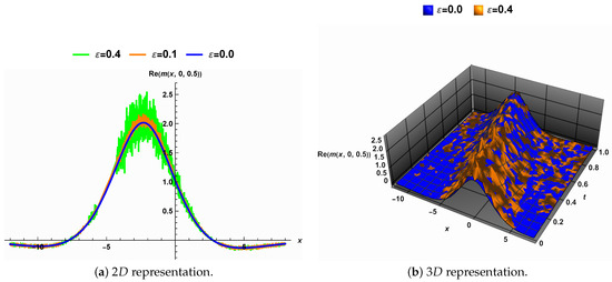
Figure 7.
The noise strength impact on the solution (29) when .
The fractional derivative order impact on the solution (29) is demonstrated in Figure 8. Figure 8a shows that the solution is symmetric when the derivative order is an integer, i.e., , and its symmetry is lost as the fractional order drops from 1. The surface characterized by the solution (29) remains smooth for all values of q, as shown by Figure 8b.
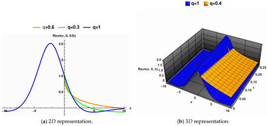
Figure 8.
The order fractional derivative q’s impact on the solution (29) in the deterministic case, i.e., .
The joint impacts of noise strength and fractional order on the solution (29) are displayed in Figure 9. As shown in Figure 9a, the solution is symmetric when , but its symmetry disappears as the fractional order drops from one and the noise strength rises from zero. Additionally, the surface characterizing the solution (29) becomes rough as the noise strength increases and loses its symmetry when the fractional order decreases from one.
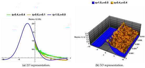
Figure 9.
The joint impact of the order fractional derivative q and the noise strength on the solution (29).
6. Conclusions
This study investigates space-fractional derivatives and multiplicative Brownian motion in the Stratonovich sense, as applied to the stochastic space-fractional Davey–Stewartson equations, which model weakly nonlinear water waves at a fluid’s surface. Transformations were employed to simplify the system into an ordinary differential equation that is equivalent to a Hamiltonian system describing a one-dimensional particle’s motion. The bifurcation method was utilized to analyze this system, and the resulting phase portrait was thoroughly examined. New solutions for the fractional stochastic model (2) were discovered. These solutions are innovative for both the deterministic fractional version of model (2) and the stochastic model with integer derivatives. We used Mathematica to generate 2D and 3D visualizations of these solutions, highlighting the effects of noise strength, fractional-order derivatives, and their interactions. The impact of these factors is reflected in the amplitude, width, and smoothness of the solution surface. Additionally, the impact of noise on the solutions reveals that increased noise disrupts solution patterns, leading to more planar surfaces, which suggests a stabilizing effect. Higher noise intensities drive the analytic solutions toward zero. Moreover, for fixed noise levels, increasing the fractional order q enhances and amplifies the noise. Therefore, understanding the role of q is crucial when analyzing the dynamics of such phenomena. Consequently, selecting an appropriate fractional order q is essential for effectively studying stochastic systems that describe nonlinear water waves.
Author Contributions
Conceptualization, A.E. and M.M.E.-D.; methodology, A.E., M.A.N. and M.M.E.-D.; software, M.A.N.; validation, A.E., M.A.N. and M.M.E.-D.; formal analysis, M.A.N. and M.M.E.-D.; investigation, M.A.N. and M.M.E.-D.; writing—original draft preparation, A.E. and M.M.E.-D.; writing—review and editing, M.A.N.; visualization, A.E.; project administration, A.E. and M.M.E.-D.; funding acquisition, A.E. and M.A.N. All authors have read and agreed to the published version of the manuscript.
Funding
This work was supported by the Deanship of Scientific Research, Vice Presidency for Graduate Studies and Scientific Research, King Faisal University, Saudi Arabia [Grant no. KFU250264].
Data Availability Statement
No data were used to support the study.
Conflicts of Interest
The authors declare no conflicts of interest.
Appendix A. Riemann–Liouville Fractional Derivative Modified by Jumarie and the Standard Wiener Process
Definition A1
([46]). Let for the fractional derivatives of order q in the sense of the Riemann–Liouville fractional derivative modified by Jumarie to the function g, where is defined by
The Riemann–Liouville fractional derivative modified by Jumarie possesses the following properties, which are beneficial in the current work. For additional properties, see, e.g., [46].
- (a)
- , where .
- (b)
- for any differentiable function g at x, in the sense of Jumarie’s modified Riemann–Liouville form.
Definition A2
([28]). A standard Wiener process (or standard Brownian motion) is a stochastic process that satisfies the following properties (Gaussian Increments):
- (a)
- (Initial Condition):;
- (b)
- (Continuity): is a continuous function for ;
- (c)
- (Independent Increments):For , and are independent;
- (d)
- (Independent Increments):
Appendix B. Hamiltonian Concepts
To accomplish our objective, we apply some Hamiltonian concepts. To ensure the article is self-contained, we first introduce some fundamental concepts related to Hamiltonian systems. The 2D dynamical system of the form
is named a Hamiltonian system if there is a function H, which is called a Hamiltonian function, such that [37]
The system (A3) is called canonical Hamiltonian equations and represent the generalized coordinate and generalized angular momentum.
Definition A3
([37]). The dynamical system (A2) is conservative if .
It is obvious from Definition A3 that the Hamiltonian system (A3) is conservative because
The 1D nature of the Hamiltonian system is always written in the form
where is the potential function. The equilibrium points are always the critical points for the potential function. These equilibrium points are classified according to the following Lagrange Theorem:
Theorem A1
(Lagrange Theorem [47]). For a conservative system, if the potential energy has a strict minimum at some positions, then these positions are the positions of stable equilibrium points.
Thus, the equilibrium point is either stable (center) or unstable (saddle) if it is a minimum or maximum point for the potential function.
References
- Davey, A.; Stewartson, K. On three-dimensional packets of surface waves. Proc. R. Soc. London. A. Math. Phys. Sci. 1974, 338, 101–110. [Google Scholar]
- Freeman, N.; Davey, A. On the evolution of packets of long surface waves. Proc. R. Soc. London. A. Math. Phys. Sci. 1975, 344, 427–433. [Google Scholar]
- Zhou, Z.; Ma, W.X.; Zhou, R. Finite-dimensional integrable systems associated with the Davey-Stewartson I equation. Nonlinearity 2001, 14, 701. [Google Scholar] [CrossRef]
- Zedan, H.A.; Monaquel, S.J. The sine-cosine method for the Davey-Stewartson equations. Appl. Math. E-Notes 2010, 10, 103–111. [Google Scholar]
- Ebadi, G.; Biswas, A. The G′/G method and 1-soliton solution of the Davey–Stewartson equation. Math. Comput. Model. 2011, 53, 694–698. [Google Scholar] [CrossRef]
- Abdelaziz, M.A.; Moussa, A.; Alrahal, D. Exact Solutions for the Nonlinear (2+1)-Dimensional Davey-Stewartson Equation Using the Generalized (G′G)-Expansion Method. J. Math. Res. 2014, 6, 91–99. [Google Scholar] [CrossRef][Green Version]
- Aghdaei, M.F.; Manafian, J. Optical soliton wave solutions to the resonant Davey–Stewartson system. Opt. Quantum Electron. 2016, 48, 1–33. [Google Scholar] [CrossRef]
- Gaballah, M.; El-Shiekh, R.M.; Akinyemi, L.; Rezazadeh, H. Novel periodic and optical soliton solutions for Davey–Stewartson system by generalized Jacobi elliptic expansion method. Int. J. Nonlinear Sci. Numer. Simul. 2024, 24, 2889–2897. [Google Scholar] [CrossRef]
- Mirzazadeh, M. Soliton solutions of Davey–Stewartson equation by trial equation method and ansatz approach. Nonlinear Dyn. 2015, 82, 1775–1780. [Google Scholar] [CrossRef]
- Jafari, H.; Sooraki, A.; Talebi, Y.; Biswas, A. The first integral method and traveling wave solutions to Davey–Stewartson equation. Nonlinear Anal. Model. Control 2012, 17, 182–193. [Google Scholar] [CrossRef]
- Gao, X.Y. Hetero-Bäcklund transformation, bilinear forms and multi-solitons for a (2+1)-dimensional generalized modified dispersive water-wave system for the shallow water. Chin. J. Phys. 2024, 92, 1233–1239. [Google Scholar] [CrossRef]
- Gao, X.Y. Symbolic computation on a (2+1)-dimensional generalized nonlinear evolution system in fluid dynamics, plasma physics, nonlinear optics and quantum mechanics. Qual. Theory Dyn. Syst. 2024, 23, 202. [Google Scholar] [CrossRef]
- Gao, X.Y. In an ocean or a river: Bilinear auto-Bäcklund transformations and similarity reductions on an extended time-dependent (3+1)-dimensional shallow water wave equation. China Ocean Eng. 2025. [Google Scholar] [CrossRef]
- Shan, H.W.; Tian, B.; Cheng, C.D.; Gao, X.T.; Chen, Y.Q.; Liu, H.D. N-soliton and other analytic solutions for a (3+1)-dimensional Korteweg–de Vries–Calogero–Bogoyavlenskii–Schiff equation with the time-dependent coefficients for the shallow water waves. Qual. Theory Dyn. Syst. 2024, 23, 267. [Google Scholar] [CrossRef]
- Mohammed, W.W.; Iqbal, N.; Botmart, T. Additive noise effects on the stabilization of fractional-space diffusion equation solutions. Mathematics 2022, 10, 130. [Google Scholar] [CrossRef]
- Yuste, S.B.; Lindenberg, K. Subdiffusion-limited A+ A reactions. Phys. Rev. Lett. 2001, 87, 118301. [Google Scholar] [CrossRef] [PubMed]
- Mohammed, W.W. Fast-diffusion limit for reaction–diffusion equations with degenerate multiplicative and additive noise. J. Dyn. Differ. Equa. 2021, 33, 577–592. [Google Scholar] [CrossRef]
- Peter, O.J.; Oguntolu, F.A.; Ojo, M.M.; Olayinka Oyeniyi, A.; Jan, R.; Khan, I. Fractional order mathematical model of monkeypox transmission dynamics. Phys. Scr. 2022, 97, 084005. [Google Scholar] [CrossRef]
- Weinan, E.; Li, X.; Vanden-Eijnden, E. Some Recent Progress in Multiscale Modeling. In Proceedings of the Multiscale Modelling and Simulation, Lecture Notes in Computational Science and Engineering; Springer: Berlin/Heidelberg, Germany, 2004; Volume 39, pp. 3–21. [Google Scholar]
- Franzke, C.L.; O’Kane, T.J.; Berner, J.; Williams, P.D.; Lucarini, V. Stochastic climate theory and modeling. Wiley Interdiscip. Rev. Clim. Chang. 2015, 6, 63–78. [Google Scholar] [CrossRef]
- Jan, R.; Boulaaras, S. Analysis of fractional-order dynamics of dengue infection with non-linear incidence functions. Trans. Inst. Meas. Control 2022, 44, 2630–2641. [Google Scholar] [CrossRef]
- Boulaaras, S.; Jan, R.; Khan, A.; Ahsan, M. Dynamical analysis of the transmission of dengue fever via Caputo-Fabrizio fractional derivative. Chaos Solitons Fractals X 2022, 8, 100072. [Google Scholar] [CrossRef]
- Elbrolosy, M.; Alhamud, M.; Elmandouh, A. Analytical solutions to the fractional stochastic (3+1) equation of fluids with gas bubbles using an extended auxiliary function method. Alex. Eng. J. 2024, 92, 254–266. [Google Scholar] [CrossRef]
- Almutairi, B.; Al Nuwairan, M.; Aldhafeeri, A. Exploring the Exact Solution of the Space-Fractional Stochastic Regularized Long Wave Equation: A Bifurcation Approach. Fractal Fract. 2024, 8, 298. [Google Scholar] [CrossRef]
- Elbrolosy, M. Qualitative analysis and new exact solutions for the extended space-fractional stochastic (3+1)-dimensional Zakharov-Kuznetsov equation. Phys. Scr. 2024, 99, 075225. [Google Scholar] [CrossRef]
- Horsthemke, W.; Lefever, R. Noise-Induced Transitions in Physics, Chemistry, and Biology; Springer: Berlin/Heidelberg, Germany, 1984. [Google Scholar]
- Oksendal, B. Stochastic Differential Equations: An Introduction with Applications; Springer Science & Business Media: Berlin/Heidelberg, Germany, 2013. [Google Scholar]
- Platen, E.; Bruti-Liberati, N. Numerical Solution of Stochastic Differential Equations with Jumps in Finance; Springer Science & Business Media: Berlin/Heidelberg, Germany, 2010. [Google Scholar]
- Mohammed, W.W.; Al-Askar, F.M.; El-Morshedy, M. Impacts of Brownian motion and fractional derivative on the solutions of the stochastic fractional Davey-Stewartson equations. Demonstr. Math. 2023, 56, 20220233. [Google Scholar] [CrossRef]
- Qi, J.; Cui, Q.; Bai, L.; Sun, Y. Investigating exact solutions, sensitivity, and chaotic behavior of multi-fractional order stochastic Davey–Sewartson equations for hydrodynamics research applications. Chaos, Solitons Fractals 2024, 180, 114491. [Google Scholar] [CrossRef]
- Tariq, M.M.; Riaz, M.B.; Kozubek, T.; Aziz-ur Rehman, M. Exploring chaos and stability: Dynamic insights into the stochastic Davey-Stewartson system through advanced sensitivity analysis. Model. Earth Syst. Environ. 2025, 11, 83. [Google Scholar] [CrossRef]
- Al-Askar, F.M.; Cesarano, C.; Mohammed, W.W. Multiplicative Brownian motion stabilizes the exact stochastic solutions of the Davey–Stewartson equations. Symmetry 2022, 14, 2176. [Google Scholar] [CrossRef]
- Iqbal, M.S.; Inc, M. Optical Soliton solutions for stochastic Davey–Stewartson equation under the effect of noise. Opt. Quantum Electron. 2024, 56, 1148. [Google Scholar] [CrossRef]
- Liu, C.; Li, Z. Multiplicative brownian motion stabilizes traveling wave solutions and dynamical behavior analysis of the stochastic Davey–Stewartson equations. Results Phys. 2023, 53, 106941. [Google Scholar] [CrossRef]
- Kilbas, A.A.; Srivastava, H.M.; Trujillo, J.J. Theory and Applications of Fractional Differential Equations; Elsevier: Amsterdam, The Netherlands, 2006; Volume 204. [Google Scholar]
- Saha, A.; Banerjee, S. Dynamical Systems and Nonlinear Waves in Plasmas; CRC Press: Boca Raton, FL, USA, 2021; p. x+207. [Google Scholar]
- Goldstein, H. Classical Mechanics Addison-Wesley Series in Physics; Addison-Wesley: Reading, MA, USA, 1980. [Google Scholar]
- Nemytskii, V.V. Qualitative Theory of Differential Equations; Princeton University Press: Princeton, NJ, USA, 2015; Volume 2083. [Google Scholar]
- Elbrolosy, M.E.; Elmandouh, A.A. Construction of new traveling wave solutions for the (2+1) dimensional extended Kadomtsev-Petviashvili equation. J. Appl. Anal. Comput. 2022, 12, 533–550. [Google Scholar] [CrossRef] [PubMed]
- Elbrolosy, M.; Elmandouh, A. Dynamical behaviour of conformable time-fractional coupled Konno-Oono equation in magnetic field. Math. Probl. Eng. 2022, 2022, 3157217. [Google Scholar] [CrossRef]
- Yang, L.; Hou, X.; Zeng, Z. A complete discrimination system for polynomials. Sci. China Ser. E 1996, 39, 628–646. [Google Scholar]
- Elbrolosy, M.; Elmandouh, A. Bifurcation and new traveling wave solutions for (2+1)-dimensional nonlinear Nizhnik–Novikov–Veselov dynamical equation. Eur. Phys. J. Plus 2020, 135, 533. [Google Scholar] [CrossRef]
- Elbrolosy, M.; Elmandouh, A. Dynamical behaviour of nondissipative double dispersive microstrain wave in the microstructured solids. Eur. Phys. J. Plus 2021, 136, 955. [Google Scholar] [CrossRef]
- El-Dessoky, M.; Elmandouh, A. Qualitative analysis and wave propagation for Konopelchenko-Dubrovsky equation. Alex. Eng. J. 2023, 67, 525–535. [Google Scholar] [CrossRef]
- Byrd, P.F.; Friedman, M.D. Handbook of Elliptic Integrals for Engineers and Scientists, 2nd ed.; Die Grundlehren der mathematischen Wissenschaften, Band 67; Springer: New York, NY, USA; Berlin/Heidelberg, Germany, 1971; p. xvi+358. [Google Scholar]
- Jumarie, G. Modified Riemann-Liouville derivative and fractional Taylor series of nondifferentiable functions further results. Comput. Math. Appl. 2006, 51, 1367–1376. [Google Scholar] [CrossRef]
- Gantmacher, F. Lectures in Analytical Mechanics; Mir: Moscow, Russia, 1970. [Google Scholar]
Disclaimer/Publisher’s Note: The statements, opinions and data contained in all publications are solely those of the individual author(s) and contributor(s) and not of MDPI and/or the editor(s). MDPI and/or the editor(s) disclaim responsibility for any injury to people or property resulting from any ideas, methods, instructions or products referred to in the content. |
© 2025 by the authors. Licensee MDPI, Basel, Switzerland. This article is an open access article distributed under the terms and conditions of the Creative Commons Attribution (CC BY) license (https://creativecommons.org/licenses/by/4.0/).