Article

Multilayer Neurolearning of Measurement-Information-Poor Hydraulic Robotic Manipulators with Disturbance Compensation

School of Mechanical and Power Engineering, Nanjing Tech University, Nanjing 211816, China
*
Author to whom correspondence should be addressed.
Mathematics 2025, 13(4), 683; https://doi.org/10.3390/math13040683
Submission received: 13 August 2024 / Revised: 2 December 2024 / Accepted: 4 December 2024 / Published: 19 February 2025

Abstract

:
In order to further improve the tracking performance of multiple-degree-of-freedom serial electro-hydraulic robotic manipulators, a high-performance multilayer neurocontroller will be proposed. In detail, multilayer neural networks will be employed to approximate the smooth and non-smooth state-dependent modeling uncertainties. Meanwhile, extended state observers will be utilized to estimate matched and unmatched time-varying disturbances. Moreover, these estimated values will be incorporated into the synthesized controller to compensate for the modeling uncertainties. Significantly, the proposed controller without “explosion of complexity” is suitable for the scene where the joint angular velocities are not measurable. Additionally, the sensor measurement noises can be reduced and input saturation nonlinearity will be handled.

1. Introduction

Control of multiple-degree-of-freedom (n-DOF) robotic manipulators driven by the electro-hydraulic linear or rotary actuators is full of challenges. Since the nonlinear characteristics of the servo valve, friction nonlinearity, leakage nonlinearity, and so on, will make the closed-loop controller design more complicated [1,2,3,4]. Moreover, the coupled modeling uncertainties, input saturation and immeasurable states will reduce the expected control performance [5].
In [6], Bu and Yao have proposed an adaptive robust controller for hydraulic robotic arms with parametric uncertainties and uncertain nonlinearities. Moreover, Zhou et al. have extended this controller to underwater hydraulic manipulators [7]. A novel nonlinear mathematical model has been established in [8] to express a class of parallel-serial hydraulic robotic manipulators. By using the virtual decomposition method, Mattila et al. have proposed a contact force controller for heavy-duty hydraulic manipulators [9]. In addition, Rigatos et al. have proposed a H based optimal controller for hydraulic manipulators [10].
Notably, neural networks (NN) [11] and disturbance observers [12,13] have been employed to handle function uncertainties and disturbances. In [14], the researchers have developed an extended-state-observer-based adaptive robust controller for hydraulic manipulators [14]. Additionally, Ahn et al. have developed some tracking controllers [15,16,17] for hydraulic manipulators.
Through the above discussions, it can be seen that the modeling uncertainties and input saturation cannot be addressed simultaneously. Additionally, unmeasurable system states, signal measurement noises and “explosion of complexity” produced by the conventional backstepping design method also make it difficult to synthesize high-performance closed-loop controllers. Consequently, this paper will propose a high-performance multilayer neuroadaptive tracking controller for n-DOF serial electro-hydraulic robotic arms. In particular, the multilayer neural networks [18,19] will be utilized to approximate modeling uncertainties. Meanwhile, we will employ the extended state observers [20] to estimate time-varying disturbances. Significantly, the constructed algorithm without “explosion of complexity” is suitable for the scene where the joint angular velocities are not measurable. Specially, the sensor measurement noises can be weakened. And the input saturation nonlinearity will be handled. Notably, the major innovations are listed as follows:
  • Smooth and non-smooth modeling uncertainties can be compensated.
  • Matched and mismatched time-varying disturbances can be compensated.
  • The proposed controller does not depend on the angular velocity measurements of the joints and is free of “explosion of complexity”.
  • The proposed controller has the advantages of low noise sensitivity and can resist to input saturation.
Notations: i = 1, 2, 3; j = 1, 2; ι = 2, 3, …, n − 1 with n being the DOF of the system; ~ = ^ is the estimation error of with ^ being its estimate; ||•|| is the standard Euclidean norm; tr(•) is the trace of a matrix ; σmin(•) and σmax(•) are the minimum and maximum eigenvalues of a matrix , respectively.

2. Problem Formulation

This paper considers the motion control of n-DOF serial robotic manipulators with hydraulic cylinder/motor drives. In particular, the structure diagram of n-DOF serial robotic arms with hydraulic cylinder drives is given in Figure 1. Based on [6], the rigid-body dynamics of the hydraulic manipulators can be described as
J ( q ) q ¨ + V c ( q , q ˙ ) q ˙ + G ( q ) + F f ( q ˙ ) + F e ( q , q ˙ ) + f d ( t ) = T c ( t )
where q(t)∈ℝn is the joint angular displacement; J(q)∈ℝn×n is the nominal inertial matrix; V c ( q ,   q ˙ ) ∈ℝn×n is the centripetal–Coriolis matrix; G(q)∈ℝn is the gravity vector; F f   ( q ˙ ) ∈ℝn is the friction; F e ( q ,   q ˙ ) ∈ℝn is the uncertainty; fd(t)∈ℝn is the disturbance; and Tc(t)∈ℝn is the input torque.
The control torque is [6]
T c = y L ( q ) q ( A a P a A b P b )
where yL(q) = [yL1(q1), yL2(q2), …, yLn(qn)]T∈ℝn is the vector of the actuator displacements; Aa∈ℝn×n and Ab∈ℝn×n are the chamber effective areas or displacements of the hydraulic actuators; Pa∈ℝn and Pb∈ℝn are the chamber pressures.
The pressure dynamics of the hydraulic actuator can be established as
P ˙ a = β e f V a ( q ) Q a A a y L ( q ) q q ˙ C t l P a b + Q e 1 ( q , q ˙ , P a , P b ) + Q d 1 ( t ) P ˙ b = β e f V b ( q ) A b y L ( q ) q q ˙ Q b + C t l P a b + Q e 2 ( q , q ˙ , P a , P b ) + Q d 2 ( t )
where βef∈ℝ is the effective bulk modulus of the hydraulic oil; Va(q) = Va0 + AayL(q)∈ℝn×n and Vb(q) = Vb0AbyL(q)∈ℝn×n are the total control volumes of the two hydraulic chambers, respectively, with Va0∈ℝn×n and Vb0∈ℝn×n being initial control volumes of the corresponding chambers; Qa∈ℝn and Qb∈ℝn are the flow rates of the two chambers of hydraulic actuator, respectively; Ctl∈ℝn×n is the internal leakage coefficient; Pab = PaPb and PL = AaPaAbPb∈ℝn; Q e 1 ( q ,   q ˙ ,   P a ,   P b ) = Q e 1 c ( q ,   q ˙ ,   P a ,   P b ) + Q e 1 d ( P a ,   P b ) ∈ℝn and Q e 2 ( q ,   q ˙ ,   P a ,   P b ) =   Q e 2 c ( q ,   q ˙ ,   P a ,   P b ) + Q e 2 d ( P a ,   P b ) ∈ℝn are the uncertainties, specially, Q e 1 c ( q ,   q ˙ ,   P a ,   P b ) and Q e 2 c ( q ,   q ˙ ,   P a ,   P b ) are continuous uncertainties while Q e 1 d ( P a ,   P b ) and Q e 2 d ( P a ,   P b ) are discontinuous uncertainties; Qd1(t)∈ℝn and Qd2(t)∈ℝn are time-varying disturbances.
Qa∈ℝn and Qb∈ℝn are
Q a = C d ω d K g 2 ρ o w ( u sat ) P s P a + w ( u sat ) P a P r u sat ( τ ) Q b = C d ω d K g 2 ρ o w ( u sat ) P b P r + w ( u sat ) P s P b u sat ( τ )
where Cd∈ℝn×n, ωd∈ℝn×n and Kg∈ℝn×n are diagonal discharge coefficient matrix, diagonal discharge coefficient matrix, and diagonal electrical gain matrix, respectively; ρo∈ℝ is the hydraulic oil density; usat(τ)∈ℝn is the saturated input voltage with τ∈ℝn being the actual input voltage applied to servo valve; w(usat)=[1+tanh(kwusat)]/2∈ℝn×n with kw∈ℝn×n being a positive diagonal gain matrix; Ps∈ℝn and Pr∈ℝn are the supply and return pressures, respectively.
usat(τ) is
u sat ( τ ) = sat ( τ ) = u ¯ , τ u ¯ τ , u _ < τ < u _ , τ u _ u ¯
where u - ∈ℝn and u _ ∈ℝn are the upper and lower bounds of u, respectively.
Define the state vector ζ = [ ζ 1 T , ζ 2 T , ζ 3 T ]T [qT ,   q ˙ T , Aa P a T Ab P b T ]T. The system dynamics can be established as
ζ ˙ 1 = ζ 2 ζ ˙ 2 = J inv ( ζ 1 ) H ( ζ 1 ) ζ 3 + f 2 ( ζ 1 , ζ 2 ) + D 2 ( t ) ζ ˙ 3 = R u u sat ( τ ) + F 3 ( ζ 1 , ζ 2 , P a , P b ) + F d c ( P a , P b ) + D 3 ( t )
where
J inv ( ζ 1 ) = J 1 ( q ) , H ( ζ 1 ) = y L ( q ) q F d c ( P a , P b ) = A a Q e 1 d ( P a , P b ) A b Q e 2 d ( P a , P b ) f 2 ( ζ 1 , ζ 2 ) = V c ( q , q ˙ ) q ˙ G ( q ) F f ( q ˙ ) F e ( q , q ˙ ) D 2 ( t ) = f d ( t ) , D 3 ( t ) = A a Q d 1 ( t ) A b Q d 2 ( t ) R u = β e f C d ω d K g 2 ρ o A a V a ( q ) w ( u sat ) P s P a + w ( u sat ) P a P r + β e f C d ω d K g 2 ρ o A b V b ( q ) w ( u sat ) P b P r + w ( u sat ) P s P b F 3 ( ζ 1 , ζ 2 , P a , P b ) = A a Q e 1 c ( q , q ˙ , P a , P b ) A a V a ( q ) + A b V b ( q ) β e f C t l P a b A a 2 V a ( q ) + A b 2 V b ( q ) β e f y L ( q ) q q ˙ A b Q e 2 c ( q , q ˙ , P a , P b )
Control goal: Given any desired trajectory ζ1dn, we aim to integrate a bounded τ(t) so that the output ζ1 can track ζ1d closely.
Property 1 
[21]. For any vector pn, there exist a constant  J _ ∈ℝ+ and a function J - (q)∈ℝ+, so that
J ¯ p 2 p T J ( q ) p J ¯ ( q ) p 2
Property 2 
[21]. The matrix J ˙ ( q ) 2 V c ( q ,   q ˙ ) is skew symmetric, i.e., for any vector p∈ℝn
p T J ˙ ( q ) 2 V c ( q , q ˙ ) p = 0
Assumption 1. 
The desired trajectory ζ1dn is second-order differentiable.
Assumption 2. 
The joint angular velocity  q ˙  is immeasurable.
Assumption 3. 
D2(t) and D3(t) as well as their first-order time derivatives are bounded.

3. Multilayer Neurocontroller with Disturbance Compensation

Firstly, we transform (6) as 
ζ ˙ 1 = ζ 2 ζ ˙ 2 = J inv ( ζ 1 d ) H ( ζ 1 d ) ζ 3 + F 2 ( ζ 1 d , ζ ˙ 1 d ) + J inv ( ζ 1 d ) D 2 ( t ) + N ¯ 2 ζ ˙ 3 = R u u sat ( τ ) + F 3 ( ζ 1 d , ζ ˙ 1 d , P a , P b ) + F d c ( P a , P b ) + D 3 ( t ) + N ¯ 3
where F2( ζ 1 d , ζ ˙ 1 d ) = Jinv( ζ 1 d )f2( ζ 1 d , ζ ˙ 1 d ) and
N ¯ 2 = J inv ( ζ 1 ) H ( ζ 1 ) ζ 3 J inv ( ζ 1 d ) H ( ζ 1 d ) ζ 3               + J inv ( ζ 1 ) f 2 ( ζ 1 , ζ 2 ) J inv ( ζ 1 d ) f 2 ( ζ 1 d , ζ ˙ 1 d )               + J inv ( ζ 1 ) D 2 ( t ) J inv ( ζ 1 d ) D 2 ( t ) N ¯ 3 = F 3 ( ζ 1 , ζ 2 , P a , P b ) F 3 ( ζ 1 d , ζ ˙ 1 d , P a , P b )
Notably, N ¯ 2 Θ 1 ζ 1 ζ 1 d + Θ 2 ζ 1 ζ ˙ 1 d and N ¯ 3 Θ 3 ζ 1 ζ 1 d + Θ 4 ζ 1 ζ ˙ 1 d with Θ 1 , Θ 2 , Θ 3 and Θ 4 being some positive constants.

3.1. Multilayer Neuroadaptive Approximation

For any continuous nonlinear functions F 2 ( ζ 1 d ,   ζ ˙ 1 d ) CN(ℤ) and F 3 ( ζ 1 d ,   ζ ˙ 1 d , P a , P b ) CN(ℤ) with the map ℤ→ℝN and any smooth function Fdc(Pa,Pb) except at a particular point where it has a finite jump and is continuous from the right, there exist weights and thresholds so that
F 2 ( ζ 1 d , ζ ˙ 1 d ) = W 2 T ψ 2 V 2 T ζ ¯ 2 d + τ 2 ζ ¯ 2 d F 3 ( ζ 1 d , ζ ˙ 1 d , P a , P b ) = W 3 T ψ 3 V 3 T ζ ¯ 3 d + τ 3 ζ ¯ 3 d F d c ( P a , P b ) = W d c T ψ d c V d c T ζ ¯ d c + τ d c ζ ¯ d c
where V2∈ℝ(N1+1)×N2, V3∈ℝ(N3+1)×N4 and Vdc∈ℝ(M1+1)×M2 are the bounded constant matrices of ideal weights for the first-to-second layers; W2∈ℝ(N2+1)×N, W3∈ℝ(N4+1)×N and Wdc∈ℝ(M2+1)×M are bounded constant matrices of ideal weights for the second-to-third layers; N1, N3 and M1 are the number of neurons in the input layers; N2, N4 and M2 are the number of neurons in the hidden layers; ψ 2 ( ) and ψ 3 ( ) are activation functions; ψ dc ( ) is a jump basis function; ζ ¯ 2 d , ζ ¯ 3 d and ζ ¯ d c are input vectors; additionally, τ 2 ( ζ ¯ 2 d ) , τ 3 ( ζ ¯ 3 d ) and τ d c ( ζ ¯ d c ) are function reconstruction errors.
Based on (12), the smooth functions F 2 ( ζ 1 d ,   ζ ˙ 1 d ) and F 3 ( ζ 1 d ,   ζ ˙ 1 d ,   P a ,   P b ) as well as the non-smooth function Fdc(Pa,Pb) can be approximated by the two-layer NN as [18,19]
F ^ 2 ( ζ 1 d , ζ ˙ 1 d ) = W ^ 2 T ψ 2 V ^ 2 T ζ ¯ 2 d F ^ 3 ( ζ 1 d , ζ ˙ 1 d , P a , P b ) = W ^ 3 T ψ 3 V ^ 3 T ζ ¯ 3 d F ^ d c ( P a , P b ) = W ^ d c T ψ d c V d c T ζ ¯ d c

3.2. Observer Design

Firstly, we extend the terms τ 2 ( ζ ¯ 2 d ) + Jinv(ζ1d)D2(t) and τ 3 ( ζ ¯ 3 d ) + D3(t) as new states ζe2 and ζe3, respectively. Thus, (10) can be arranged as
ζ ˙ 1 = ζ 2 ζ ˙ 2 = J inv ( ζ 1 d ) H ( ζ 1 d ) ζ 3 + W 2 T ψ 2 V 2 T ζ ¯ 2 d + ζ e 2 + N ¯ 2 ζ ˙ e 2 = Δ 2 ( t ) ζ ˙ 3 = R u u sat ( τ ) + W 3 T ψ 3 V 3 T ζ ¯ 3 d + W d c T ψ d c V d c T ζ ¯ d c + τ d c ζ ¯ d c + ζ e 3 + N ¯ 3 ζ ˙ e 3 = Δ 3 ( t )
Based on (14) and [20], two sets of uncertainty observers can be constructed as
ζ ^ ˙ 1 = ζ ^ 2 + 3 ω o 1 ζ 1 ζ ^ 1 ζ ^ ˙ 2 = ζ ¯ 3 + W ^ 2 T ψ 2 V ^ 2 T ζ ¯ 2 d + ζ ^ e 2 + 3 ω o 1 2 ζ ˜ 1 ζ ^ ˙ e 2 = ω o 1 3 ζ 1 ζ ^ 1 ζ ^ ˙ 3 = R u u sat ( τ ) + W ^ 3 T ψ 3 V ^ 3 T ζ ¯ 3 d + ζ ^ e 3 + W ^ d c T ψ d c V d c T ζ ¯ d c + 2 ω o 2 ζ 3 ζ ^ 3 ζ ^ ˙ e 3 = ω o 2 2 ζ 3 ζ ^ 3
where ζ ¯ 3 = Jinv(ζ1d)H(ζ1d)ζ3; ωo1∈ℝn×n and ωo2∈ℝn×n are positive gain matrices.
By introducing two state vectors as eo = [ e o 1 T , e o 2 T , e o 3 T ]T = [ ζ ~ 1 T , ζ ~ 2 T / ω o 1 , ζ ~ e 2 T / ω o 1 2 ]T and εo = [ ε o 1 T , ε o 2 T ]T = [ ζ ~ 3 T , ζ ~ e 3 T / ω o 2 ]T, we have
e ˙ o = ω o 1 A o e o + C o R o 1 + R o 2 + N ¯ 2 ω o 1 + H o Δ 2 ( t ) ω o 1 T ω o 1
ε ˙ o = ω o 2 B o ε o + D o N o 1 + N o 2 + N d c + N ¯ 4 + J o Δ 3 ( t ) ω o 2
where N d c = W ~ d c T ψ d c ( V d c T ζ ¯ d c ) , N ¯ 4 = N ¯ 3 + τ d c ( ζ ¯ d c ) and
A o = 3 I I 0 3 I 0 I I 0 0 , C o = 0 I 0 , H o = 0 0 I
B o = 2 Ι Ι Ι 0 , D o = Ι 0 , J o = 0 Ι
R o 1 W ˜ 2 T ψ ^ 2 d + W ^ 2 T ψ ^ 2 d V ˜ 2 T ζ ¯ 2 d , R o 2 W 2 T O V ˜ 2 T ζ ¯ 2 d 2 + W ˜ 2 T ψ ^ 2 d V ˜ 2 T ζ ¯ 2 d
N o 1 W ˜ 3 T ψ ^ 3 d + W ^ 3 T ψ ^ 3 d V ˜ 3 T ζ ¯ 3 d , N o 2 W 3 T O V ˜ 3 T ζ ¯ 3 d 2 + W ˜ 3 T ψ ^ 3 d V ˜ 3 T ζ ¯ 3 d
Since the matrices Ao and Bo are Hurwitz, there are positive definite matrices Po and Qo satisfying A o T P o + P o A o = I and B o T Q o + Q o B o = I [22,23,24]. Thus, Po and Qo can be calculated.

3.3. Controller Design

Define a set of error variables as [25,26]
e 1 = ζ 1 ζ 1 d , e j + 1 = ζ j + 1 α j , c z 1 = e 1 φ 1 , z j + 1 = e j + 1 φ j + 1
where φi∈ℝn is the error compensation signal; and αj,c∈ℝn is the filtered value of the virtual control law αj∈ℝn via the following second-order filter [4]
α ˙ j , c = α j , d c + 2 ω c j α j α j , c α ˙ j , d c = ω c j 2 α j α j , c
in which αj,dc∈ℝn is the first-order time derivative of αj,c; ωcj∈ℝn×n is a positive gain matrix.
Denote ςj = [αj−αj,c, ( α ˙ j α j , dc ) / ω cj ]T∈ℝn, we have
ς ˙ j = ω c j A c ς i + H c α j , d d ω c j
where αj,dd∈ℝn is the second-order time derivative of αj and
A c = 2 I I I 0 , H c = 0 I
As Ac is Hurwitz, there is a positive definite matrix Pc = Qo satisfying A c T P c + P c A c = I [23,24].
The error compensation signals are generated via
φ ˙ 1 = k 1 φ 1 + φ 2 + α 1 , c α 1 φ ˙ 2 = k 2 φ 2 + J i n v ( ζ 1 d ) H ( ζ 1 d ) φ 3 + α 2 , c α 2 φ ˙ 3 = k 3 φ 3
where ki∈ℝn×n are positive diagonal feedback gain matrices.
Step 1: Differentiating z1 along (10), (22) and (26) yields
z ˙ 1 = ζ 2 ζ ˙ 1 d + k 1 φ 1 φ 2 α 1 , c α 1 = α 1 + k 1 φ 1 + z 2 ζ ˙ 1 d
According to (27), α1 can be designed as
α 1 = k 1 e 1 + ζ ˙ 1 d
Substituting (28) into (27), it has
z ˙ 1 = k 1 z 1 + z 2
Step 2: Considering (10), (22) and (26), we can obtain z ˙ 2 as
z ˙ 2 = J inv ( ζ 1 d ) H ( ζ 1 d ) ( z 3 + α 2 ) + W 2 T ψ 2 V 2 T ζ ¯ 2 d + ζ e 2 + N ¯ 2 α ˙ 1 , c + k 2 φ 2
Accordingly, α2 can be designed as
α 2 = J ( ζ 1 d ) H inv ( ζ 1 d ) k 2 e ^ 2 W ^ 2 T ψ 2 V ^ 2 T ζ ¯ 2 d ζ ^ e 2 + α ˙ 1 , c z 1
where e ^ 2 = ζ ^ 2 α 1 , c .
Substituting (31) into (30) yields
z ˙ 2 = k 2 z 2 + k 2 ω o 1 e o 2 + R o 1 + R o 2 + N ¯ 2 + ω o 1 2 e o 3 + J inv ( ζ 1 d ) H ( ζ 1 d ) z 3 z 1
Step 3: Differentiating z3 along (10), (22) and (26) yields
z ˙ 3 = R u τ + W 3 T ψ 3 V 3 T ζ ¯ 3 d + W d c T ψ d c V d c T ζ ¯ d c + τ d c ζ ¯ d c + ζ e 3 + N ¯ 3 α ˙ 2 , c + k 3 φ 3 + Δ u ( τ )
where Δu(τ) = Ruusat(τ)−Ruτ.
Based on (33), τ can be constructed as
τ = R u i n v k 3 e 3 e sat W ^ 3 T ψ 3 V ^ 3 T ζ ¯ 3 d ζ ^ e 3 W ^ d c T ψ d c V d c T ζ ¯ d c + α ˙ 2 , c J i n v ( ζ 1 d ) H ( ζ 1 d ) z 2
where esat∈ℝn is generated via [21]
e ˙ sat = k e e sat z 3 T Δ u + 1 2 Δ u T Δ u e sat 2 e sat + Δ u , e sat e 0 0 ,   e sat < e 0
in which ke∈ℝn×n is a positive diagonal feedback gain matrix and e0∈ℝn is a constant vector.
Substituting (34) into (33) yields
z ˙ 3 = k 3 z 3 + N o 1 + N o 2 + N d c + ω o 2 ε o 2 + N ¯ 4 J inv ( ζ 1 d ) H ( ζ 1 d ) z 2 + k 3 e sat + Δ u ( τ )

3.4. Theoretical Results

Theorem 1. 
With the neural network weights tuned via
W ^ ˙ 2 = Proj ϒ W 2 ψ ^ 2 d z ^ 2 1 2 ω o 1 e o 1 T γ W 2 W ^ 2 V ^ ˙ 2 = Proj ϒ V 2 ζ ¯ 2 d ψ ^ 2 d T W ^ 2 z ^ 2 1 2 ω o 1 e o 1 T γ V 2 V ^ 2 W ^ ˙ 3 = Proj ϒ W 3 ψ ^ 3 d z 3 + 1 2 ε o 1 T γ W 3 W ^ 3 V ^ ˙ 3 = Proj ϒ V 3 ζ ¯ 3 d ψ ^ 3 d T W ^ 3 z 3 + 1 2 ε o 1 T γ V 3 V ^ 3 W ^ ˙ d c = Proj ϒ d c ψ d c z 3 + 1 2 ε o 1 T γ d c W ^ d c
where ϒW2, γW2, ϒV2, γV2, ϒW3, γW3, ϒV3, γV3, ϒdc and γdc  are positive adaptation rate matrices, and by reasonably choosing ki, ωoj and ωcj, thus the proposed controller can guarantee that all system signals are bounded under the closed-loop operation.
Proof: 
See Appendix A.

4. Comparative Verification

4.1. A 2-DOF Hydraulic Manipulator

To test the proposed controller, a 2-DOF serial hydraulic robotic manipulator will be employed, the 1th link of which is driven by a single-rod hydraulic cylinder and the other one is driven by a double-vane hydraulic motor. Particularly, for simplification, the hinges Z0 and Z1 in Figure 1 are assumed to be on the same horizontal line.
For this hydraulic manipulator, J(q), V c ( q ,   q ˙ ) , and G(q) are expressed as
J ( q ) = J 11 J 12 J 21 J 22 , V c ( q , q ˙ ) = V c 11 V c 12 V c 21 V c 22 , G ( q ) = G 1 G 2
where
J 11 = J I 1 + J m 1 S c 1 2 + J m 2 S 1 2 + J L S 1 2 + J I 2 + J m 2 S c 2 2 + J L S 2 2 + 2 ( J 2 S 1 S c 2 + J L S 1 S 2 ) cos ( q 2 ) J 12 = J I 2 + J m 2 S c 2 2 + J L S 2 2 + ( J 2 S 1 S c 2 + J L S 1 S 2 ) cos ( q 2 ) J 21 = J 12 , J 22 = J I 2 + J m 2 S c 2 2 + J L S 2 2 V c 11 = ( J m 2 S 1 S c 2 + J L S 1 S 2 ) q ˙ 2 sin ( q 2 ) V c 12 = ( J m 2 S 1 S c 2 + J L S 1 S 2 ) ( q ˙ 2 q ˙ 1 ) sin ( q 2 ) V c 21 = ( J m 2 S 1 S c 2 q ˙ 1 J L S 1 S 2 q ˙ 2 ) sin ( q 2 ) , V c 22 = 0 G 1 = ( J m 1 S c 1 + J m 2 S 1 + J L S 1 ) g cos ( q 1 ) + ( J m 2 S c 2 + J L S 2 ) g cos ( q 1 + q 2 ) G 2 = ( J m 2 S c 2 + J L S 2 ) g cos ( q 1 + q 2 )
in which qj is the angular position of the jth link; Jmj and JL are the masses of the jth link and the load, respectively; Sj is the length of the jth link; Scj is the length from the center of gravity position to the joint axis of the jth link; g is the gravitational acceleration; and JIj is the rotational inertia of the jth link around its own joint axis. Specifically, Pa = [Pa1, Pa2]T, Pb = [Pb1, Pb2]T, ζ1 = [ζ11, ζ12]T, ζ2 = [ζ21, ζ22]T, ζ3 = [ζ31, ζ32]T, ζe2 = [ζe21, ζe22]T, ζe3 = [ζe31, ζe32]T, Ctl = diag{Ctl11, Ctl22}, Va = diag{Va11, Va22}, Vb = diag{Vb11, Vb22}, F2 = [F21, F22]T, F3 = [F31, F32]T and Fdc = [Fdc1, Fdc2]T.
The System parameters are provided in Table 1.
Three controllers will be employed to track the command ζ1d = [q1d, q2d]T = [0.42sin(1.25t)(1 − e0.5t) + 1.05rad, 0.22cos(2.2t)(1 − e0.5t) + 0.5rad]T. Moreover, the initial position of the system is ζ1(0) = [ζ11(0), ζ12(0)]T = [π/3, 0.2]T. Furthermore, the modeling uncertainties are artificially set as F e ( q ,   q ˙ ) = [0.5q1 q ˙ 1 + 2 q ˙ 1 cos(q2) + 1.5 q ˙ 2 cos(q2), 0.5q2 q ˙ 2 +2q2 + 1.5 q ˙ 2 ]T, fd(t) = [200sin(t), 150sin(t)]T, Q e 1 ( q ,   q ˙ ,   P a ,   P b ) = [1 × 10⁴q1 q ˙ 1 + 6 × 10⁻⁸(Pa1Pb1)2 − 3.5 × 10⁻¹²βef sign ( P a 1 P b 1 ) P a 1 P b 1 /Va11, 1 × 10⁴q2 q ˙ 2 + 6 × 10⁻⁸(Pa2Pb2)2 − 3.5 × 10⁻¹²βef sign ( P a 2 P b 2 ) P a 2 P b 2 /Va22]T, Q e 2 ( q ,   q ˙ ,   P a ,   P b ) = [8 × 10⁴q1 q ˙ 1 + 1 × 10⁻⁸(Pa1Pb1)2 + 3.5 × 10⁻¹²βef sign ( P a 1 P b 1 ) P a 1 P b 1 /Vb11, 8 × 10⁴q2 q ˙ 2 + 1 × 10⁻⁸(Pa2Pb2)2 + 3.5 × 10 − 12βefsign(Pa2Pb2) P a 2 P b 2 /Vb22]T, Qd1(t) = [1.2 × 10⁶sin(t), 1.2 × 10⁶sin(t)]T and Qd2(t) = [8 × 10⁶sin(t), 8 × 10⁶sin(t)]T, respectively.

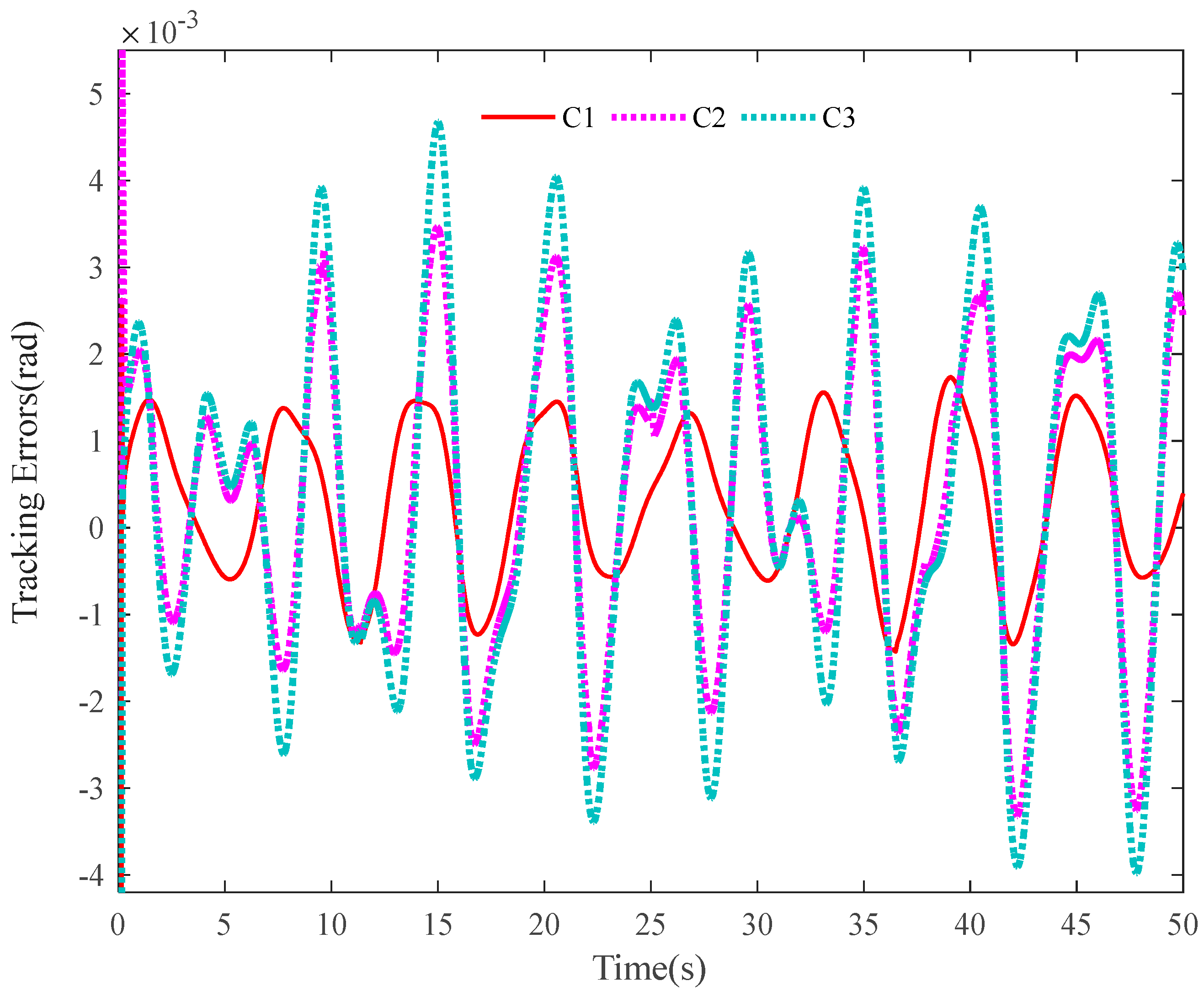
4.2. Comparative Results

(1)
C1: It is the proposed controller in Section 3. Its design parameters are picked in Table 2.
(2)
C2: It is same as C1 but without disturbance compensation. Notably, k3 = diag{350, 350}.
(3)
C3: It is the backstepping based feedback controller.
Table 2. The design parameters of C1.
The gains of the controllerk1 = diag{80, 500},
k2 = diag{200, 500},
k3 = diag{300, 300},
ke = diag{5, 5}
The bandwidths of the observersωo1 = diag{350, 350},
ωo2 = diag{500, 500}
The activation functions of the MLNN ψ 2 ( ) = tanh( ),
ψ 3 ( ) = tanh( ),
ψ d c ( ) =   1 e P a P b θ d c 1 , if   P a P b > 0         0 , otherwise
The gains of the MLNN adaptive lawsϒW2 = [1 × 10²I11, 1 × 10²I11]T,
ϒV2 = [1 × 10⁴I5, 1 × 10⁴I5]T,
ϒW3 = [8 × 101I14, 8 × 101I14]T,
ϒV3 = [1 × 10⁴I7, 1 × 10⁴I7]T,
ϒdc = [1 × 10³I14, 5 × 10²I14]T,
γW2 = [1 × 10⁻¹I11, 1 × 10⁻¹I11]T,
γV2 = [1 × 10⁻¹I5, 1 × 10⁻¹I5]T,
γW3 = [1 × 10⁻¹I14, 1 × 10⁻¹I14]T,
γV3 = [1 × 10⁻¹I7, 1 × 10⁻¹I7]T,
γdc = [1 × 10⁻¹I14, 1 × 10⁻¹I14]T
The gains of the filtersωc1 = diag{3 × 10³, 3 × 10³},
ωc2 = diag{3.2 × 10³, 3.2 × 10³}
Other parameterse0 = [1 × 10⁻¹, 1 × 10⁻¹]T,
u ¯ = [10, 10]T, u _ = [–10, –10]T
Notably, all controller parameters of C2 and C3 are chosen to be same as those of C1, except for those already mentioned.
The tracking errors of the three controllers for the two links can be found in Figure 2 and Figure 3. From them, it can be easily seen that the proposed C1 controller has the best tracking performance. By comparing the results of C1 and C2, C1 and C3, or C2 and C3, the ability to reject matched and mismatched disturbances of C1 can be proved. Furthermore, the state estimation performance of Link 1 and Link 2 with C1 can be found in Figure 4 and Figure 5, respectively. As shown, the high-accuracy estimation performance of the proposed observers can be verified. Meanwhile, from Figure 6, Figure 7, Figure 8 and Figure 9, bounded and regular disturbance and function estimation can further demonstrate the effectiveness of the designed observers. Additionally, from Figure 10, the control torques of Link 1 and Link 2 with C1 are both regular and meanwhile bounded.

5. Conclusions

This paper proposes a novel high-performance multilayer neuroadaptive algorithm for trajectory tracking control of n-DOF electro-hydraulic robotic manipulators. Notably, the developed controller can simultaneously compensate for smooth and non-smooth modeling uncertainties via multilayer neural networks. Meanwhile, matched and mismatched time-varying disturbances can be compensated by using the design technology of extended state observer. Moreover, the proposed algorithm can be suitable for the scene where the joint angular velocities are not measurable and can be free of the “explosion of complexity” generated by the conventional backstepping design method. Furthermore, the proposed controller has the advantages of anti-noise and anti-input-saturation, which puts it in front of the existing control algorithms.

Author Contributions

G.Y.: Conceptualization, Methodology, Software, Investigation, Writing-Original Draft, Writing-Review & Editing. Z.S.: Formal analysis. All authors have read and agreed to the published version of the manuscript.

Funding

This research received no external funding.

Data Availability Statement

The data are available from the corresponding author on reasonable request.

Conflicts of Interest

There are no conflicts of interest regarding the publication of this article.

Appendix A

Proof of Theorem 1.
When |εsat| ≥ ε0, we define the Lyapunov function candidate VL as
V L = 1 2 i = 1 3 z i T z i + i = 1 3 φ i T φ i + e sat T e sat + e o T P o e o + ε o T Q o ε o + j = 1 2 ς j T P c ς j + 1 2 t r W ˜ 2 T ϒ W 2 1 W ˜ 2 + t r V ˜ 2 T ϒ V 2 1 V ˜ 2 + t r W ˜ 3 T ϒ W 3 1 W ˜ 3 + t r V ˜ 3 T ϒ V 3 1 V ˜ 3 + t r W ˜ d c T ϒ d c 1 W ˜ d c
Differentiating (A1) along (16), (17), (24), (26), (29), (32), (35), (36) and (37), we can organize V ˙ L as
V ˙ L i = 1 3 κ z i z i 2 + i = 1 3 κ φ i φ i 2 + κ e s e sat 2 + κ e o e o 2 + κ ε o ε o 2 j = 1 2 κ ς j ς j 2 + j = 1 2 κ W ( j + 1 ) W ˜ j + 1 2 + j = 1 2 κ V ( j + 1 ) V ˜ j + 1 2 + κ W d c W ˜ d c 2 + Δ L
where κzi, κφi, κes, κeo, κεo, κςj, κW(j+1), κV(j+1), κWdc and ΔL are some unknown positive constants.
Based on (A2), we have
V ˙ L λ L V L + Δ L
where λL = 2min{κzi, κφi, κes, κeo/σmax(Po), κεo/σmax(Qo), κςj/σmax(Pc), κW2/σmax ( Υ W 2 1 ) , κV2/σmax ( Υ V 2 1 ) , κW3/σmax ( Υ W 3 1 ) , κV3/σmax ( Υ V 3 1 ) , κWdc/σmax ( Υ d c 1 ) }.
It can be inferred from (A1) and (A3) that z1, z2, z3, φ1, φ2, φ3, esat, eo,εo, ς1, ς2, W ~ 2 , V ~ 2 , W ~ 3 , V ~ 3 and W ~ d c belong to L when ΔL is bounded. According to Assumption 1, Assumption 3, (17), (18), (24), (26), (29), (32), (35) and (36), we can infer that all system states belong to L. Furthermore, from (34), the boundness of τ can be obtained. Consequently, all signals in the closed-loop hydraulic manipulator system can always stay bounded, which means that Theorem 1 can eventually be proved. □
When |εsat| < ε0, the Theorem 1 can also be proven according to the aforementioned procedures.

References

  1. Guo, Q.; Wang, Q.; Zuo, Z.; Zhang, Y.; Jiang, D.; Shi, Y. Parametric adaptive control of electro-hydraulic system driving two-DOF robotic arm. In Proceedings of the IEEE 56th Annual Conference on Decision and Control, Melbourne, VIC, Australia, 12–15 December 2017; pp. 3283–3288. [Google Scholar]
  2. Yang, G. State filtered disturbance rejection control. Nonlinear Dyn. 2024, 1–17. [Google Scholar] [CrossRef]
  3. Xia, Y.; Nie, Y.; Chen, Z.; Lyu, L.; Hu, P. Motion control of a hydraulic manipulator with adaptive nonlinear model compensation and comparative experiments. Machines 2022, 10, 214. [Google Scholar] [CrossRef]
  4. Yang, G.; Yao, J. Multilayer neurocontrol of high-order uncertain nonlinear systems with active disturbance rejection. Int. J. Robust Nonlinear Control 2024, 34, 2972–2987. [Google Scholar] [CrossRef]
  5. Chen, S.; Chen, Z.; Yao, B. Precision cascade force control of multi-DOF hydraulic leg exoskeleton. IEEE Access 2018, 6, 8574–8583. [Google Scholar] [CrossRef]
  6. Bu, F.; Yao, B. Nonlinear model based coordinated adaptive robust control of electro-hydraulic robotic manipulators: Methods and comparative studies. In Proceedings of the ASME International Mechanical Engineering Congress and Exposition, New York, NY, USA, 11–16 November 2001; pp. 651–659. [Google Scholar]
  7. Zhou, S.; Shen, C.; Xia, Y.; Chen, Z.; Zhu, S. Adaptive robust control design for underwater multi-DoF hydraulic manipulator. Ocean Eng. 2022, 248, 110822. [Google Scholar] [CrossRef]
  8. Petrović, G.R.; Mattila, J. Mathematical modelling and virtual decomposition control of heavy-duty parallel–serial hydraulic manipulators. Mech. Mach. Theory 2022, 170, 104680. [Google Scholar] [CrossRef]
  9. Koivumäki, J.; Mattila, J. Stability-guaranteed force-sensorless contact force/motion control of heavy-duty hydraulic manipulators. IEEE Trans. Rob. 2015, 31, 918–935. [Google Scholar] [CrossRef]
  10. Rigatos, G.; Zervos, N.; Abbaszadeh, M.; Pomares, J.; Wira, P. Non-linear optimal control for multi-DOF electro-hydraulic robotic manipulators. IET Cyber-Syst. Robot. 2020, 2, 96–106. [Google Scholar] [CrossRef]
  11. Yang, G.; Yao, J.; Dong, Z. Neuroadaptive learning algorithm for constrained nonlinear systems with disturbance rejection. Int. J. Robust Nonlinear Control 2022, 32, 6127–6147. [Google Scholar] [CrossRef]
  12. Dao, H.V.; Ahn, K.K. Extended sliding mode observer-based admittance control for hydraulic robots. IEEE Rob. Autom. Lett. 2022, 7, 3992–3999. [Google Scholar] [CrossRef]
  13. Shen, M.; Wang, X.; Park, J.H.; Yi, Y.; Che, W.W. Extended disturbance-observer-based data-driven control of networked nonlinear systems with event-triggered output. IEEE Trans. Syst. Man Cybern. Syst. 2023, 53, 3129–3140. [Google Scholar] [CrossRef]
  14. Zhang, X.; Shi, G. Dual extended state observer-based adaptive dynamic surface control for a hydraulic manipulator with actuator dynamics. Mech. Mach. Theory 2022, 169, 104647. [Google Scholar] [CrossRef]
  15. Dinh, T.X.; Thien, T.D.; Anh, T.H.V.; Ahn, K.K. Disturbance observer based finite time trajectory tracking control for a 3 DOF hydraulic manipulator including actuator dynamics. IEEE Access 2018, 6, 36798–36809. [Google Scholar] [CrossRef]
  16. Dao, H.V.; Tran, D.T.; Ahn, K.K. Active fault tolerant control system design for hydraulic manipulator with internal leakage faults based on disturbance observer and online adaptive identification. IEEE Access 2021, 9, 23850–23862. [Google Scholar] [CrossRef]
  17. Tran, D.T.; Truong, H.V.A.; Ahn, K.K. Adaptive backstepping sliding mode control based RBFNN for a hydraulic manipulator including actuator dynamics. Appl. Sci. 2019, 9, 1265. [Google Scholar] [CrossRef]
  18. Yang, G. Multilayer neuroadaptive constraint-handling control architecture for a family of nonlinear systems with uncertainty compensation. Inf. Sci. 2025, 690, 121517. [Google Scholar] [CrossRef]
  19. Selmic, R.R.; Lewis, F.L. Neural-network approximation of piecewise continuous functions: Application to friction compensation. IEEE Trans. Neural Netw. 2002, 13, 745–751. [Google Scholar] [CrossRef] [PubMed]
  20. Han, J. From PID to active disturbance rejection control. IEEE Trans. Ind. Electron. 2009, 56, 900–906. [Google Scholar] [CrossRef]
  21. He, W.; Dong, Y.; Sun, C. Adaptive neural impedance control of a robotic manipulator with input saturation. IEEE Trans. Syst. Man Cybern. Syst. 2016, 46, 334–344. [Google Scholar] [CrossRef]
  22. Gao, Z. Active disturbance rejection control: A paradigm shift in feedback control system design. In Proceedings of the 2006 American Control Conference, Minneapolis, MN, USA, 14–16 June 2006; pp. 2399–2405. [Google Scholar]
  23. Guo, B.Z.; Zhao, Z.L. On the convergence of an extended state observer for nonlinear systems with uncertainty. Syst. Control Lett. 2011, 60, 420–430. [Google Scholar] [CrossRef]
  24. Gao, Z. On the centrality of disturbance rejection in automatic control. ISA Trans. 2014, 53, 850–857. [Google Scholar] [CrossRef] [PubMed]
  25. Yang, G. Asymptotic tracking with novel integral robust schemes for mismatched uncertain nonlinear systems. Int. J. Robust Nonlinear Control 2023, 33, 1988–2002. [Google Scholar] [CrossRef]
  26. Farrell, J.A.; Polycarpou, M.; Sharma, M.; Dong, W. Command filtered backstepping. IEEE Trans. Autom. Control 2009, 54, 1391–1395. [Google Scholar] [CrossRef]
Figure 1. The structure diagram of a n-DOF serial hydraulic robotic manipulator.
Mathematics 13 00683 g001
Figure 2. Tracking errors of Link 1.
Mathematics 13 00683 g002
Figure 3. Tracking errors of Link 2.
Mathematics 13 00683 g003
Figure 4. State estimation performance of Link 1 with C1.
Mathematics 13 00683 g004
Figure 5. State estimation performance of Link 2 with C1.
Mathematics 13 00683 g005
Figure 6. Disturbance estimation of Link 1 with C1.
Mathematics 13 00683 g006
Figure 7. Disturbance estimation of Link 2 with C1.
Mathematics 13 00683 g007
Figure 8. Function estimation of Link 1 with C1.
Mathematics 13 00683 g008
Figure 9. Function estimation of Link 2 with C1.
Mathematics 13 00683 g009
Figure 10. Control torques.
Mathematics 13 00683 g010
Table 1. System parameters.
ParameterValue (Unit)ParameterValue (Unit)
Jm15.2 (kg)L100.2 (m)
Jm26.2 (kg)L110.2 (m)
JI12.25 (kg•m2)L120.2 (m)
JI21.25 (kg•m2)Ps50 (bar)
JL15.2 (kg)Pr0 (bar)
Sc10.2 (m)βef1.26 × 109 (Pa)
Sc20.15 (m)Aa111 × 10−3 (m2)
S10.5 (m)Ab115 × 10−4 (m2)
S20.2 (m)Aa221.22 × 10−4 (m3/rad)
Ctl11, Ctl222.8 × 10−12 (m3/s/Pa)Ab221.22 × 10−4 (m3/rad)
Cd11ωd11Kg11 2 ρ o 3.2 × 10⁻⁸ (m3/s/V/ P a )Cd22ωd22Kg22 2 ρ o 2.2 × 10⁻⁸ (m3/s/V/ P a )
Disclaimer/Publisher’s Note: The statements, opinions and data contained in all publications are solely those of the individual author(s) and contributor(s) and not of MDPI and/or the editor(s). MDPI and/or the editor(s) disclaim responsibility for any injury to people or property resulting from any ideas, methods, instructions or products referred to in the content.

