Approximate Description of Indefinable Granules Based on Classical and Three-Way Concept Lattices

Abstract

Granule description is a fundamental problem in granular computing. However, how to describe indefinable granules is still an open, interesting, and important problem. The main objective of this paper is to give a preliminary solution to this problem. Before proceeding, the framework of approximate description is introduced. That is, any indefinable granule is characterized by an ordered pair of formulas, which form an interval set, where the first formula is the $\beta$-prior approximate optimal description and the second formula is the $\alpha$-prior approximate optimal description. More concretely, given an indefinable granule, by exploring the description of its lower approximate granule, its $\beta$-prior approximate optimal description is obtained. Likewise, by consulting the description of its upper approximate granule, its $\alpha$-prior approximate optimal description can also be derived. Following this idea, the descriptions of indefinable granules are investigated. Firstly, ∧-approximate descriptions of indefinable granules are investigated based on the classical concept lattice, and $(\wedge ,\vee )$-approximate descriptions of indefinable granules are given via object pictorial diagrams. And then, it is revealed from some examples that the classical concept lattice is no longer effective and negative attributes must be taken into consideration. Therefore, a three-way concept lattice is adopted instead of the classical concept lattice to study $(\wedge ,\neg )$-approximate descriptions and $(\wedge ,\vee ,\neg )$-approximate descriptions of indefinable granules. Finally, some discussions are presented to show the differences and similarities between our study and existing ones.

1. Introduction

Granular computing (GrC) is a discipline that specializes in the theoretical, methodological, technical, and tool approaches to problem-solving and information processing of information granules and their structures in datasets [1,2,3]. Any methodologies, theories and tools that treat complex information entities in different levels of granules fall into the scope of granular computing [1,2,3,4,5]. The concept of granular computing has been widely used in many research fields, such as cognitive science and cognitive informatics [6].

Although different systems may have different external differences, information granules can be identified based on their essential similarities, which may include functional or physical adjacency, coherency, and the like [7,8]. Once information granules are obtained, they can be combined and used to construct more complicated hierarchical structures. Moreover, by shifting from one level to another level, we can obtain important clues to solve many complicated problems [9,10].

No matter what we want to do with the information granules, the first step is to characterize the research object. Furthermore, if we want to communicate with other granules and intelligent machines, we still have to find a concise way to explicitly depict these granules. Then, descriptions of granules deserve our great concern [11]. Studies of granule description can not only help achieve a profound understanding of the discussed question, but also shed light on some unsolved psychological problems. Generally speaking, any research which tries to find a good description of the subset of the problem space falls within the scope of granule description. In a narrow sense, granule description is aimed at finding a logical formula that best describes a given granule.

There are two crucial issues in granule description. The first step is to select a scheme that best fits the objective of the problem under consideration. For example, if we want to investigate the features shared by different granules, we have to choose common attribute analysis. At this time, we will derive a series of formal concepts [12]. However, if we want to know which features are possessed by a granule but are not possessed by other granules, we must resort to necessary attribute analysis. At this time, we will derive a collection of object-oriented concepts [13]. Therefore, it is not surprising that a granule is definable via common attribute analysis but it may become indefinable via necessary attribute analysis, and vice versa. The other issue is the selection of basic definable granules which can be used to approximate more complicated indefinable granules. For example, in knowledge representation, basic granules are used as the building blocks by which more complex granules can be characterized via logic connections [11,14,15,16]. In cognitive learning processes, basic granules, known as granular concepts, are always the starting point from which complicated concepts can be derived by incorporating new information [17].

Two strategies are frequently used in the descriptions of granules and related studies. One is the set approximation from rough set theory (RST), presented by Pawlak [18]; the other is the extension-intension view highlighted in formal concept analysis (FCA) [19]. Some scholars have explained that RST and FCA are essentially related to each other and are two effective methods of granular computing [20,21,22,23]. Essentially, these two theories have the same opinion with respect to granule description. That is, they first select a scheme to obtain a collection of basic granules, and then adopt approximations to characterize other granules. However, there are differences between them. Compared to RST, FCA establishes a partial order between granules and gives each granule a unique label to explicitly show the corresponding intension. Generally speaking, RST is good at describing a target set based on similar objects, while FCA is skilled at providing the description of a granule by using a set of attributes. So, which one is better greatly depends on our requirements.

After several years of rapid development, RST has become a useful tool for uncertain data management [24]. In the study of granule description in RST, indefinable granules are actually the ones that contain uncertain parts. In other words, there exist granules that cannot be described by basic knowledge. Then, an alternative approach is provided to solve this problem by using a pair of lower and upper approximations. Furthermore, the precision of this model is measured by the fraction of the lower approximation to the upper approximation. Motivated by the requirements of multi-source information fusion, multigranulation rough sets have become a hot research field in RST [25]. After all kinds of generalizations, many new types of multigranulation rough sets were presented to fit different types of information systems, such as incomplete, neighborhood, covering, and fuzzy information systems [26,27].

RST can be integrated with FCA to improve the ability of granule representation. For example, by combining concept approximation of RST with the concept-building strategies of FCA, AFS-concept [14], property-oriented concepts [21], and the object-oriented concept lattice [13] have been presented to meet different requirements. Moreover, basic terms of granular computing can be directly applied in these generalized concept lattices to define important notions, such as granular concept and granular rule [28]. The basic ideas of granular computing can also be combined with optimization algorithms to make decisions [29]. Moreover, some studies have shown that negative attributes are of equal importance as positive ones in characterizing a target granule [30]. In these studies, only positive attributes were used to describe a given granule while negative ones were ignored.

Three-way concept analysis (3WCA), a combination of three-way decisions [31,32] and FCA, proposed by Qi et al. [33], has become a hot topic [17,34,35,36,37]. In fact, 3WCA not only develops FCA but also provides a way to understand problems from both positive and negative perspectives. Three-way concept lattices can be built based on formal concept lattices [38], and they can enable us to describe granules from a more broad and profound perspective.

Until now, granule description has involved a few preliminary explorations. By combining the merits of RST and FCA, Yao [16] interpreted the notions of RS-definable concepts and the Boolean algebra of RS-definable concepts. An interesting conclusion was obtained in Yao [16]. That is, RS-definable concepts can serve as the basic knowledge to approximate RS-indefinable concepts. Necessary attribute analysis was proposed, and RS-definable concepts are identical to object-oriented concepts as reported in our previous work [39]. Thus, describing indefinable granules becomes a more interesting and appealing problem.

To this end, this paper focus on the descriptions of indefinable granules. The main contribution of this paper is as follows: Given an indefinable granule, we first find two definable granules to approximate this indefinable granule. That is, one granule serves as its lower approximate granule and the other serves as its upper approximate granule. Then, we use the description of its lower approximate granule as its $\beta$-prior approximate optimal description and use the description of its upper approximate granule as its $\alpha$-prior approximate optimal description. Finally, we characterize this indefinable granule by an ordered pair of formulas, which actually form an interval set, where the first formula is the $\beta$-prior approximate optimal description and the second formula is the $\alpha$-prior approximate optimal description.

Following this idea, the description of indefinable granules is investigated. The remainder of the paper is organized as follows: In Section 2, we review some basic notions, such as formal concept analysis, three-way concept analysis, and Pawlak’s rough set. In Section 3, we discuss the fundamentals of approximate descriptions. In Section 4, we propose approximate description methods of granules-based FCA. Concretely, we first investigate ∧-approximate descriptions based on a concept lattice. Next, we continue studying $(\wedge ,\vee )$-approximate descriptions of granules based on an object pictorial diagram. In Section 5, we present $(\wedge ,\neg )$-approximate descriptions and $(\wedge ,\vee ,\neg )$-approximate descriptions of granules based on 3WCA, respectively. In Section 6, we present a case study and experimental analysis. Finally, some discussions are given in Section 7.

2. Preliminaries

In this section, we review some basic notions to make our paper self-contained.

2.1. Basic Notions in FCA

Let G be a domain. Then, all possible granules form a power set of G, denoted as $2^G$. However, at best, only a small proportion of the granules can be studied in a certain theory. This is also true for FCA. As one of the rapidly developing research areas of granular computing, FCA concerns the granules that fulfill some rigid constraints.

As is well known, FCA starts with a formal context, which is usually represented as a triple $K=(G,M,I)$, where G is a set of objects, M is a set of attributes, and $I\subseteq G\times M$ specifies the relation between G and M.

A formal concept is a pair $(X,A)$ [12], where $X\subseteq G$, $A\subseteq M$, $X^{\ast }=\{a\in M|\forall x\in X,xIa\}=A$, and $A^{\ast }=\{x\in G|\forall a\in A,xIa\}=X$. Moreover, X and A are called the extent and the intent of the concept $(X,A)$, respectively. In addition, we use $\mathrm{ext}(X,A)$ and $\mathrm{int}(X,A)$ to denote the extent and the intent of the concept $(X,A)$, respectively.

Let $(X_1,A_1)$ and $(X_2,A_2)$ be two formal concepts. Then, the partial order ${\le }_F$ is defined  by:

$$(X_1,A_1){\le }_F(X_2,A_2)\iff X_1\subseteq X_2\iff A_1\supseteq A_2.$$

Furthermore, if there does not exist another concept $(X_3,A_3)$ such that $(X_1,A_1)\le F(X_3,A_3)\le F(X_2,A_2)$, we call $(X_1,A_1)$ a lower neighbor of $(X_2,A_2)$, or $(X_2,A_2)$ an upper neighbor of $(X_1,A_1)$, denoted by $(X_1,A_1){\prec }_F(X_2,A_2)$.

Then, the concept lattice of K, denoted as $L\left(K\right)$, is constituted by all the formal concepts together with the partial order ${\le }_F$.

2.2. Basic Notions in 3WCA

Let M be an attribute set and $2^M\times 2^M$ be the Cartesian product of $2^M$ and $2^M$. Then, we introduce a partial order ≤ in $2^M\times 2^M$:

$(A_1,A_2)\le (B_1,B_2)\iff A_1\subseteq B_1,A_2\subseteq B_2.$

Moreover, we define $(A_1,A_2)=(B_1,B_2)\iff A_1=B_1,A_2=B_2$. The intersection ∩ and the union ∪ in $2^M\times 2^M$ are, respectively, defined as:

$(A_1,A_2)\cap (B_1,B_2)=(A_1\cap B_1,A_2\cap B_2),$

$(A_1,A_2)\cup (B_1,B_2)=(A_1\cup B_1,A_2\cup B_2).$

For a formal context $K=(G,M,I)$, let $X^{\stackrel{-}{\ast }}=\{a\in M|\forall x\in X,x{I}^{c}a\}$ and $B^{\stackrel{-}{\ast }}=\{x\in G|\forall a\in B,x{I}^{c}a\}$, where $I^c=G\times M-I$. Then, a three-way formal concept is a pair $(X,(A,B\left)\right)$ [33], where $X^p=(X^{\ast },X^{\stackrel{-}{\ast }})=(A,B)$ and ${(A,B)}^q=A^{\ast }\cap B^{\stackrel{-}{\ast }}=X$. In this case, X and $(A,B)$ are called the extent and intent of $(X,(A,B\left)\right)$, respectively. In addition, we use $\mathrm{ext}(X,(A,B\left)\right)$ and $\mathrm{int}(X,(A,B\left)\right)$ to denote the extent and the intent of the three-way concept $(X,(A,B\left)\right)$, respectively.

Let $(X_1,(A_1,B_1))$ and $(X_2,(A_2,B_2))$ be two three-way formal concepts. Then, the partial order ${\le }_T$ is defined by:

$$(X_1,(A_1,B_1)){\le }_T(X_2,(A_2,B_2))\iff X_1\subseteq X_2\iff (A_1,B_1)\ge (A_2,B_2).$$

Furthermore, if there does not exist another three-way formal concept $(X_3,(A_3,B_3))$ such that $(X_1,(A_1,B_1)){\le }_T(X_3,(A_3,B_3)){\le }_T(X_2,(A_2,B_2))$, we call $(X_1,(A_1,B_1))$ a lower neighbor of $(X_2,(A_2,B_2))$, or $(X_2,(A_2,B_2))$ an upper neighbor of $(X_1,(A_1,B_1))$, denoted by $(X_1,(A_1,B_1)){\prec }_T(X_2,(A_2,B_2))$.

Similarly, the three-way concept lattice of K, denoted as $TL\left(K\right)$, is constituted by all the three-way formal concepts together with the partial order ${\le }_T$.

2.3. Basic Notions in RST

Let $S=(U,AT,R)$ be an information system, $X\subseteq U$ be a target set, and $A\subseteq AT$, where the finite nonempty set U is the universe, the finite nonempty set $AT$ is the attributes, and R specifies the relations between the universe and the attributes.

Then, we can describe any target set X in two steps:

(i) Based on the following equivalence relation

$$IND\left(A\right)=\left\{\right(x,y)\in U\times U\mid \forall a\in A,R(x,a)=R(y,a\left)\right\},$$

we partition the universe U into equivalence classes ${\left[x\right]}_A=\{y\in U\mid (x,y)\in IND\left(A\right)\}$.

(ii) We approximate the target set X by a pair $[\underline{A}\left(X\right),\overline{A}\left(X\right)]$, where

$$\underline{A}\left(X\right)=\{x\in U\mid {\left[x\right]}_A\subseteq X\}\mathrm{and}\overline{A}\left(X\right)=\{x\in U\mid {\left[x\right]}_A\cap X\ne Ø\}.$$

Furthermore, the accuracy of this approximate description is $\rho \left(X\right)={\displaystyle \frac{|\underline{A}\left(X\right)|}{|\overline{A}\left(X\right)|}},$ where $|·|$ denotes the cardinality of a set.

According to Pawlak’s rough set [18], definable granules have the following properties:

(i) Both ∅ and U are definable granules;

(ii) If X and Y are definable granules, then $X\cap Y$ is a definable granule;

(iii) If X and Y are definable granules, then $X\cup Y$ is a definable granule;

(iv) If X is a definable granule, then $U-X$ is also a definable granule.

In this paper, the ideas of upper and lower approximations will be incorporated into the descriptions of indefinable granules. Furthermore, logic connectives ∧, ∨, and ¬ will be used to establish description formulas, and they correspond to ∩, ∪, and − in the set-theoretic formulation method of RST.

3. Approximate Description Based on Logic Language

In this section, we present the fundamentals of granule description and investigate the descriptive abilities of description languages.

3.1. Fundamentals of Granule Description

Logic language, originating from the decision logic language, is a very important language used in knowledge discovery [40].

In this paper, atomic formulas are denoted by lowercase letters, such as a, b, and c. When a set of atomic formulas is considered, more complicated formulas can be obtained by recursively using logic connectives, such as ¬, ∧, ∨, →, and ↔.

Moreover, we give a language a name based on the logic connectives we use. For example, if only logic connectives ∧ and ¬ are used in a language, we call this language a $(\wedge ,\neg )$-language.

Furthermore, it should be pointed out that the discussion on the descriptions of granules will be confined to a certain predefined language.

Let G be a nonempty set of individuals and K be a knowledge base with respect to G. If an individual $x\in G$ satisfies a formula $\phi \in K$, then we denote this case as $x\vDash \phi$.

Definition 1 

([41]). The meaning of a formula φ is the set of individuals which satisfy the formula φ, i.e.,

$$m\left(\phi \right)=\{x\mid x\in G,x\vDash \phi \}.$$

According to Definition 1, it is easy to obtain the following Proposition 1.

Proposition 1 

([41]). Let φ and ψ be two formulas. Then, the following properties hold:

(i) $m(\neg \phi )=\neg m\left(\phi \right)$;

(ii) $m(\phi \wedge \psi )=m\left(\phi \right)\cap m\left(\psi \right)$;

(iii) $m(\phi \vee \psi )=m\left(\phi \right)\cup m\left(\psi \right)-m\left(\phi \right)\cap m\left(\psi \right)$;

(iv) $m(\phi \to \psi )=\neg m\left(\phi \right)\cup m\left(\psi \right)$;

(v) $m(\phi \equiv \psi )=\left(m\right(\phi )\cap m(\psi \left)\right)\cup (\neg m(\phi )\cap \neg m(\psi \left)\right)$.

Definition 2 

([39]). Let X be a granule and φ be a formula. The recall and precision indices of φ with respect to X are defined by:

$$\alpha (\phi ,X)={\displaystyle \frac{\left|m\right(\phi )\cap X|}{\left|X\right|}}and\beta (\phi ,X)={\displaystyle \frac{\left|m\right(\phi )\cap X|}{\left|m\right(\phi \left)\right|}}.$$

Note that if there is no confusion, we use $\alpha \left(\phi \right)$ and $\beta \left(\phi \right)$ instead of $\alpha (\phi ,X)$ and $\beta (\phi ,X)$ for the sake of convenience.

Definition 3. 

Let X be a granule, φ be a formula, and $x\in m\left(\phi \right)$. If $\beta \left(\phi \right)=1$, we say that x necessarily belongs to X, denoted by $x{\in }_{\ast }X$; if $0<\beta \left(\phi \right)<1$, we say that x possibly belongs to X, denoted by $x{\in }^{\ast }X$.

Definition 4. 

Let X be a granule and Φ be the set of all formulas of a language. If both $\alpha \left(\phi \right)$ and $\beta \left(\phi \right)$ have the biggest values among all the formulas in Φ, then we call φ the optimal description of the granule X.

For a given granule, there may not be a formula that has the biggest values $\alpha$ and $\beta$ simultaneously. So, Definition 4 is only theoretically sound. Thus, we have to find an approximate optimal description in a feasible manner. The following definition actually gives two kinds of approximate optimal descriptions, which take recall and precision into consideration in order.

Definition 5. 

Let X be a granule and Φ be the set of all formulas of a language. If $\alpha \left(\phi \right)=1$ and $\beta \left(\phi \right)$ has the biggest value among all the formulas in Φ, then we call φ the α-prior approximate optimal description of X, and denote it as $d^{\alpha \ast }\left(X\right)$. Correspondingly, if $\beta \left(\phi \right)=1$ and $\alpha \left(\phi \right)$ has the biggest value among all the formulas in Φ, then we call φ the β-prior approximate optimal description of X, and denote it as $d^{\beta \ast }\left(X\right)$.

By using Definition 3, we have the following propositions:

(i) if $x\in m\left(d^{\beta \ast }\left(X\right)\right)$, then $x{\in }_{\ast }X$;

(ii) if $x\in m\left(d^{\alpha \ast }\left(X\right)\right)$, then $x{\in }^{\ast }X$.

Proposition 2. 

Let X be a granule. Then, $m\left(d^{\beta \ast }\left(X\right)\right)\subseteq X\subseteq m\left(d^{\alpha \ast }\left(X\right)\right)$.

Theorem 1. 

Let X be a granule and Φ be the set of all formulas of a language. The α-prior approximate optimal description of X is:

$$d^{\alpha \ast }\left(X\right)=\underset{{\phi }_i\in \Psi }{\bigwedge }{\phi }_i,$$

where $\Psi =\{\phi \mid \phi \in \Phi ,\alpha (\phi )=1\}$.

Theorem 2. 

Let X be a granule and Φ be the set of all formulas of a language. The β-prior approximate optimal description of X is:

$$d^{\beta \ast }\left(X\right)=\underset{{\phi }_i\in \Psi }{\bigvee }{\phi }_i,$$

where $\Psi =\{\phi \mid \phi \in \Phi ,\beta (\phi )=1\}$.

Definition 6. 

Let X be a granule. We call $d^{\ast }\left(X\right)=[d^{\beta \ast }\left(X\right),d^{\alpha \ast }\left(X\right)]$ the approximate description of X. And the approximate description accuracy is defined by:

$$Acc\left(d^{\ast }\left(X\right)\right)={\displaystyle \frac{\left|m\right(d^{\beta \ast }\left(X\right)\left)\right|}{\left|m\right(d^{\alpha \ast }\left(X\right)\left)\right|}}.$$

Definition 7 

([41]). Let $2^U$ be the power set of U. Given a pair of sets $(X_1,X_2)$ with $X_1\subseteq X_2\subseteq U$,

$$[X_1,X_2]=\{X\in 2^U\mid X_1\subseteq X\subseteq X_2\}$$

is called a closed interval set.

Let X be a granule with its approximate description $d^{\ast }\left(X\right)$. Based on Proposition 2, it is easy to see that $m\left(d^{\ast }\left(X\right)\right)=[m\left(d^{\beta \ast }\left(X\right)\right),m\left(d^{\alpha \ast }\left(X\right)\right)]$ forms a closed interval set.

Definition 8. 

Let X be a granule with its approximate description $d^{\ast }\left(X\right)$. If $Acc\left(d^{\ast }\left(X\right)\right)=1$, we say that the granule X is definable; otherwise, we say that the granule X is indefinable.

Note that if X is definable, we use the denotation $d\left(X\right)$ instead of $d^{\ast }\left(X\right)$.

Proposition 3. 

Let X be a granule. The following properties are equivalent to each other:

(i) $Acc\left(d^{\ast }\left(X\right)\right)=1$;

(ii) $m\left(d^{\beta \ast }\left(X\right)\right)=m\left(d^{\alpha \ast }\left(X\right)\right)$;

(iii) There exists a formula φ such that $m\left(\phi \right)=X$;

(iv) There exists a formula φ such that $\alpha \left(\phi \right)=1$ and $\beta \left(\phi \right)=1$.

Proposition 4. 

Let X, $X_1$ and $X_2$ be granules. The following properties hold:

(i) $m(\neg d^{\ast }\left(X\right))=\setminus m\left(d^{\ast }\left(X\right)\right)$;

(ii) $m(d^{\ast }\left(X_1\right)\wedge d^{\ast }\left(X_2\right))=m\left(d^{\ast }\left(X_1\right)\right)\sqcap m\left(d^{\ast }\left(X_2\right)\right)$;

(iii) $m(d^{\ast }\left(X_1\right)\vee d^{\ast }\left(X_2\right))=m\left(d^{\ast }\left(X_1\right)\right)\bigsqcup m\left(d^{\ast }\left(X_2\right)\right)$;

(iv) $m(d^{\ast }\left(X_1\right)\to d^{\ast }\left(X_2\right))=\setminus m\left(d^{\ast }\left(X_1\right)\right)\bigsqcup m\left(d^{\ast }\left(X_2\right)\right)$;

(v) $m(d^{\ast }\left(X_1\right)\equiv d^{\ast }\left(X_2\right))=(\setminus m\left(d^{\ast }\left(X_1\right)\right)\bigsqcup m\left(d^{\ast }\left(X_2\right)\right))\sqcap (m\left(d^{\ast }\left(X_1\right)\right)\bigsqcup \setminus m\left(d^{\ast }\left(X_2\right)\right))$, where ∖, ⊓ and ⊔ are the interval-set complement, intersection, and union given in [42]. That is, for two interval sets $[X_1,X_2]$ and $[Y_1,Y_2]$,

$$\setminus [X_1,X_2]=[-X_2,-X_1],$$

$$[X_1,X_2]\sqcap [Y_1,Y_2]=[X_1\cap Y_1,X_2\cap Y_2],$$

$$[X_1,X_2]\bigsqcup [Y_1,Y_2]=[X_1\cup Y_1,X_2\cup Y_2].$$

Definition 9. 

Let X be an indefinable granule. $X_l$ is called a lower approximate granule of X if $X_l$ is definable and there does not exist another definable granule $Y_l$ such that $X_l\subset Y_l\subset X$. Correspondingly, $X_u$ is called an upper approximate granule of X if $X_u$ is definable and there does not exist another definable granule $Y_u$ such that $X_u\supset Y_u\supset X$.

Proposition 5. 

Let X be an indefinable granule, $X_l$ be its lower approximate granule and $X_u$ be its upper approximate granule. Then, $d\left(X_l\right)$ is its β-prior approximate optimal description and $d\left(X_u\right)$ is its α-prior approximate optimal description.

Definition 10. 

Let X be a granule. The recall and precision indices of the approximate optimal description of X are defined as:

$$\alpha \left(d^{\ast }\left(X\right)\right)=\alpha \left(d^{\beta \ast }\left(X\right)\right)and\beta \left(d^{\ast }\left(X\right)\right)=\beta \left(d^{\alpha \ast }\left(X\right)\right).$$

Proposition 6. 

Let X, $X_1$ and $X_2$ be granules. Then, the following properties hold:

(i) $\alpha \left(d^{\ast }\left(X\right)\right)=1-\alpha \left(d^{\ast }(\neg d^{\ast }\left(X\right))\right)$;

(ii) $\alpha (d^{\ast }\left(X_1\right)\wedge d^{\ast }\left(X_2\right))\le min\left\{\alpha \right(d^{\ast }\left(X_1\right),\alpha \left(d^{\ast }\left(X_2\right)\right\}$;

(iii) $\alpha (d^{\ast }\left(X_1\right)\vee d^{\ast }\left(X_2\right))\ge max\left\{\alpha \right(d^{\ast }\left(X_1\right),\alpha \left(d^{\ast }\left(X_2\right)\right\}$;

(iv) $\alpha (d^{\ast }\left(X_1\right)\vee d^{\ast }\left(X_2\right))=\alpha \left(d^{\ast }\left(X_1\right)\right)+\alpha \left(d^{\ast }\left(X_2\right)\right)-\alpha (d^{\ast }\left(X_1\right)\wedge d^{\ast }\left(X_2\right))$.

It is necessary to point out that the following properties do not hold:

(i) $\beta \left(d^{\ast }\left(X\right)\right)=1-\beta \left(d^{\ast }(\neg d^{\ast }\left(X\right))\right)$;

(ii) $\beta (d^{\ast }\left(X_1\right)\wedge d^{\ast }\left(X_2\right))\le min\left\{\beta \right(d^{\ast }\left(X_1\right),\beta \left(d^{\ast }\left(X_2\right)\right\}$;

(iii) $\beta (d^{\ast }\left(X_1\right)\vee d^{\ast }\left(X_2\right))\ge max\left\{\beta \right(d^{\ast }\left(X_1\right),\beta \left(d^{\ast }\left(X_2\right)\right\}$;

(iv) $\beta (d^{\ast }\left(X_1\right)\vee d^{\ast }\left(X_2\right))=\beta \left(d^{\ast }\left(X_1\right)\right)+\beta \left(d^{\ast }\left(X_2\right)\right)-\beta (d^{\ast }\left(X_1\right)\wedge d^{\ast }\left(X_2\right))$.

Actually, Definition 9 and Proposition 5 manifest our main idea about the approximate description of indefinable granules. That is, given an indefinable granule, we first find two definable granules to serve as its lower and upper approximate granules. And then, we use the descriptions of these two approximate granules to construct the approximate description of this indefinable granule.

3.2. Descriptive Abilities of Description Languages

The fact that some concepts seem to be difficult, complicated, and incoherent, while others are psychologically easy and simple to be understood has widely been accepted by cognitive scientists. Some experiments have demonstrated that two factors strongly affect the difficulty of describing a concept. One factor is the length of the descriptive formulas for the concepts, and the other factor is the logic connectives used in the descriptive formula. Generally speaking, the shorter the descriptive formula is, the less difficult the concept seems to be. Moreover, disjunctive (‘Or’) concepts are hard to learn compared with conjunctive (‘And’) concepts. These finding may partly explain the phenomenon why the descriptive logics used in existing studies mainly rely on conjunctive formulas, such as the ones in the traditional FCA and rough set theory. Only a few studies have used disjunctive formulas, such as those in monotone concepts [14,43], multigranulation rough sets [44], and negative association rules [30].

Note that indefinable granules are defined in Definition 8. In fact, the discussions about whether a granule is definable only make sense under a predefined logic language. On most occasions, if we resort to a more powerful logic language, some indefinable granules will become definable.

Definition 11 

([39]). Let X be a granule. If only the logic connective ∧ is enough in the description of X, we say that it is a ∧-definable granule; if the logic connectives ∧ and ¬ are enough in the description of X, we say that it is a $(\wedge ,\neg )$-definable granule; if the logic connectives ∧ and ∨ are enough in the description of X, we say that it is a $(\wedge ,\vee )$-definable granule.

It is obvious that all the ∧-definable granules are both $(\wedge ,\neg )$-definable and $(\wedge ,\vee )$-definable.

Definition 12. 

Let X be a granule. If the logic connectives ∧, ∨, and ¬ are enough in the description of X, we say that it is a $(\wedge ,\vee ,\neg )$-definable granule. Moreover, if a granule is $(\wedge ,\vee ,\neg )$-indefinable, we say it is absolutely indefinable.

Remark 1. 

Whether a granule is definable or not depends on the description logic language we use and the perspective from which we look at the problem.

Example 1. 

Consider the formal context $K=(G,M,I)$ shown in

Table 1. A formal context $K=(G,M,I)$.

	a	b	c
1		∗
2	∗	∗
3		∗	∗

, where $G=\{1,2,3\}$ and $M=\{a,b,c\}$.

It is easy to observe that $\left\{1\right\}$ is a ∧-indefinable granule. Moreover, we can show that both $\left\{2\right\}$ and $\left\{3\right\}$ are ∧-definable granules. However, if we take the logic connective ¬ into consideration, then the granule $\left\{1\right\}$ will also become $(\wedge ,\neg )$-definable, and has a description $b\wedge \neg c$.

Take a different perspective and consider the complement formal context shown in

Table 2. The complement formal context of the one shown in Table 1.

	a	b	c
1	∗		∗
2			∗
3	∗

(see Table 1). In this formal context, $\left\{1\right\}$ turns out to be a ∧-definable granule. Meanwhile, both $\left\{2\right\}$ and $\left\{3\right\}$ turn out to be ∧-indefinable granules. But if the connective ¬ is adopted in the descriptive language, both $\left\{2\right\}$ and $\left\{3\right\}$ are $(\wedge ,\neg )$-definable granules.

It is well known that ∧-definable granules play an important role in FCA and concept learning, while $(\wedge ,\neg )$-definable granules have an intimate relationship with 3WCA and three-way decisions [37,45,46]. So, we will investigate ∧, $(\wedge ,\vee )$-indefinable granules and $(\wedge ,\neg )$, $(\wedge ,\vee ,\neg )$-indefinable granules based on FCA and 3WCA in the subsequent discussions.

In what follows, we discuss the relations between $(\wedge ,\neg )$-indefinable granules and $(\wedge ,\vee )$-definable granules, and those between $(\wedge ,\neg )$-definable granules and $(\wedge ,\vee )$-indefinable granules.

Remark 2. 

Some $(\wedge ,\neg )$-indefinable granules can be $(\wedge ,\vee )$-definable.

Example 2. 

Consider the formal context $K=(G,M,I)$ shown in

Table 3. A formal context $K=(G,M,I)$.

	a	b	c	d	e	f	g
1	∗					∗
2	∗					∗	∗
3	∗	∗					∗
4	∗		∗		∗
5	∗	∗	∗		∗
6		∗	∗	∗
7		∗	∗		∗

, where $G=\{1,2,3,4,5,6,7\}$ and $M=\{a,b,c,d,e,f,g\}$.

Note that we cannot find a formula containing the connectives ∧ and ¬ only to crisply describe $\{2,3,5\}$. So, $\{2,3,5\}$ is $(\wedge ,\neg )$-indefinable. On the other hand, since $m\left(\right(a\wedge b\wedge c)\vee g)=\{2,3,5\}$, we conclude that $\{2,3,5\}$ is $(\wedge ,\vee )$-definable.

Remark 3. 

Some $(\wedge ,\vee )$-indefinable granules can be $(\wedge ,\neg )$-definable.

Example 3. 

Continued with Example 2. Note that we cannot find a formula containing the connectives ∧ and ∨ only to describe $\{1,2,4\}$. So, $\{1,2,4\}$ is $(\wedge ,\vee )$-indefinable. On the other hand, since $m(a\wedge \neg b)=\{1,2,4\}$, we conclude that $\{1,2,4\}$ is $(\wedge ,\neg )$-definable.

Furthermore, it is obvious that all the $(\wedge ,\vee )$ and $(\wedge ,\neg )$-definable granules are also $(\wedge ,\vee ,\neg )$-definable granules. To sum up, the descriptive abilities of ∧, $(\wedge ,\neg )$, $(\wedge ,\vee )$ and $(\wedge ,\vee ,\neg )$-languages can be shown by Figure 1 in which the arrows from top to bottom represent stronger descriptive abilities.

It should be pointed out that the more powerful the language we use, the higher the description accuracy we will obtain and the more complicated the formula that should be used. Then, it is natural that we will usually make a tradeoff between the accuracy and the description complexity to cater to different applications. And this may be a satisfying explanation for the necessity of discussing approximate descriptions by using different logic languages.

4. Approximate Description Methods for Indefinable Granules Based on FCA

In this section, we will give some strategies on the approximate descriptions of indefinable granules based on FCA.

4.1. ∧-Approximate Descriptions of Indefinable Granules Based on the Concept Lattice

In this subsection, we explore the ∧-approximate descriptions of indefinable granules based on the concept lattice. Let $K=(G,M,I)$ be a formal context and $X\subseteq G$. If X is an extent of a formal concept of K, then we call X a basic granule.

Lemma 1. 

Let $K=(G,M,I)$ be a formal context and $X\subseteq G$ be a granule. If there exists a concept $(X,A)$ of $L\left(K\right)$, then X is ∧-definable.

Proof. 

Since there exists a concept with an extent equal to X, it is trivial to show that $m\left(\phi \right)=X$, where $\phi ={\displaystyle \underset{a\in A}{\bigwedge }}a$. Hence, X is ∧-definable.    □

Definition 13. 

Let $K=(G,M,I)$ be a formal context and $X\subseteq G$ be a granule. If there exist two concepts $(X_1,A_1)$ and $(X_2,A_2)$ such that $X_1\subseteq X\subseteq X_2$, we say that X is approximately ∧-definable.

Theorem 3. 

All granules are approximately ∧-definable.

Proof. 

Let $K=(G,M,I)$ be a formal context and $X\subseteq G$ be a granule. On the one hand, if there exists a concept of $L\left(K\right)$ with its extent equal to X, then X is ∧-definable based on Lemma 1. On the other hand, if there does not exist a concept with its extent equal to X, there must be two concepts $(G,G^{\ast })$ and $(M^{\ast },M)$ with their extents $M^{\ast }\subseteq X\subseteq G$. As the granules G and $M^{\ast }$ are ∧-definable, it follows that X is approximately ∧-definable. To sum up, this theorem is at hand.    □

Definition 14. 

Let $K=(G,M,I)$ be a formal context and $X\subseteq G$ be a granule. $C\in L\left(K\right)$ is called the upper ∧-approximate concept of X if $X\subseteq ext\left(C\right)$ and there does not exist $D\in L\left(K\right)$ such that $X\subseteq ext\left(D\right)\subset ext\left(C\right)$.

Correspondingly, $C\in L\left(K\right)$ is called the lower ∧-approximate concept of X, if $X\supseteq \mathrm{ext}\left(C\right)$ and there does not exist $D\in L\left(K\right)$ such that $X\supseteq \mathrm{ext}\left(D\right)\supset \mathrm{ext}\left(C\right)$.

It should be pointed out that both the upper and lower ∧-approximate concepts of X may not be unique. According to Definitions 2 and 14, there exists an upper ∧-approximate concept $(X_1,A_1)$ of X such that $\alpha \left({\displaystyle \underset{r\in A_1}{\bigwedge }}r,X\right)=1$ and $\beta (\phi ,X)$ reaches the biggest value. Similarly, there exists a lower ∧-approximate concept $(X_2,A_2)$ of X such that $\beta \left({\displaystyle \underset{r\in A_2}{\bigwedge }}r,X\right)=1$ and $\alpha (\phi ,X)$ reaches the biggest value. Actually, $X_1$ is the upper ∧-approximate granule of X and $X_2$ is the lower ∧-approximate granule of X. Then, based on Definitions 5 and 6, we can use the upper and lower ∧-approximate concepts of X to construct the $\alpha$-prior approximate optimal description, $\beta$-prior approximate optimal description, and ∧-approximate description $d^{\ast }\left(X\right)$ of X. The detailed procedure is shown in Algorithm 1.

Algorithm 1 Computing the ∧-approximate description of a granule.

Require: Concept lattice $L(G,M,I)$ and a granule $X\subseteq G$. Ensure: If X is ∧-definable, then this algorithm outputs the description $d\left(X\right)$ of X; otherwise, this algorithm outputs the ∧-approximate description $d^{\ast }\left(X\right)$ of X.   1: If there exists a concept $(X,A)\in L(G,M,I)$   2:      Return “X is ∧-definable” and $d\left(X\right)={\displaystyle \underset{r\in MG}{\bigwedge }}r$, where $MG$ is the minimal generator of $(X,A)$;   3:      Else find the upper ∧-approximate concept $(X_1,A_1)$ and lower ∧-approximate concept $(X_2,X_2)$ of X, respectively;   4:         Based on $(X_1,A_1)$, we derive $d^{\alpha \ast }\left(X\right)={\displaystyle \underset{r\in M{G}^{+}}{\bigwedge }}r$, where $M{G}^{+}$ is the minimal generator of $(X_1,A_1)$;   5:         Based on $(X_2,A_2)$, we derive $d^{\beta \ast }\left(X\right)={\displaystyle \underset{r\in M{G}^{-}}{\bigwedge }}r$, where $M{G}^{-}$ is the minimal generator of $(X_2,A_2)$;   6:         Return $d^{\ast }\left(X\right)=[d^{\beta \ast }\left(X\right),d^{\alpha \ast }\left(X\right)]$.   7: End If

Note that the minimal generator of a concept is often a more concise way to describe a granule than the intent of the concept [39]. So, Algorithm 1 adopts such a technique as usual.

Let N be the number of concepts contained in $L(G,M,I)$. The time complexity of Algorithm 1 depends on the cost of finding the upper and lower ∧-approximate concepts and the calculation of minimal generators. On the one hand, the number of concepts that need to be visited is less than N when finding the upper and lower ∧-approximate concepts. On the other hand, when calculating the minimal generator of a given concept, the number of visited concepts is also less than N. So, the time complexity of Algorithm 1 is $O\left(N\right)$.

Example 4. 

The formal context is presented in Table 3. The corresponding concept lattice is sketched in Figure 2. For convenience, curly braces and commas are omitted in the representations of concepts.

Let $X=\{1,2,3\}$ be a granule. we have

$$d^{\ast }\left(X\right)=[d^{\beta \ast }\left(X\right),d^{\alpha \ast }\left(X\right)]=[g,a],$$

with

$$\mathrm{A}\mathrm{c}\mathrm{c}\left(d^{\ast }\left(X\right)\right)={\displaystyle \frac{\left|m\right(d^{\beta \ast }\left(X\right)\left)\right|}{\left|m\right(d^{\alpha \ast }\left(X\right)\left)\right|}}={\displaystyle \frac{\left|\right\{2,3\left\}\right|}{\left|\right\{1,2,3,4,5\left\}\right|}}=0.4.$$

Actually, the final results are not unique. We also have

$$d^{\ast }\left(X\right)=[d^{\beta \ast }\left(X\right),d^{\alpha \ast }\left(X\right)]=[f,a],$$

with

$$\mathrm{A}\mathrm{c}\mathrm{c}\left(d^{\ast }\left(X\right)\right)={\displaystyle \frac{\left|m\right(d^{\beta \ast }\left(X\right)\left)\right|}{\left|m\right(d^{\alpha \ast }\left(X\right)\left)\right|}}={\displaystyle \frac{\left|\right\{1,2\left\}\right|}{\left|\right\{1,2,3,4,5\left\}\right|}}=0.4.$$

As another instance, let $X=\{5,6,7\}$. We have $d\left(X\right)=b\wedge C$, and thus $\{5,6,7\}$ is definable.

In what follows, we give some counterexamples for the second part of Proposition 6. It is observed that $d^{\alpha }\ast \left(1,2,3\right)=a$, $\beta \left(d^{\ast }\left(1,2,3\right)\right)=|m\left(a\right)\cap 1,2,3|/\left|m\left(a\right)\right|=3/5$, and $\beta (\neg d^{\ast }\left(1,2,3\right))=|m(\neg a)\cap 1,2,3|/\left|m(\neg a)\right|=0$, which verify that $\beta \left(d^{\ast }\left(X\right)\right)=1-\beta \left(d^{\ast }(\neg d^{\ast }\left(X\right))\right)$ is not valid. It can be easily verified through counterexamples in a similar way that the other three sentences do not hold.

4.2. $(\wedge ,\vee )$-Approximate Descriptions of Indefinable Granules Based on the Object Pictorial Diagram

In this subsection, we present a method for $(\wedge ,\vee )$-approximate descriptions of indefinable granules based on the object pictorial diagram.

Definition 15 

([15]). Let $K=(G,M,I)$ be a formal context and $H_d=\{(x,x^{\ast })\mid x\in G\}$. For any $x_i,x_j\in G$, if $x_i^{\ast }\subseteq x_j^{\ast }$ or $x_i^{\ast }\supseteq x_j^{\ast }$, we say that $x_i$ and $x_j$ are comparable, denoted by $(x_i,x_i^{\ast })\le (x_j,x_j^{\ast })$ or $(x_i,x_i^{\ast })\ge (x_j,x_j^{\ast })$. $(H_d,\le )$ is called the object pictorial diagram of K, and $(x,x^{\ast })$ is called a labeled object class on G.

Furthermore, for each $x\in G$, the down-set of x, denoted by $\downarrow x$, is defined as:

$$\downarrow x=\{x_j\in G\mid (x_j,x_j^{\ast })\le (x,x^{\ast }),(x_j,x_j^{\ast })\in H_d,(x,x^{\ast })\in H_d\}.$$

Correspondingly, the up-set of x, denoted by $\uparrow x$, is defined as:

$$\uparrow x=\{x_j\in G\mid (x_j,x_j^{\ast })\ge (x,x^{\ast }),(x_j,x_j^{\ast })\in H_d,(x,x^{\ast })\in H_d\}.$$

Definition 16. 

Let $K=(G,M,I)$ be a formal context. For any $X\in 2^G$, a pair of operators $+,-:2^G\to 2^G$ are defined, respectively, as:

$$X^{+}=\bigcup _{x\in X}\uparrow x and X^{-}=\bigcup _{\uparrow x\subseteq X}\uparrow x.$$

Definition 17 

([39]). Let $K=(G,M,I)$ be a formal context and $X\subseteq G$. If any two elements of X are comparable, we say that X is a list.

Definition 18 

([39]). Let $K=(G,M,I)$ be a formal context and $X\subseteq G$ be a list. If $X={\displaystyle \bigcup _{x\in X}}\downarrow x$, we say that X is a down-set complete list. Correspondingly, if $X={\displaystyle \bigcup _{x\in X}}\uparrow x$, we say that X is an up-set complete list. Moreover, if X is both down-set complete and up-set complete, we say that X is a complete list.

Furthermore, if $X={\displaystyle \bigcup _{t\in T}}{X}_t$, where each $X_t$$(t\in T)$ is a down-set complete list, we say that X is a down-set complete set. Correspondingly, if $X={\displaystyle \bigcup _{t\in T}}{X}_t$, where each $X_t$ $(t\in T)$ is an up-set complete list, we say that X is an up-set complete set. Moreover, if X is both down-set complete and up-set complete, we say that X is a complete set.

Proposition 7. 

Let X be a granule. If X is an up-set complete list, then X is $\wedge$-definable.

Proof. 

Suppose $X=\{x_1,x_2,\cdots ,x_n\}$ and $x_1^{\ast }\subseteq x_2^{\ast }\subseteq \cdots \subseteq x_n^{\ast }$. Then, it is trivial to show $X^{\ast }=x_1^{\ast }$ and $X=X^{\ast \ast }$, which means that $(X,X^{\ast })$ is a concept. Hence, based on Lemma 1, X is ∧-definable.    □

Corollary 1. 

Let X be a granule. Then, both $X^{+}$ and $X^{-}$ are $(\wedge ,\vee )$-definable.

Proof. 

According to the definition of $X^{+}$, we can suppose that $X^{+}={\displaystyle \bigcup _{t\in T}}{l}_t$, where $l_t$ is an up-set complete list. Moreover, according to Proposition 8, we can suppose that the description of $l_t$ is $d\left(l_t\right)={\phi }_t$, where ${\phi }_t$ is a formula only containing the connective ∧. Then, we have $d\left(X^{+}\right)=\underset{t\in T}{\bigvee }{\phi }_t$. Hence, $X^{+}$ is $(\wedge ,\vee )$-definable.

Moreover, $X^{-}$ is $(\wedge ,\vee )$-definable can be proved in a similar way.    □

Corollary 2. 

Let X be a granule. If $X=X^{+}$ or $X=X^{-}$, then X is $(\wedge ,\vee )$-definable.

Corollary 3. 

Let X be a granule. $X^{+}$ is the upper $(\wedge ,\vee )$-approximate granule of X and $X^{-}$ is the lower $(\wedge ,\vee )$-approximate granule of X.

Definition 19. 

Let $K=(G,M,I)$ be a formal context and $X\subseteq G$ be a granule. If there exist two $(\wedge ,\vee )$-definable granules $X_1$ and $X_2$ such that $X_1\subseteq X\subseteq X_2$, we say that X is approximately $(\wedge ,\vee )$-definable.

Theorem 4. 

All granules are approximately $(\wedge ,\vee )$-definable.

Proof. 

Let $K=(G,M,I)$ be a formal context and $X\subseteq G$ be a granule. First, we can always derive $X^{+}$ and $X^{-}$. Moreover, Corollary 1 states that both $X^{+}$ and $X^{-}$ are $(\wedge ,\vee )$-definable. Then, it follows that X is approximately ∧-definable.    □

Example 5. 

Consider the formal context in Table 3. The corresponding object pictorial diagram $(H_d,\le )$ is shown in Figure 3.

Let $X=\{1,5,6,7\}$ be a granule. We have

$$d^{\ast }\left(X\right)=[d\left(X^{-}\right),d\left(X^{+}\right)]=[d\left(\{5,6,7\}\right),d\left(\{1,2,5,6,7\}\right)]=[bc,bc\vee f],$$

$$\mathrm{Acc}\left(d^{\ast }\left(X\right)\right)={\displaystyle \frac{\left|d\right(X^{-}\left)\right|}{\left|d\right(X^{+}\left)\right|}}={\displaystyle \frac{\left|\right\{5,6,7\left\}\right|}{\left|\right\{1,2,5,6,7\left\}\right|}}={\displaystyle \frac{3}{5}}.$$

Furthermore, if we resort to ∧-approximate description, we have

$$d^{\ast }\left(X\right)=[d^{\beta \ast }\left(X\right),d^{\alpha \ast }\left(X\right)]=[bc,Ø],$$

$$\mathrm{Acc}\left(d^{\ast }\left(X\right)\right)={\displaystyle \frac{\left|m\right(d^{\beta \ast }\left(X\right)\left)\right|}{\left|m\right(d^{\alpha \ast }\left(X\right)\left)\right|}}={\displaystyle \frac{\left|\right\{5,6,7\left\}\right|}{\left|\right\{1,2,3,4,5,6,7\left\}\right|}}={\displaystyle \frac{3}{7}}.$$

From a mathematical viewpoint, $(\wedge ,\vee )$-definable granules can be obtained by computing the span of the set of basic granules. Formally, let $\mathcal{G}$ be a family of sets, the span of $\mathcal{G}$ is defined as $sp\left(\mathcal{G}\right)=\{G_1\cup G_2\mid G_1,G_2\in \mathcal{G}\}$.

In Algorithm 2, we propose a method for the descriptions of $(\wedge ,\vee )$–definable granules.

Algorithm 2 Computing the $(\wedge ,\vee )$-description of a granule.

Require: Concept lattice $L(G,M,I)$, object pictorial diagram $(H_d,\le )$ and a $(\wedge ,\vee )$-definable granule $X\subseteq G$. Ensure: The description of X.   1: Find up-set complete lists $X_t$$(t\in T)$ in the diagram $(H_d,\le )$ such that $X={\displaystyle \bigcup _{t\in T}}{X}_t$;   2: Repeatedly explore $X_t$$(t\in T)$, and use $X_k$ instead of $X_i$ and $X_j$ if there is a basic granule $X_k=X_i\cup X_j$;   3: Suppose the results we obtain from the former step are $X_s$$(s\in S)$ with their respective descriptions being $d\left(X_s\right)$ $(s\in S)$, then $d\left(X\right)={\displaystyle \underset{s\in S}{\bigvee }}d\left(X_s\right)$;   4: Return $d\left(X\right)$.

Based on the above discussions, there exists an upper $(\wedge ,\vee )$-approximate granule $X^{+}$ of X such that $\alpha (d\left(X^{+}\right),X)=1$ and $\beta (\phi ,X)$ reaches the biggest value. Similarly, there exists a lower $(\wedge ,\vee )$-approximate granule $X^{-}$ of X such that $\beta (d\left(X^{-}\right),X)=1$ and $\alpha (\phi ,X)$ reaches the biggest value. Then, based on Definitions 5 and 6, we can use the upper and lower $(\wedge ,\vee )$-approximate granules of X to construct the $\alpha$-prior approximate optimal description, $\beta$-prior approximate optimal description, and $(\wedge ,\vee )$-approximate description $d^{\ast }\left(X\right)$ of X. The detailed procedure is shown in Algorithm 3.

The time complexity of Algorithm 3 mainly relies on Algorithm 2, which is used to compute the approximate descriptions of two granules. In Algorithm 2, Steps 3 and 4 compute the description of a $(\wedge ,\vee )$-definable granule by connecting the descriptions of its sub-granules via the logic connective ∨. As the information we use is limited to the lists embedded in the object pictorial diagram $(H_d,\le )$, the number of concepts we visited is bounded by N. So, the time complexity of Algorithm 3 is $O\left(N\right)$.

Algorithm 3 Computing the $(\wedge ,\vee )$-approximate description of a granule.

Require: Concept lattice $L(G,M,I)$, object pictorial diagram $(H_d,\le )$ and a granule $X\subseteq G$. Ensure: If X is $(\wedge ,\vee )$-definable, then this algorithm outputs the description $d\left(X\right)$ of X; otherwise, this algorithm outputs the $(\wedge ,\vee )$-approximate description $d^{\ast }\left(X\right)$ of X.   1: Compute $X^{+}$ and $X^{-}$ based on $(H_d,\le )$;   2: If $X=X^{+}$ or $X=X^{-}$   3:    Then, X is $(\wedge ,\vee )$-definable and its description $d\left(X\right)$ computed by calling Algorithm 2;   4:           Return $d\left(X\right)$.   5:    Else X is $(\wedge ,\vee )$-indefinable and the $(\wedge ,\vee )$-descriptions of $X^{+}$ and $X^{-}$ are computed by calling Algorithm 2;   6:           Return $d^{\ast }\left(X\right)=[d\left(X^{-}\right),d\left(X^{+}\right)]$.   7: End If

5. Approximate Description Methods for Indefinable Granules Based on 3WCA

In this section, we investigate the $(\wedge ,\neg )$-approximate and $(\wedge ,\vee ,\neg )$-approximate descriptions of indefinable granules. Before proceeding, we show that FCA is no longer valid in dealing with this problem. Therefore, we resort to 3WCA and propose approaches regarding this problem.

5.1. The Defects of $(\wedge ,\neg )$-Approximate Descriptions Based on FCA

Following the discussions in the previous section, we analyze the defects of $(\wedge ,\neg )$-approximate descriptions based on FCA.

Proposition 8. 

Let $K=(G,M,I)$ be a formal context and $X\subseteq G$ be a granule. If for any object $y\in X^{\ast \ast }-X$, we have $y^{\ast }-{\displaystyle \bigcup _{x\in X}}{x}^{\ast }=Ø$, then X is $(\wedge ,\neg )$-indefinable.

Proof. 

According to the assumption, if there exists an object $y\in X^{\ast \ast }-X$ and $y^{\ast }-{\displaystyle \bigcup _{x\in X}}{x}^{\ast }=Ø$, then there is no attribute to distinguish y from X. Hence, we obtain the conclusion.    □

Proposition 9. 

Down-set complete sets can be $(\wedge ,\neg )$-definable or $(\wedge ,\neg )$-indefinable.

We use the following example to confirm our statement in Proposition 9.

Example 6. 

Consider the formal context in Table 3. Let $X=\{4,7\}$. Then, $X^{\ast \ast }=\{4,5,7\}$, $y=\left\{5\right\}$, $y^{\ast }-{\displaystyle \bigcup _{x\in X}}{x}^{\ast }={\left\{5\right\}}^{\ast }-{\left\{4\right\}}^{\ast }\cup {\left\{7\right\}}^{\ast }=Ø$. By Proposition 8, it can be concluded that $X=\{4,7\}$ is (∧, ¬)-indefinable.

Next, we discuss two down-set complete sets $\{6,7\}$ and $\{1,3,6\}$. Since $d\left(\right\{6,7\left\}\right)=b\wedge \neg a$, we conclude that $\{6,7\}$ is $(\wedge ,\neg )$-definable. Note that we cannot find a formula containing the connectives ∧ and ¬ only to describe $\{1,3,6\}$. So, $\{1,3,6\}$ is $(\wedge ,\neg )$-indefinable.

Proposition 10. 

Up-set complete sets can be $(\wedge ,\neg )$-definable or $(\wedge ,\neg )$-indefinable.

We use the following example to confirm our statement in Proposition 10.

Example 7. 

Consider the formal context in Table 3. Discuss two up-set complete sets $\{1,2,3\}$ and $\{2,3,6\}$.

Since $d\left(\right\{1,2,3\left\}\right)=a\wedge \neg e$, we conclude that $\{1,2,3\}$ is $(\wedge ,\neg )$-definable. Note that we cannot find a formula containing the connectives ∧ and ¬ only to describe $\{2,3,6\}$. So, $\{2,3,6\}$ is $(\wedge ,\neg )$-indefinable.

Following the above discussions, we can obtain the following two propositions immediately.

Proposition 11. 

Let X be a granule. Then, both $X^{+}$ and $X^{-}$ can be $(\wedge ,\neg )$-definable or $(\wedge ,\neg )$-indefinable.

Proposition 12. 

Let X be a granule, $X^{▵}={\displaystyle \bigcup _{x\in X}}\downarrow x$ and $X^{▿}={\displaystyle \bigcup _{\downarrow x\subseteq X}}\downarrow x.$ Then, both $X^{▵}$ and $X^{▿}$ can be $(\wedge ,\neg )$-definable or $(\wedge ,\neg )$-indefinable.

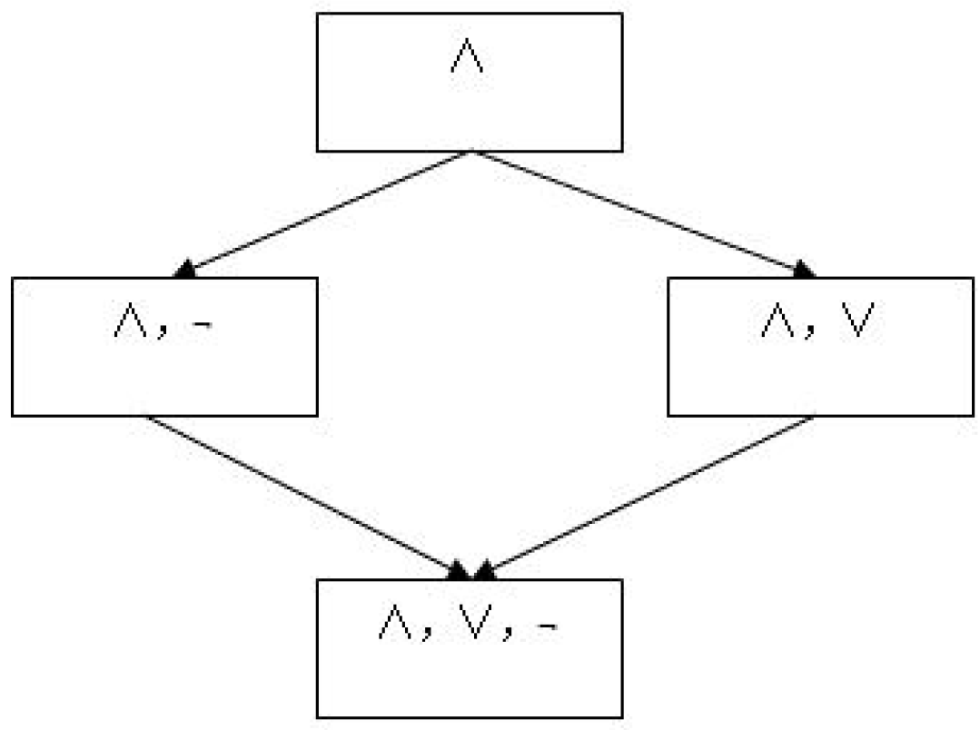
In summary, we know that both $X^{+}$ and $X^{▵}$ cannot serve as the upper $(\wedge ,\neg )$-approximate granule, and both $X^{-}$ and $X^{▿}$ cannot act as the lower $(\wedge ,\neg )$-approximate granule. Then, we conclude that FCA is not an effective tool for the $(\wedge ,\neg )$-approximate descriptions of granules.

5.2. $(\wedge ,\neg )$-Approximate Descriptions of Indefinable Granules Based on the Three-Way Concept Lattice

In this section, we present a method for $(\wedge ,\neg )$-approximate descriptions of indefinable granules based on the three-way concept lattice. Let $K=(G,M,I)$ be a formal context and $X\subseteq G$. If X is an extent of a three-way concept of K, then we call X a basic granule in the settings of three-way concept analysis.

In order to obtain simpler descriptions of granules, we first extend the notion of a minimal generator from a formal concept [39,47] to a three-way concept.

Definition 20. 

Let $K=(G,M,I)$ be a formal context and $(X,(A,B\left)\right)\in TL\left(K\right)$. If there are a subset E of A and a subset F of B such that $E^{\ast }\cap F^{\stackrel{-}{\ast }}=X$ and for any $(C,D)\le (E,F)$, $C^{\ast }\cap D^{\stackrel{-}{\ast }}\subset X$, then we call $(E,F)$ a minimal generator of $(X,(A,B\left)\right)$. Furthermore, if $(E,F)\le (S,T)\le (A,B)$, we call $(S,T)$ an intent reduct of $(X,(A,B\left)\right)$.

Proposition 13. 

Let $K=(G,M,I)$ be a formal context and $m,n\in M$. Then, both $(m^{\ast },(m^{\ast \ast },m^{\ast \stackrel{-}{\ast }}))$ and $(n^{\stackrel{-}{\ast }},(n^{\stackrel{-}{\ast }\ast },n^{\stackrel{-}{\ast }\stackrel{-}{\ast }}))$ are three-way concepts.

Proof. 

Let $X=m^{\ast }$ and $(A,B)=(m^{\ast \ast },m^{\ast \stackrel{-}{\ast }})$. On the one hand, we have $X^p=(m^{\ast \ast },m^{\ast \stackrel{-}{\ast }})=(A,B)$. On the other hand, as ${(A,B)}^q=m^{\ast \ast \ast }\cap m^{\ast \stackrel{-}{\ast }\stackrel{-}{\ast }}$, $m^{\ast \ast \ast }=m^{\ast }$ and $m^{\ast }\subseteq m^{\ast \stackrel{-}{\ast }\stackrel{-}{\ast }}$, we can obtain ${(A,B)}^q=m^{\ast \ast \ast }\cap m^{\ast \stackrel{-}{\ast }\stackrel{-}{\ast }}=m^{\ast }=X$. Then, $(m^{\ast },(m^{\ast \ast },m^{\ast \stackrel{-}{\ast }}))$ is a three-way concept. Moreover, the rest of the proposition can be proved likewise.    □

According to Proposition 13, we can define two types of attribute-induced three-way concepts.

Definition 21. 

Let $K=(G,M,I)$ be a formal context. If a three-way concept can be rewritten as $(m^{\ast },(m^{\ast \ast },m^{\ast \stackrel{-}{\ast }}))$ or $(n^{\stackrel{-}{\ast }},(n^{\stackrel{-}{\ast }\ast },n^{\stackrel{-}{\ast }\stackrel{-}{\ast }}))$, then this concept is referred to as an attribute-induced three-way concept. Moreover, we say that $(m^{\ast },(m^{\ast \ast },m^{\ast \stackrel{-}{\ast }}))$ is a type-I attribute-induced three-way concept and $(n^{\stackrel{-}{\ast }},(n^{\stackrel{-}{\ast }\ast },n^{\stackrel{-}{\ast }\stackrel{-}{\ast }}))$ is a type-II attribute-induced three-way concept.

Theorem 5 

([38]). Let $(X_1,(A_1,B_1))$ and $(X_2,(A_2,B_2))$ be two three-way concepts of a formal context $K=(G,M,I)$. Then, the infimum and supremum are given by:

$$(X_1,(A_1,B_1))\wedge (X_2,(A_2,B_2))=(X_1\cap X_2,{((A_1,B_1)\cup (A_2,B_2))}^{qp}),$$

$$(X_1,(A_1,B_1))\vee (X_2,(A_2,B_2))=({(X_1\cup X_2)}^{pq},(A_1,B_1)\cap (A_2,B_2)).$$

Theorem 6. 

Let $K=(G,M,I)$ be a formal context and $TL\left(K\right)$ be the three-way concept lattice of K. If a three-way concept $(X,(A,B\left)\right)$ of $TL\left(K\right)$ has only one upper neighbor, then it is an attribute-induced three-way concept.

Proof. 

As $(X,(A,B\left)\right)$ has only one upper neighbor, it follows that $(X,(A,B\left)\right)$ is a lower bound irreducible element. In other words, $(X,(A,B))\ne \bigwedge \{(X_i,(A_i,B_i))\in TL\left(K\right)|(X_i,(A_i,B_i))\ge (X,(A,B))\}$, which implies that $(X,(A,B))<\bigwedge \{(X_i,(A_i,B_i))\in TL\left(K\right)|(X_i,(A_i,B_i))\ge (X,(A,B))\}$. Let $\{(X_i,(A_i,B_i))\in TL\left(K\right)|(X_i,(A_i,B_i))\ge (X,(A,B))\}=\left\{(X_i,(A_i,B_i))\right|i\in I\}$. Then, according to Theorem 5, we have ${\displaystyle \underset{i\in I}{\bigwedge }}(X_i,(A_i,B_i))=({\displaystyle \bigcap _{i\in I}}{X}_i,{\left({\displaystyle \bigcup _{i\in I}}(A_i,B_i)\right)}^{qp})$. Therefore, we have $(A,B)>{\left({\displaystyle \bigcup _{i\in I}}(A_i,B_i)\right)}^{qp}>({\displaystyle \bigcup _{i\in I}}{A}_i,{\displaystyle \bigcup _{i\in I}}{B}_i)$, which means $(A-{\displaystyle \bigcup _{i\in I}}{A}_i)\ne Ø$ or $(B-{\displaystyle \bigcup _{i\in I}}{B}_i)\ne Ø$. If $A-{\displaystyle \bigcup _{i\in I}}{A}_i\ne Ø$, then there must exist an attribute $m\in A$ and $m\notin {\displaystyle \bigcup _{i\in I}}{A}_i$ such that $(X,(A,B\left)\right)$ can be rewritten as $(m^{\ast },(m^{\ast \ast },m^{\ast \stackrel{-}{\ast }}))$. If $B-{\displaystyle \bigcup _{i\in I}}{B}_i\ne Ø$, then there must exist an attribute $n\in B$ and $n\notin \bigcup _{i\in I}{B}_i$ such that $(X,(A,B\left)\right)$ can be rewritten as $(n^{\stackrel{-}{\ast }},(n^{\stackrel{-}{\ast }\ast },n^{\stackrel{-}{\ast }\stackrel{-}{\ast }}))$. To sum up, $(X,(A,B\left)\right)$ is an attribute-induced three-way concept.    □

Theorem 7. 

Let $K=(G,M,I)$ be a formal context and a three-way concept $(X,(A,B\left)\right)$ of $TL\left(K\right)$ has at least two upper neighbors ${(X_i,(A_i,B_i))}_{i\in I}$, where I is an index set and $\left|I\right|\ge 2$. If ${\displaystyle \bigcup _{i\in I}}(A_i,B_i)<(A,B)$, then $(X,(A,B\left)\right)$ is an attribute-induced three-way concept.

Proof. 

Since ${\displaystyle \bigcup _{i\in I}}(A_i,B_i)<(A,B)$, there exists $a\in A-{\displaystyle \bigcup _{i\in I}}{A}_i$ or $b\in B-{\displaystyle \bigcup _{i\in I}}{B}_i$. If there is $a\in A-{\displaystyle \bigcup _{i\in I}}{A}_i$, then this concept can be rewritten as $(a^{\ast },(a^{\ast \ast },a^{\ast \stackrel{-}{\ast }}))$. If there is $b\in B-{\displaystyle \bigcup _{i\in I}}{B}_i$, then this concept can be rewritten as $(b^{\stackrel{-}{\ast }},(b^{\stackrel{-}{\ast }\ast },b^{\stackrel{-}{\ast }\stackrel{-}{\ast }}))$. To sum up, the required conclusion is at hand.    □

Theorem 8. 

Let $K=(G,M,I)$ be a formal context and $TL\left(K\right)$ be the three-way concept lattice of K. $(m,Ø)$ is a minimal generator of $(m^{\ast },(m^{\ast \ast },m^{\ast \stackrel{-}{\ast }}))$, and $(Ø,n)$ is a minimal generator of $(n^{\stackrel{-}{\ast }},(n^{\stackrel{-}{\ast }\ast },n^{\stackrel{-}{\ast }\stackrel{-}{\ast }}))$.

Proof. 

According to the notions of an attribute-induced three-way concept and minimal generator of a three-way concept, the proof can be completed easily.    □

Definition 22. 

Let $(A,B)$ be a pair of two attribute sets. The simplification function carried on $(A,B)$ is defined as:

$$simpc(A,B)=(A-\{a\in A|\exists b\in B,a^{\ast }\supseteq b^{\stackrel{-}{\ast }}\},B-\{b\in B|\exists a\in A,a^{\ast }\subseteq b^{\stackrel{-}{\ast }}\}).$$

Definition 23. 

Let $(A,B)$ be a pair of two attribute sets. The simplification function carried on the first element and second element of $(A,B)$ are, respectively, defined as:

$$simp\left(A\right)=A-\{a_i\in A|\exists a_j\in A,a_i^{\ast }\supseteq a_j^{\ast }\}andsimp\left(B\right)=B-\{b_i\in B|\exists b_j\in B,b_i^{\stackrel{-}{\ast }}\supseteq b_j^{\stackrel{-}{\ast }}\}.$$

Definition 24. 

Let $(A,B)$ and $(C,D)$ be two pairs of attribute sets. The simplification-union function carried on $(A,B)$ and $(C,D)$ is defined as:

$$(A,B)\cup (C,D)=\left(simp\right(A\cup C),simp(B\cup D\left)\right).$$

Lemma 2. 

Let $(A,B)$ be a pair of two attribute sets and $simpc(A,B)=(E,F)$. Then, the following properties hold:

(i) ${\left(simp\left(A\right)\right)}^{\ast }=A^{\ast }$, ${\left(simp\left(B\right)\right)}^{\stackrel{-}{\ast }}=B^{\stackrel{-}{\ast }}$;

(ii) $A^{\ast }\cap B^{\stackrel{-}{\ast }}=E^{\ast }\cap F^{\stackrel{-}{\ast }}$.

Proof. 

(i) Without loss of generality, we assume that there exist two attributes $a_i$ and $a_j$ with $a_i^{\ast }\supseteq a_j^{\ast }$. Then, $a_i^{\ast }\cap a_j^{\ast }=a_j^{\ast }$, so a simple manipulation leads to the equation ${\left(simp\left(A\right)\right)}^{\ast }={\displaystyle \bigcup _{a\in simp\left(A\right)}}{a}^{\ast }={\displaystyle \bigcup _{a\in A-a_j}}{a}^{\ast }=A^{\ast }$. Moreover, ${\left(simp\left(B\right)\right)}^{\stackrel{-}{\ast }}=B^{\stackrel{-}{\ast }}$ can be proved likewise.

(ii) It follows immediately from Definition 24.    □

Lemma 3. 

In a three-way concept lattice, if a concept is not an attribute-induced three-way concept, then this concept has at least two upper neighbors.

Proof. 

It follows immediately from Theorem 6.    □

Lemma 4. 

In a three-way concept lattice, if a concept is not an attribute-induced three-way concept, then one of its intent reducts is the union of any two upper neighbors’ minimal generators.

Proof. 

Assume that $(X,(A,B\left)\right)$ is not an attribute-induced three-way concept. Lemma 3 indicates that $(X,(A,B\left)\right)$ has at least two upper neighbors and we denote them by ${(X_i,(A_i,B_i))}_{i\in I}$, where I is an index set. Moreover, we denote the minimal generator of $(X_i,(A_i,B_i))$ by $(E_i,F_i)$. Furthermore, $X={\displaystyle \bigcap _{i\in I}}{X}_i={\displaystyle \bigcap _{i\in I}}{(A_i,B_i)}^q={\displaystyle \bigcap _{i\in I}}{(E_i,F_i)}^q$. In addition, we take ${(A,B)}^q=X$ and ${\displaystyle \bigcap _{i\in I}}{(E_i,F_i)}^q={\left({\displaystyle \bigcup _{i\in I}}(E_i,F_i)\right)}^q$ into consideration, and then we have $X={(A,B)}^q={\left({\displaystyle \bigcup _{i\in I}}(E_i,F_i)\right)}^q$. Thence, the proof is completed.    □

Theorem 9. 

In a three-way concept lattice, if a concept is not an attribute-induced three-way concept, then one of its minimal generators is the simplification union of any two upper neighbors’ minimal generators.

Proof. 

This theorem follows immediately from Lemmas 2–4.    □

To sum up, according to Theorems 6 and 7, we can identify attribute-induced three-way concepts. Based on Theorems 8 and 9, we can obtain the minimal generators of each three-way concept. Algorithm 4 computes minimal generators of each three-way concept of a given three-way concept lattice.

Algorithm 4 Computing the minimal generator of each three-way concept.

Require: Three-way concept lattice $TL(G,M,I)$. Ensure: The minimal generator of each three-way concept.   1: Consider the three-way concept lattice $TL(G,M,I)$ as an undirected graph and traverse it downwards from the maximal three-way concept $(G,(Ø,Ø\left)\right)$ by using breadth-first search;   2: For the current visited concept   3:    If it fulfills Theorem 5 or Theorem 6   4:         Then, it is an attribute-induced three-way concept and obtains its minimal generator by using Theorem 7;   5:        Else compute its minimal generator by using Theorem 8;   6:    End If   7: End For   8: Return the minimal generators of all three-way concepts.

Let N be the number of concepts of $TL(G,M,I)$. In Algorithm 4, it is obvious that each three-way concept is visited just once, so the time complexity of this algorithm is $O\left(N\right)$.

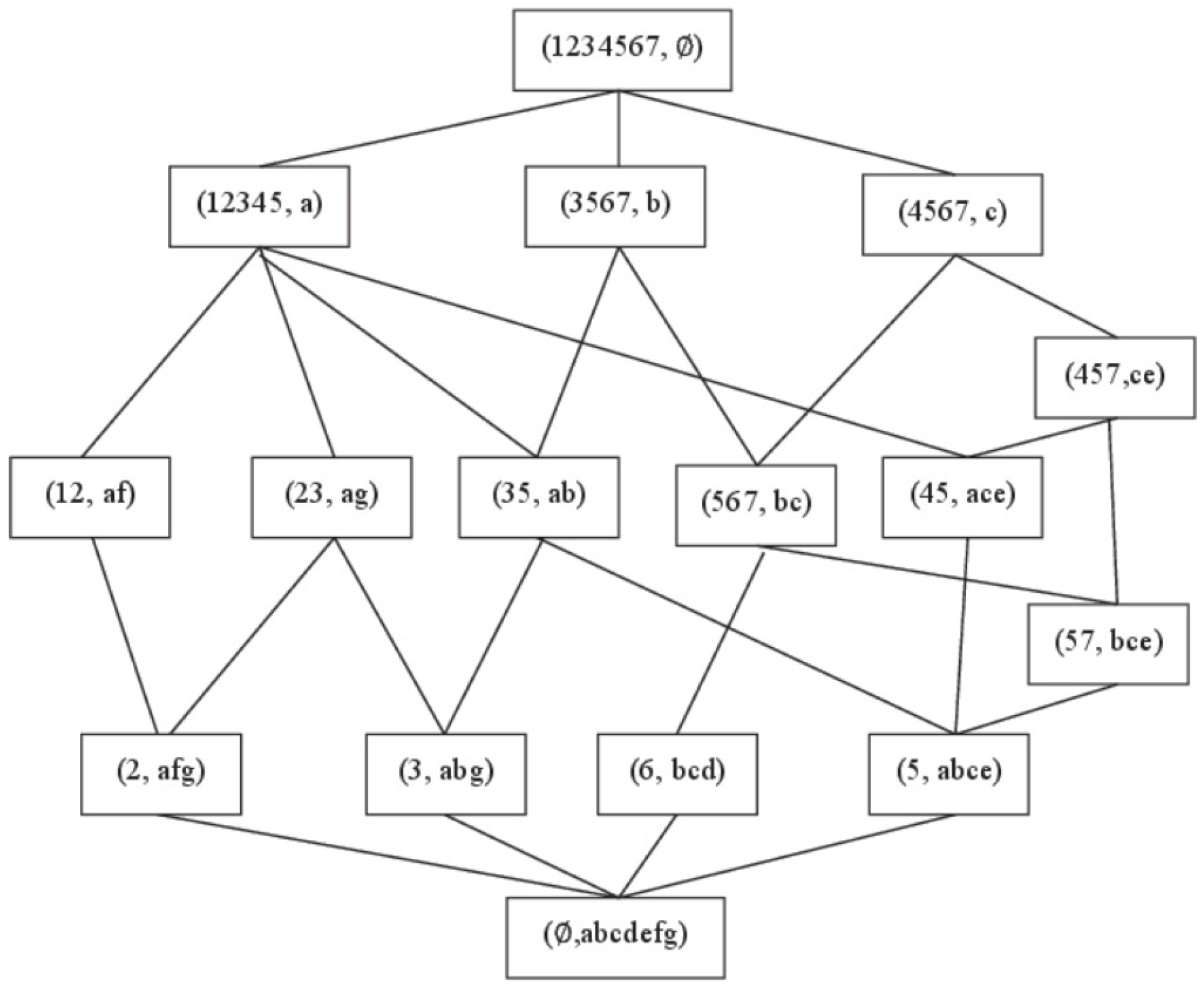
Example 8. 

Consider the formal context in Table 3. The three-way concept lattice is shown in Figure 4. Actually, each three-way concept corresponds to a $(\wedge ,\neg )$-definable granule. By using Algorithm 4, we obtain the minimal generators of all three-way concepts except $(G,(Ø,Ø\left)\right)$ and $(Ø,(M,M\left)\right)$. Then, we obtain their descriptions shown in

Table 4. Descriptions of $(\wedge ,\neg )$-definable granules.

Granules	Corresponding Concepts	Minimal Generators	Descriptions
$\left\{1236\right\}$	$(1236,(Ø,e\left)\right)$	$(Ø,e)$	$\neg e$
$\left\{123457\right\}$	$(123457,(Ø,d\left)\right)$	$(Ø,d)$	$\neg d$
$\left\{34567\right\}$	$(34567,(Ø,f\left)\right)$	$(Ø,f)$	$\neg f$
$\left\{14567\right\}$	$(14567,(Ø,g\left)\right)$	$(Ø,g)$	$\neg g$
$\left\{12345\right\}$	$(12345,(a,d\left)\right)$	$(a,Ø)$	a
$\left\{1457\right\}$	$(1457,(Ø,dg\left)\right)$	$(Ø,dg)$	$\neg d\wedge \neg g$
$\left\{3457\right\}$	$(3456,(Ø,df\left)\right)$	$(Ø,df)$	$\neg d\wedge \neg f$
$\left\{3567\right\}$	$(3567,(b,f\left)\right)$	$(b,Ø)$	b
$\left\{4567\right\}$	$(4567,(c,fg\left)\right)$	$(c,Ø)$,$(Ø,fg)$	c,$\neg f\wedge \neg g$
$\left\{123\right\}$	$(123,(a,cde\left)\right)$	$(a,e)$,$(Ø,c)$	$a\wedge e$, $\neg c$
$\left\{124\right\}$	$(124,(a,bd\left)\right)$	$(Ø,b)$	$\neg b$
$\left\{145\right\}$	$(145,(a,dg\left)\right)$	$(a,dg)$	$a\wedge \neg d\wedge \neg g$
$\left\{345\right\}$	$(345,(a,df\left)\right)$	$(a,df)$	$a\wedge \neg d\wedge \neg f$
$\left\{357\right\}$	$(357,(b,df\left)\right)$	$(b,d)$	$b\wedge \neg d$
$\left\{457\right\}$	$(457,(ce,dfg\left)\right)$	$(Ø,dfg)$,$(c,dg)$,$(c,df)$	$\neg d\wedge \neg f\wedge \neg g$,$c\wedge \neg d\wedge \neg g$,$c\wedge \neg d\wedge \neg f$
$\left\{567\right\}$	$(567,(bc,fg\left)\right)$	$(bc,Ø)$,$(b,fg)$	$b\wedge c$,$b\wedge \neg f\wedge \neg g$
$\left\{16\right\}$	$(16,(Ø,eg\left)\right)$	$(Ø,eg)$	$\neg e\wedge \neg g$
$\left\{36\right\}$	$(36,(b,ef\left)\right)$	$(b,e)$	$b\wedge \neg e$
$\left\{23\right\}$	$(23,(ag,cde\left)\right)$	$(g,Ø)$	g
$\left\{12\right\}$	$(12,(af,bcde\left)\right)$	$(f,Ø)$	f
$\left\{14\right\}$	$(14,(a,bdg\left)\right)$	$(Ø,bg)$	$\neg b\wedge \neg g$
$\left\{45\right\}$	$(45,(ace,dfg\left)\right)$	$(a,dfg)$	$a\wedge \neg d\wedge \neg f\wedge \neg g$
$\left\{35\right\}$	$(35,(ab,df\left)\right)$	$(ab,Ø)$	$a\wedge b$
$\left\{57\right\}$	$(57,(bce,dfg\left)\right)$	$(bc,d)$,$(b,dg)$	$b\wedge c\wedge \neg d$, $b\wedge \neg d\wedge \neg g$
$\left\{67\right\}$	$(67,(bc,afg\left)\right)$	$(Ø,a)$	$\neg a$
$\left\{1\right\}$	$(1,(af,bcdeg\left)\right)$	$(Ø,beg)$	$\neg b\wedge \neg e\wedge \neg g$
$\left\{2\right\}$	$(2,(afg,bcde\left)\right)$	$(fg,Ø)$	$f\wedge g$
$\left\{3\right\}$	$(3,(abg,cdef\left)\right)$	$(ab,e)$,$(bg,Ø)$	$a\wedge b\wedge \neg e$,$b\wedge g$
$\left\{4\right\}$	$(4,(ace,bdfg\left)\right)$	$(Ø,bdfg)$	$\neg b\wedge \neg d\wedge \neg f\wedge \neg g$
$\left\{5\right\}$	$(5,(abce,dfg\left)\right)$	$(abc,Ø)$,$(ab,g)$	$a\wedge b\wedge c$, $a\wedge b\wedge \neg g$
$\left\{6\right\}$	$(6,(bcd,aefg\left)\right)$	$(Ø,ae)$	$\neg a\wedge \neg e$
$\left\{7\right\}$	$(7,(bce,adfg\left)\right)$	$(Ø,ad)$	$\neg a\wedge \neg d$

.

Definition 25. 

Let $K=(G,M,I)$ be a formal context and $X\subseteq G$ be a granule. If there exist two three-way concepts $(X_1,(A_1,B_1))$ and $(X_2,(A_2,B_2))$ such that $X_1\subseteq X\subseteq X_2$, we say that X is approximately $(\wedge ,\neg )$-definable.

Theorem 10. 

All granules are approximately $(\wedge ,\neg )$-definable.

Proof. 

This theorem can be proved similarly to that of Theorem 3.    □

Definition 26. 

Let $K=(G,M,I)$ be a formal context and $X\subseteq G$ be a granule. $C\in TL\left(K\right)$ is called the upper $(\wedge ,\neg )$-approximate three-way concept of X if $X\subseteq ext\left(C\right)$ and there does not exist $D\in TL\left(K\right)$ such that $X\subseteq ext\left(D\right)\subset ext\left(C\right)$. Correspondingly, $C\in TL\left(K\right)$ is called the lower $(\wedge ,\neg )$-approximate three-way concept of X if $X\supseteq ext\left(C\right)$ and there does not exist $D\in TL\left(K\right)$ such that $X\supseteq ext\left(D\right)\supset ext\left(C\right)$.

Similar to the case in Algorithm 1, here both the upper and lower $(\wedge ,\neg )$-approximate three-way concepts of X may not be unique. According to Definitions 2 and 26, there exists an upper $(\wedge ,\neg )$-approximate three-way concept $(X_1,(A_1,B_1))$ of X such that

$\alpha \left(\left({\displaystyle \underset{r\in A_1}{\bigwedge }}r\right)\wedge \left({\displaystyle \underset{s\in B_1}{\bigwedge }}\neg s\right),X\right)=1$ and $\beta (\phi ,X)$ reaches the biggest value. Similarly, there exists a lower $(\wedge ,\neg )$-approximate three-way concept $(X_2,(A_2,B_2))$ of X such that

$\beta \left(\left({\displaystyle \underset{r\in A_2}{\bigwedge }}r\right)\wedge \left({\displaystyle \underset{s\in B_2}{\bigwedge }}\neg s\right),X\right)=1$ and $\alpha (\phi ,X)$ reaches the biggest value. Actually, $X_1$ is the upper $(\wedge ,\neg )$-approximate granule of X and $X_2$ is the lower $(\wedge ,\neg )$-approximate granule of X. Then, based on Definitions 5 and 6, we can use the upper and lower $(\wedge ,\neg )$-approximate three-way concepts of X to construct the $\alpha$-prior approximate optimal description, the $\beta$-prior approximate optimal description, and the $(\wedge ,\neg )$-approximate description $d^{\ast }\left(X\right)$ of X. The detailed procedure is shown in Algorithm 5.

Algorithm 5 Computing the $(\wedge ,\neg )$-approximate description of a granule.

Require: Three-way concept lattice $TL(G,M,I)$ and a granule $X\subseteq G$. Ensure: If X is $(\wedge ,\neg )$-definable, then this algorithm outputs the description $d\left(X\right)$ of X; otherwise, this algorithm outputs the $(\wedge ,\neg )$-approximate description $d^{\ast }\left(X\right)$ of X.   1: If there exists a three-way concept $(X,(A,B\left)\right)$   2:    Then Return “X is $(\wedge ,\neg )$-definable” and $d\left(X\right)=\left({\displaystyle \underset{r\in R}{\bigwedge }}r\right)\wedge \left({\displaystyle \underset{s\in S}{\bigwedge }}\neg s\right)$, where $(R,S)$ is the minimal generator of $(X,(A,B\left)\right)$;   3:    Else find the upper approximate three-way concept $(X_u,(A_u,B_u))$ and lower approximate three-way concept $(X_l,(A_l,B_l))$ of X;   4:        Based on $(X_u,(A_u,B_u))$, we derive $d^{\alpha \ast }\left(X\right)=\left({\displaystyle \underset{r\in R_u}{\bigwedge }}r\right)\wedge \left({\displaystyle \underset{s\in S_u}{\bigwedge }}\neg s\right)$, where $(R_u,S_u)$ is the minimal generator of $(X_u,(A_u,B_u))$;   5:       Based on $(X_l,(A_l,B_l))$, we derive $d^{\beta \ast }\left(X\right)=\left({\displaystyle \underset{r\in R_l}{\bigwedge }}r\right)\wedge \left({\displaystyle \underset{s\in S_l}{\bigwedge }}\neg s\right)$, where $(R_l,S_l)$ is the minimal generator of $(X_l,(A_l,B_l))$;   6:       Return $d^{\ast }\left(X\right)=[d^{\beta \ast }\left(X\right),d^{\alpha \ast }\left(X\right)]$.   7:    End Else   8: End If

Note that the minimal generator of a concept is often more concise to describe a granule than the intent of the concept [39]. So, Algorithm 5 adopts such a technique as usual.

The time complexity of Algorithm 5 depends on the cost of finding the upper and lower approximate three-way concepts and the calculation of minimal generators. Apparently, in order to find the upper and lower $(\wedge ,\neg )$-approximate three-way concepts, the number of visited concepts is less than N. Moreover, when computing minimal generators, the number of visited concepts is still less than N. So, the time complexity of Algorithm 5 is $O\left(N\right)$.

Example 9. 

Consider the formal context in Table 3. Let $X=\{1,2,3,4\}$. It is easy to check that X is a $(\wedge ,\neg )$-indefinable granule.

Then, by using Algorithm 5, we can compute its $(\wedge ,\neg )$-approximate description in three steps:

(i) we obtain the upper $(\wedge ,\neg )$-approximate three-way concept of X and the result is $(12345,(a,d\left)\right)$;

(ii) we obtain the lower $(\wedge ,\neg )$-approximate thee-way concept of X and the result is $(123,(a,cde\left)\right)$ or $(124,(a,bd\left)\right)$;

(iii) we derive the approximate description of X and the result is $d^{\ast }\left(X\right)=[a\wedge \neg e,a]$ or $[\neg c,a]$ or $[\neg b,a]$ with $Acc\left(d^{\ast }\left(X\right)\right)=0.6$.

5.3. $(\wedge ,\vee ,\neg )$-Approximate Descriptions of Indefinable Granules Based on a Three-Way Concept Lattice

In this section, we propose a method for $(\wedge ,\vee ,\neg )$-approximate descriptions of indefinable granules based on a three-way concept lattice.

Proposition 14. 

Let $K=(G,M,I)$ be a formal context and $X\subseteq G$ be a granule. If there exist $x\in X$ and $y\in G-X$ such that $x^p=y^p$, then X is $(\wedge ,\vee ,\neg )$-indefinable; otherwise, X is $(\wedge ,\vee ,\neg )$-definable.

Proof. 

If there exist $x\in X$ and $y\in G-X$ such that $x^p=y^p$, then we cannot distinguish x from y by using both positive and negative attributes. By the definition of an $(\wedge ,\vee ,\neg )$-indefinable granule, it follows that X is $(\wedge ,\vee ,\neg )$-indefinable. Otherwise, we always have a description $d\left(X\right)={\displaystyle \underset{x\in X}{\bigvee }}\left(\left({\displaystyle \underset{a\in x^{\ast }}{\bigwedge }}a\right)\wedge \left({\displaystyle \underset{b\in X^{\stackrel{-}{\ast }}}{\bigwedge }}\neg b\right)\right)$. Hence, X is $(\wedge ,\vee ,\neg )$-definable.    □

Definition 27. 

Let $K=(G,M,I)$ be a formal context. For any $X\in 2^G$, a pair of operators $\boxminus ,⊞:2^G\to 2^G$ are defined, respectively, as:

$$X^{\boxminus }=\left\{x\right|x\in X,\neg \exists y\in G-X,y^p=x^p\}and X^{⊞}=X\cup X^{\boxminus }.$$

Based on Proposition 14 and Definition 27, we immediately obtain the following Corollaries 4, 5, and 6.

Corollary 4. 

Let X be a granule. Then, both $X^{\boxminus }$ and $X^{⊞}$ are $(\wedge ,\vee ,\neg )$-definable.

Corollary 5. 

Let X be a granule. If $X=X^{\boxminus }$ or $X=X^{⊞}$, then X is $(\wedge ,\vee ,\neg )$-definable.

Corollary 6. 

Let X be a granule. $X^{\boxminus }$ is the lower $(\wedge ,\vee ,\neg )$-approximate granule of X and $X^{⊞}$ is the upper $(\wedge ,\vee ,\neg )$-approximate granule of X.

Definition 28. 

Let $K=(G,M,I)$ be a formal context and $X\subseteq G$ be a granule. If there exist two $(\wedge ,\vee ,\neg )$-definable granules $X_1$ and $X_2$ such that $X_1\subseteq X\subseteq X_2$, we say that X is approximately $(\wedge ,\vee ,\neg )$-definable.

Theorem 11. 

All granules are approximately $(\wedge ,\vee ,\neg )$-definable.

Proof. 

Let $K=(G,M,I)$ be a formal context and $X\subseteq G$ be a granule. First, we can always derive $X^{⊞}$ and $X^{\boxminus }$. Moreover, Corollary 4 states that both $X^{⊞}$ and $X^{\boxminus }$ are $(\wedge ,\vee ,\neg )$-definable. Then, it follows that X is approximately $(\wedge ,\vee ,\neg )$-definable.    □

For a given $(\wedge ,\vee ,\neg )$-definable granule X, we have $d\left(X\right)={\displaystyle \underset{x\in X}{\bigvee }}\left(\left({\displaystyle \underset{s\in x^{\ast }}{\bigwedge }}s\right)\wedge \right.$$\left.\left({\displaystyle \underset{t\in (M-x^{\ast })}{\bigwedge }}\neg t\right)\right)$. However, it needs time to obtain the simplest form of $d\left(X\right)$ by performing logical operations. To solve this problem, we resort to a three-way concept lattice.

By using Algorithm 6, we can calculate the descriptions of $(\wedge ,\vee ,\neg )$-definable granules.

Algorithm 6 Computing the description of a $(\wedge ,\vee ,\neg )$-definable granule.

Require: Three-way concept lattice $TL(G,M,I)$ and a $(\wedge ,\vee ,\neg )$-definable granule $X\subseteq G$. Ensure: This algorithm outputs the description of X.   1: Represent X by its elements $X_1=\left\{x_1\right\}$, $X_2=\left\{x_2\right\}$, ⋯, $X_n=\left\{x_n\right\}$;   2: Let $S=\{X_1,X_2,\cdots ,X_n\}$;   3: Consider the three-way concept lattice $TL(G,M,I)$ as an undirected graph and traverse it upwards from the minimal three-way concept $(Ø,(M,M\left)\right)$ by using breadth-first search;   4: If there exist subsets $X_i\subseteq X$$(t\in T)$ and a three-way concept $(Y,(Y^{\ast },Y^{\stackrel{-}{\ast }}))$ such that ${\displaystyle \bigcup _{t\in T}}{X}_i=Y$   5:    Then delete $X_i\subseteq X$$(t\in T)$ from S and add Y into S;   6: Denote the updated result of S as $\{S_i\mid i\in I\}$;   7: $d\left(X\right)={\displaystyle \underset{i\in I}{\bigvee }}d\left(S_i\right)$, where $d\left(S_i\right)$ is the $(\wedge ,\neg )$-description of $S_i$;   8: Return $d\left(X\right)$.

Example 10. 

Consider the formal context in Table 3. Let $X=\{1,3,5,6,7\}$. By using Algorithm 6, we obtain the description of X by combining the $(\wedge ,\neg )$-descriptions of the granules $\left\{1\right\}$, $\left\{3\right\}$ and $\{5,6,7\}$. That is, $d\left(X\right)=(\neg b\wedge \neg e\wedge \neg g)\vee (b\wedge g)\vee (b\wedge c)$.

Similar to the case in Algorithm 3, there exists an upper $(\wedge ,\vee ,\neg )$-approximate granule $X^{⊞}$ of X such that $\alpha (d\left(X^{⊞}\right),X)=1$ and $\beta (\phi ,X)$ reaches the biggest value. Similarly, there exists a lower $(\wedge ,\vee ,\neg )$-approximate granule $X^{\boxminus }$ of X such that $\beta (d\left(X^{-}\right),X)=1$ and $\alpha (\phi ,X)$ reaches the biggest value. Then, based on Definitions 5 and 6, we can use the upper and lower $(\wedge ,\vee ,\neg )$-approximate granules of X to construct the $\alpha$-prior approximate optimal description, the $\beta$-prior approximate optimal description, and the $(\wedge ,\vee ,\neg )$-approximate description $d^{\ast }\left(X\right)$ of X. The detailed procedure is shown in Algorithm 7. In addition, the time complexity of Algorithm 7 is $O\left(L\right)$.

Algorithm 7 Computing the $(\wedge ,\vee ,\neg )$-approximate description of a granule.

Require: Three-way concept lattice $TL(G,M,I)$ and a granule $X\subseteq G$. Ensure: If X is $(\wedge ,\vee ,\neg )$-definable, then this algorithm outputs the description $d\left(X\right)$ of X; otherwise, this algorithm outputs the $(\wedge ,\vee ,\neg )$-approximate description $d^{\ast }\left(X\right)$ of X.   1: Compute $X^{⊞}$ and $X^{\boxminus }$;   2: If  $X^{⊞}=X^{\boxminus }$   3:    Then X is $(\wedge ,\vee ,\neg )$-definable and compute its description $d\left(X\right)$ by calling Algorithm 6;   4:           Return $d\left(X\right)$;   5:    Else compute the descriptions of $X^{⊞}$ and $X^{\boxminus }$ by calling Algorithm 6;   6:           Return $d^{\ast }\left(X\right)=[d\left(X^{\boxminus }\right),d\left(X^{⊞}\right)]$.   7: End If

Example 11. 

Consider the formal context in Table 3. Let $X=\{1,3,5,6,7\}$. If we add a new object 8 with the same description as that of object 3 into X, then X changes to be a $(\wedge ,\vee ,\neg )$-indefinable granule. According to Algorithm 7, we obtain the upper and lower $(\wedge ,\vee ,\neg )$-approximate granules $X^{⊞}=\{1,3,5,6,7,8\}$ and $X^{\boxminus }=\{1,5,6,7\}$, respectively. And then, we have the $(\wedge ,\vee ,\neg )$-approximate description

$$d^{\ast }\left(X\right)=[d\left(X^{\boxminus }\right),d\left(X^{⊞}\right)]=[(\neg b\wedge \neg e\wedge \neg g)\vee (b\wedge c),(\neg b\wedge \neg e\wedge \neg g)\vee (b\wedge g)\vee (b\wedge c)]$$

with

$$Acc\left(d^{\ast }\left(X\right)\right)={\displaystyle \frac{\left|m\right(d^{\beta \ast }\left(X\right)\left)\right|}{\left|m\right(d^{\alpha \ast }\left(X\right)\left)\right|}}={\displaystyle \frac{\left|\right\{1,5,6,7\left\}\right|}{\left|\right\{1,3,5,6,7,8\left\}\right|}}={\displaystyle \frac{2}{3}}.$$

6. A Case Study and Experimental Analysis

Example 12. 

In a science and education film called “Biology and Water” in Hungary, there are eight species of organisms, namely, grasshoppers (1), fish (2), frogs (3), dogs (4), aquatic plants (5), reeds (6), beans (7), and corn (8). At the same time, this movie emphasizes nine biological attributes, namely, a (requiring water), b (living in water), c (living on land), d (having chlorophyll), e (dicotyledonous), f (having a single cotyledon), g (being able to move), h (having limbs), and i (breastfeeding). The formal context of these organisms is shown in

Table 5. Formal context “Biology and Water”.

	a	b	c	d	e	f	g	h	i
1	∗	∗					∗
2	∗	∗					∗	∗
3	∗	∗	∗				∗	∗
4	∗		∗				∗	∗	∗
5	∗	∗		∗		∗
6	∗	∗	∗	∗		∗
7	∗		∗	∗	∗
8	∗		∗	∗		∗

[12].

By using FCA, we can obtain the concept lattice $L\left(K\right)$, which has 19 formal concepts. In other words, there are 19 basic granules (∧-definable granules) in the settings of classical formal concept analysis, and these basic granules are described with ∧-based language. For instance, $\{1,2,3\}$ is an extent of $\left(\right\{1,2,3\},\{a,b,g\left\}\right)$, and thus $\{1,2,3\}$ is a basic and ∧-definable granule with a description $a\wedge b\wedge g$, which means that they need water, live in water, and have the ability to move. Based on ∧-definable granules, we can obtain $(\wedge ,\vee )$-definable granules.

Based on three-way concept analysis, we can derive the three-way concept lattice $TL\left(K\right)$, which has 44 three-way concepts. Therefore, we can obtain 44 basic granules ($(\wedge ,\neg )$-definable granules) in the settings of three-way concept analysis, and describe these basic granules with $(\wedge ,\neg )$-based language. For instance, $\{3,6,8\}$ is an extent of $\left(\right\{3,6,8\},(\left\{c\right\},\{e,i\}\left)\right)$, and thus $\{3,6,8\}$ is a basic and $(\wedge ,\neg )$-definable granule with a description $c\wedge \neg e\wedge \neg i$, which means that they live on land, and are not dicotyledonous and breastfeeding. Based on $(\wedge ,\neg )$-definable granules, we can obtain $\{\wedge ,\vee ,\neg \}$-definable granules.

By comparing the FCA and three-way concept analysis-based method, the latter can derive more basic granules, and thus can improve the description accuracy. In what follows, we test this based on experiments by randomly generated formal contexts.

In the experiments, the number of basic granules and the time consumptions to acquire them are investigated. It should be pointed out that the time consumption contains the process of building the concept lattices. The formal contexts $(G,M,I)$ are generated by fixing the fill ratio $r={\displaystyle \frac{\left|I(x,y)\mid I(x,y)=1,x\in G,y\in M\right|}{\left|G\right|\left|M\right|}}=0.5$ and $\left|G\right|=\left|M\right|$ while changing $\left|G\right|$ and $\left|M\right|$. The experimental results in terms of the number of concepts and time consumptions are shown in Figure 5 and Figure 6, which reveals that the three-way concept analysis-based method can derive more basic granules, and the FCA-based method needs less time consumption.

7. Conclusions

In this section, we draw some conclusions to show the main contributions of our paper and give an outlook for further study.

(i) A brief summary of our study

In this study, the approximate description of granules has been investigated. More specifically, approximate description logic has been introduced and we have approximated indefinable granules by using a couple of descriptions of two definable granules, that is the $\alpha$-prior optimal approximate description and the $\beta$-prior optimal approximate description. By using this idea throughout our study, at first, we explored the ∧-approximate descriptions of granules based on FCA, and then we presented the $(\wedge ,\vee )$-approximate descriptions of granules by using object pictorial diagrams. After that, some necessary discussions were presented to show the ineffectiveness of FCA until negative attributes are taken into consideration. Therefore, we have resorted to 3WCA instead of FCA to characterize granules both in positive and negative perspectives. Concretely, we presented $(\wedge ,\neg )$-approximate descriptions and $(\wedge ,\vee ,\neg )$-approximate descriptions of granules based on a three-way concept lattice, respectively.

(ii) The differences and similarities between our study and existing ones

Formal concept analysis and rough set analysis are two related theories used in granular computing. By incorporating these two theories, Yao proposed rough-set concept analysis in which $RS$-definable concepts were studied [16]. In some sense, according to the mathematical logic used in rough-set concept analysis, rough-set definable concepts are actually attribute concepts under the framework of the object-oriented concept lattice. So, given a rough-set definable granule, the description of the granule can be obtained by consulting the intent of its corresponding object-oriented concept.

More precisely, let X be a rough-set definable granule. Then, the description of X is

$$d\left(X\right)=\underset{b\in B}{\bigwedge }b,$$

where $B=\{b\in AT\mid b^{\ast }\subseteq X\}$.

However, in our studies, common attribute analysis is used. That is, if X is a ∧-definable granule, then the description of X is

$$d\left(X\right)=\underset{b\in B}{\bigwedge }b,$$

where $B=\{b\in M\mid \forall x\in X,xIb\}$.

Moreover, in our studies, a more flexible logic has been adopted which contains the connectives ∧, ∨, and ¬. The existing studies, including Yao’s work [16], have provided a granule description for basic granules. Putting it simply, if a granule X is an extent of a formal concept, then X is a basic granule. A basic granule X can be described by connecting the attribute contained in $X^{\ast }$, i.e., $a_1\wedge a_2\wedge \cdots \wedge a_i$, where $a_1,a_2,\cdots ,a_n\in X^{\ast }$. Then, it is clear that only the connective ∧ is adopted to construct a formula to describe a granule. But in this study, we consider using the connectives ∧, ∨, and ¬ to build more powerful descriptions.

In addition, in [39], we gave the descriptions of ∧-definable granules based on FCA, and presented the problem of describing indefinable granules. In this paper, we have systematically investigated the approximate descriptions of four important types of indefinable granules, i.e., ∧-indefinable granules, $(\wedge ,\vee )$-indefinable granules, $(\wedge ,\neg )$-indefinable granules, and $(\wedge ,\vee ,\neg )$-indefinable granules. So, this study can not only be regarded as a continuation of our previous research, but also brings us a more deep understanding of indefinable granules.

(iii) An outlook for further study

Note that the aim of this paper is to give an approximate description method for the granules of complete data. But in most circumstances, we have to deal with the granules of incomplete data. So, how to approximately describe the granules of incomplete data is a challenging and important issue. In addition, granule description can serve as the basic mathematical model for a variety of applications. As an instance, in conflict analysis, the allied, conflict, and neutral cliques are actually granules with different features [48]. Approximate description of these cliques is necessary on many occasions, especially in vague and uncertain settings. More efforts are needed for these problems.