Improved Hadamard Decomposition and Its Application in Data Compression in New-Type Power Systems

Abstract

The proliferation of renewable energy sources, flexible loads, and advanced measurement devices in new-type power systems has led to an unprecedented surge in power signal data, posing significant challenges for data management and analysis. This paper presents an improved Hadamard decomposition framework for efficient power signal compression, specifically targeting voltage and current signals which constitute foundational measurements in power systems. First, we establish theoretical guarantees for decomposition uniqueness through orthogonality and non-negativity constraints, thereby ensuring consistent and reproducible signal reconstruction, which is critical for power system applications. Second, we develop an enhanced gradient descent algorithm incorporating adaptive regularization and early stopping mechanisms, achieving superior convergence performance in optimizing the Hadamard approximation. The experimental results with simulated and field data demonstrate that the proposed scheme significantly reduces data volume while maintaining critical features in the restored data. In addition, compared with other existing compression methods, this scheme exhibits remarkable advantages in compression efficiency and reconstruction accuracy, particularly in capturing transient characteristics critical for power quality analysis.

1. Introduction

The need for the decarbonization and more efficient use of energy resources worldwide is driving a radical evolution in power systems. The increasing penetration of renewable energy sources, coupled with the integration of flexible loads and energy storage systems, has transformed traditional power grids into more complex and dynamic new-type power systems [1,2]. This transformation necessitates sophisticated monitoring and control infrastructure to ensure system stability and reliability. In new-type power systems, advanced measurement devices have been widely deployed at different voltage levels, including Phasor Measurement Units (PMUs) for high-voltage networks and Smart Meters (SMs) for household-level monitoring. For instance, in the USA, the number of installed PMUs is expected to exceed 1170 devices between 2018 and 2025, while the deployment of SMs is growing at an annual rate of 8.0% [3,4,5].

The proliferation of measurement devices generates an unprecedented volume of power system data, such as power quality disturbance (PQD) data, which are crucial for system operation and analysis. These data provide essential insights into system performance, fault detection, and operational stability, playing a vital role in ensuring the safe and reliable operation of modern power systems. The integration of renewable energy and flexible loads in new-type power systems introduces more complex and dynamic signal patterns, demanding compression methods that can effectively preserve both steady-state and transient features while achieving higher compression ratios for distributed data processing. However, the sheer volume of collected data poses significant challenges for data storage, transmission, and real-time processing capabilities. For example, a typical power quality monitoring system may generate several gigabytes of data daily, creating substantial demands on communication bandwidth and storage infrastructure. Therefore, developing efficient data compression methods has become increasingly critical for managing the volume and complexity of power system measurements while maintaining the integrity of essential information for subsequent analysis and decision-making processes [6,7].

1.1. Related Work

A variety of methods have been proposed and employed to address data compression, which are broadly classified into two categories: lossless compression methods and lossy compression methods [8]. Lossless compression methods usually employ data statistics and perform efficient bitwise encoding. Therefore, data can be reconstructed without any loss of information. Commonly used lossless compression methods include Huffman coding, Lempel–Ziv coding, and Golomb coding [9,10,11,12]. Ref. [9] proposed two real-time data compression schemes for ocean monitoring buoys: ERCS-Lossless and ERCS-Lossy-Flag, where ERCS-Lossless used Golomb–Rice coding for lossless compression, achieving a 47.40% average compression rate. Ref. [10] presented a model-free lossless data compression method known as lossless coding considering precision for time-series data in smart grids. This method used differential coding, XOR coding, and variable length coding to encode data points relative to their immediate predecessors. Ref. [11] proposed a multi-stage hybrid coding scheme for efficient lossless compression of high-density synchrophasor and point-on-wave data, including an improved-time-series-special compression method for frequency data, a delta-difference Huffman method for phase angle data, and a cyclical high-order delta modulation method for point-on-wave data. In summary, lossless methods focus on scenarios with high precision requirements, but the compression ratio (CR) is usually low. Therefore, it is not necessary to apply lossless methods in all cases. For example, it is more suitable to use lossy methods to compress PQD data, as there is such a vast amount of data that it is acceptable to discard some details.

Lossy compression methods sacrifice accuracy for a larger CR, and a small loss of information is tolerated [13,14]. Several interesting works on power data compression have been published in recent years, including coverage of methods such as principal component analysis (PCA) [15], singular value decomposition (SVD) [16,17,18], wavelet transform (WT) [19,20,21], and machine learning methods [22,23]. In [15], a two-stage compression technique for PMUs data was introduced, addressing the challenge of handling large volumes of synchrophasor and point-on-wave data. Ref. [18] utilized optimal SVD to reduce the number of singular values in the transmission process, and employed various intelligent optimization methods to determine the optimal values for elimination, enhancing CR and data quality. Ref. [19] proposed models for dynamic bit allocation based on adaptive and fixed spectral envelope estimation for transformed coefficients, using WT for bit allocation and entropy coding for coefficient vector encoding. While these methods have shown acceptable results, there is still a need for compression methods that can achieve larger CRs while preserving more essential characteristics. In this context, Hadamard decomposition presents promising results.

Hadamard decomposition is used to break down a signal or matrix into components by applying the element-wise Hadamard product between two or more matrices [24,25,26,27,28]. Unlike SVD, which decomposes a matrix into orthogonal matrices and a diagonal matrix, or PCA, which identifies principal components, Hadamard decomposition focuses on element-wise multiplicative relationships. Ref. [25] discussed a general framework for reducing the number of trainable model parameters in deep learning networks by decomposing linear operators as a product of sums of simpler linear operators. In [27], the Hadamard product allowed for the low-rank communication-efficient parameterization, leading to a flexible tradeoff between the number of trainable parameters and network accuracy. In compression, Hadamard decomposition enables the breakdown of large datasets into smaller, element-wise compressed parts. A mixed decomposition model of matrices which combined the Hadamard decomposition with the SVD was described in [28], where the potential multiplication structures of the dataset were discovered.

Based on the above analysis, Hadamard decomposition presents promising potential for power system data compression due to its ability to transform high-rank matrices into products of low-rank matrices. However, several critical challenges limit its practical application in power systems. Firstly, the non-unique decomposition results significantly hinder reproducibility and reliability, making it difficult to ensure consistent data reconstruction. Secondly, traditional optimization methods for Hadamard decomposition often suffer from slow convergence and instability. These limitations necessitate fundamental improvements to both the decomposition framework and optimization process.

1.2. Key Contributions

This paper proposes an enhanced Hadamard decomposition framework specifically designed for power signal compression, with the following key contributions.

• Uniqueness in Decomposition: We achieve uniqueness in Hadamard decomposition by imposing orthogonality and non-negativity constraints on the decomposed matrices. This theoretical advancement ensures consistent and reproducible signal reconstruction, which is essential for power system applications.
• Enhanced Gradient Descent Algorithm: We develop an enhanced gradient descent algorithm incorporating adaptive regularization and early stopping mechanisms. This algorithmic improvement significantly accelerates convergence and improves computational efficiency in optimizing the Hadamard approximation, making it practical for real-time power system applications.
• Novel Compression Scheme: We design a novel compression scheme for current and voltage data compression of power systems based on the improved Hadamard decomposition. This scheme demonstrates superior performance in both compression efficiency and feature preservation, particularly in capturing transient characteristics critical for power quality analysis.

The remainder of this paper is organized as follows. Section 2 introduces the Hadamard decomposition and provides proof of the uniqueness. The enhanced gradient descent algorithm for Hadamard decomposition is described in Section 3. Section 4 presents the proposed compression scheme. The performance of the proposed scheme is validated through both simulated and field data in Section 5, with comprehensive comparisons against existing methods. The final section provides a summary of this paper.

2. Theory of Hadamard Decomposition

2.1. Preliminaries

For $A,B\in {\mathbb{R}}^{n\times m}$, the Hadamard product $A\odot B$ is defined as the elementwise product:

$$\begin{array}{c}\hfill {(A\odot B)}_{ij}=A_{ij}{B}_{ij}1\le i\le n,1\le j\le m\end{array}$$

(1)

Some fundamental properties of the Hadamard product are as follows.

• Commutativity: For matrices $A,B$ of the same size:

  $$\begin{array}{c}\hfill A\odot B=B\odot A\end{array}$$

  (2)
• Associativity: For matrices $A,B,C$ of the same size:

  $$\begin{array}{c}\hfill (A\odot B)\odot C=A\odot (B\odot C)\end{array}$$

  (3)
• Relationship with standard matrix multiplication: For matrices $A,B,C,D$ of compatible sizes:

  $$\begin{array}{c}\hfill \left(AB\right)\odot \left(CD\right)=(A\odot C)(B\odot D)\end{array}$$

  (4)

Given a matrix $M\in {\mathbb{R}}^{n\times m}$ with $\mathrm{rank}\left(M\right)=r$, the Hadamard decomposition problem aims to find two or more low-rank matrices $M_i,i=1,2,\cdots$, such that their Hadamard product approximates M. For the case of two low-rank matrices:

$$\begin{array}{c}\hfill M\approx M_1\odot M_2\end{array}$$

(5)

where $M_1,M_2\in {\mathbb{R}}^{n\times m}$ with $\mathrm{rank}\left(M_1\right)=r_1$ and $\mathrm{rank}\left(M_2\right)=r_2$. Typically, $M_1$ and $M_2$ are constructed in a way that balances approximation accuracy and computational efficiency, where $r_1$ and $r_2$ are chosen based on the desired level of compression. Choosing $r_1,r_2\ll min(n,m)$ allows for efficient low-rank approximations while preserving essential structural information in M.

Furthermore, $M_1$ and $M_2$ can be expressed as products of low-rank matrices:

$$\begin{array}{c}\hfill M_1=U_1{V}_1,M_2=U_2{V}_2\end{array}$$

(6)

where $U_1\in {\mathbb{R}}^{n\times r_1}$,$U_2\in {\mathbb{R}}^{n\times r_2}$,$V_1\in {\mathbb{R}}^{r_1\times m}$,$V_2\in {\mathbb{R}}^{r_2\times m}$.

Consequently, (5) can be written as:

$$\begin{array}{cc}\hfill M& \approx \left(U_1{V}_1\right)\odot \left(U_2{V}_2\right)\hfill \\ \hfill & =\left(\sum _{p=1}^{r_1}{U}_{1,ip}{V}_{1,pj}\right)·\left(\sum _{q=1}^{r_2}{U}_{2,iq}{V}_{2,qj}\right)\hfill \\ \hfill & =\sum _{p=1}^{r_1}\sum _{q=1}^{r_2}\left(U_{1,ip}{U}_{2,iq}\right)\left(V_{1,pj}{V}_{2,qj}\right)\hfill \end{array}$$

(7)

Formula (7) reveals the underlying structure of the Hadamard decomposition, i.e., how each entry in M is represented as a combination of the pairwise interactions between the elements of the low-rank matrices $U_1$, $V_1$ and $U_2$, $V_2$.

2.2. Essential Properties

This paper presents two key properties related to the Hadamard decomposition. The first property pertains to the traditional Hadamard decomposition and is a well-known characteristic in the field. The second property, proposed in this paper, is specific to the improved Hadamard decomposition. It addresses the uniqueness of the decomposition results under certain conditions and is supported by a detailed proof provided in this paper.

2.2.1. Proposition 1

If $M_1$ and $M_2$ are matrices with rank r, then their Hadamard product $M_1\odot M_2$ has rank at most $r^2$. On the other hand, if M is a matrix with rank r, then M can be represented as a Hadamard product of a matrix with rank r and a matrix with rank 1.

Proposition 1 shows the power of Hadamard decomposition in reducing matrix rank. This result is particularly useful in scenarios where a low-rank approximation is desired, without the computational burden of directly operating on high-rank matrices.

2.2.2. Proposition 2

Let $M\in {\mathbb{R}}^{n\times m}$ be a matrix with $\mathrm{rank}\left(M\right)=r$. Suppose M admits a Hadamard decomposition $M=M_1\odot M_2$, where $M_1,M_2\in {\mathbb{R}}^{n\times m}$ and $M_1=U_1{V}_1$ and $M_2=U_2{V}_2$ with the following conditions:

(1)

$U_1$ and $U_2$ are orthogonal matrices (i.e., $U_1^{\top }{U}_1=U_2^{\top }{U}_2=I$);

(2)

$V_1$ and $V_2$ are non-negative matrices;

(3)

The columns of $V_1$ and $V_2$ are normalized in the ${\ell }_1$-norm (i.e., $\left|\right|V_1{(:,j)\left|\right|}_1=\left|\right|V_2(:,j){\left|\right|}_1=1$ for all j).

Under these conditions, the Hadamard decomposition $M=M_1\odot M_2$ is unique.

Proof. 

Suppose there exist two decompositions satisfying the given conditions:

$$M=M_1\odot M_2={\tilde{M}}_1\odot {\tilde{M}}_2$$

where $M_1=U_1{V}_1$, $M_2=U_2{V}_2$, ${\tilde{M}}_1={\tilde{U}}_1{\tilde{V}}_1$ and ${\tilde{M}}_2={\tilde{U}}_2{\tilde{V}}_2$.

For the j-th columns:

$$M(:,j)=\left(U_1{V}_1(:,j)\right)\odot \left(U_2{V}_2(:,j)\right)$$

$$=({\tilde{U}}_1{\tilde{V}}_1(:,j))\odot ({\tilde{U}}_2{\tilde{V}}_2(:,j))$$

let $x_j=V_1(:,j)$, $y_j=V_2(:,j)$, ${\tilde{x}}_j={\tilde{V}}_1(:,j)$ and ${\tilde{y}}_j={\tilde{V}}_2(:,j)$. Since $U_1^{\top }{U}_1=U_2^{\top }{U}_2=I_r$, the columns of $U_1$ and $U_2$ are orthonormal.

Consider the vector:

$$z_j=M(:,j)=\left(U_1{x}_j\right)\odot \left(U_2{y}_j\right)$$

Apply $U_1^{\top }$ to both sides:

$$U_1^{\top }{z}_j=U_1^T\left(U_1{x}_j\right)\odot \left(U_2{y}_j\right)=x_j\odot \left(U_1^{\top }{U}_2{y}_j\right)$$

Similarly, apply $U_1^T$ to the other decomposition:

$$U_1^{\top }{z}_j=U_1^{\top }\left({\tilde{U}}_1{\tilde{x}}_j\right)\odot \left({\tilde{U}}_2{\tilde{y}}_j\right)=\left(U_1^{\top }{\tilde{U}}_1{\tilde{x}}_j\right)\odot \left(U_1^{\top }{\tilde{U}}_2{\tilde{y}}_j\right)$$

Since $U_1^{\top }{U}_1=I_r$, and assuming $U_1={\tilde{U}}_1$:

$$x_j\odot \left(U_1^{\top }{U}_2{y}_j\right)=x_j\odot \left(U_1^{\top }{\tilde{U}}_2{\tilde{y}}_j\right)$$

Because $x_j$ has all non-negative entries summing to 1 and is not the zero vector, both sides element-wise can be divided by $x_j$:

$$U_1^{\top }{U}_2{y}_j=U_1^{\top }{\tilde{U}}_2{\tilde{y}}_j$$

Likewise, apply $U_2^{\top }$ to $z_j$:

$$U_2^{\top }{U}_1{x}_j=U_2^{\top }{\tilde{U}}_1{\tilde{x}}_j$$

The above equations imply that:

$$x_j={\tilde{x}}_j,y_j={\tilde{y}}_j$$

For the columns $x_j$ and $y_j$, equal for all j, it follows that:

$$V_1={\tilde{V}}_1,V_2={\tilde{V}}_2$$

Return to the assumption that $M=U_1{V}_1={\tilde{U}}_1{\tilde{V}}_1$ and $V_1={\tilde{V}}_1$:

$$(U_1-{\tilde{U}}_1)V_1=0$$

where $V_1$ is is not zero and has full row rank. Thus, it must be that $U_1={\tilde{U}}_1$. Similarly, $U_2={\tilde{U}}_2$ is concluded.

   □

Proposition 2 demonstrates that under specific constraints, Hadamard decomposition can achieve uniqueness of solutions, significantly enhancing its practicality and stability. This uniqueness is important for ensuring consistent and reliable results in applications of data compression or signal processing.

3. Enhanced Optimization Algorithm for Hadamard Decomposition

This section presents an advanced gradient descent algorithm for optimizing Hadamard decomposition by minimizing the approximation error between a given matrix and the Hadamard product of low-rank matrices.

3.1. Problem Formulation

Let $M\in {\mathbb{R}}^{n\times m}$ be the input matrix we aim to decompose. The goal is to find low-rank matrices $U_1,V_1,U_2,V_2$ such that:

$$M\approx \left(U_1{V}_1\right)\odot \left(U_2{V}_2\right)$$

(8)

where $U_1,U_2\in {\mathbb{R}}^{n\times r}$, $V_1,V_2\in {\mathbb{R}}^{r\times m}$, $r\ll min(n,m)$ is the desired rank, and ⊙ denotes the Hadamard (element-wise) product.

In order to minimize the approximation error between the given matrix M and the Hadamard product of two low-rank factorized matrices, while incorporating regularization terms to enhance numerical stability, the objective function can be expressed as:

$$\begin{array}{cc}\hfill \underset{U_1,V_1,U_2,V_2}{min}& \left\{\right||M-\left(U_1{V}_1\right)\odot \left(U_2{V}_2\right)|{|}_F^2+\hfill \\ & \lambda \left(\right|\left|U_1\right|{|}_F^2+\left|\right|U_2|{|}_F^2+|\left|V_1\right|{|}_F^2+\left|\right|V_2\left|{|}_F^2\right)\}\hfill \end{array}$$

(9)

where $\left|\right|·{\left|\right|}_F$ denotes the Frobenius norm; and $\lambda >0$ is a regularization parameter introduced to improve the numerical stability of the gradient descent algorithm by penalizing large values in the matrices.

The computational complexity of optimizing this objective function is $O\left(Tnmr\right)$, where T is the total number of iterations, n and m are the matrix dimensions, and r is the target rank. The dominant operations in each iteration include matrix multiplications $\left(O\right(nmr\left)\right)$ for computing $U_1,V_1,U_2,V_2$, Hadamard products $\left(O\right(nm\left)\right)$, and gradient updates $\left(O\right(nmr\left)\right)$. This makes the method particularly efficient for large-scale matrices when $r\ll min(n,m),$ as the complexity scales linearly with the matrix dimensions.

3.2. Enhanced Algorithm

By introducing a regularization parameter to penalize large values in the matrices, the convergence performance of the gradient descent algorithm is enhanced. The specific steps of the enhanced algorithm are shown in Algorithm 1.  

Algorithm 1 Improved gradient descent algorithm for Hadamard decomposition

Input: Matrix $D\in {\mathbb{R}}^{n\times m}$, expected error $\sigma$, rank r, maximum iterations T

Output: Estimated matrix $D_{\mathrm{estimate}}$, factors $U_1,V_1,U_2,V_2$, metrics

1: $[n,m]\leftarrow \mathrm{size}\left(D\right)$   2: $U_1\leftarrow \mathrm{randn}(n,r)V_1\leftarrow \mathrm{randn}(r,m)U_2\leftarrow \mathrm{randn}(n,r)V_2\leftarrow \mathrm{randn}(r,m)$   3: $\eta \leftarrow 0.01\lambda \leftarrow 1\times {10}^{-6}\mathrm{patience}\leftarrow 50$   4: $\mathrm{best}\_\mathrm{D}\_\mathrm{estimate}\leftarrow {\mathbf{0}}_{n\times m}\mathrm{best}\_\mathrm{error}\leftarrow \infty \mathrm{best}\_\mathrm{iter}\leftarrow 0t\leftarrow 0$   5: while  $t<T$  do   6:    $t\leftarrow t+1$   7:    $D_{\mathrm{estimate}}\leftarrow U_1{V}_1\odot U_2{V}_2$   8:    $\mathrm{diff}\leftarrow D_{\mathrm{estimate}}-D$   9:    $\mathrm{current}\_\mathrm{error}\leftarrow {\left|\right|\mathrm{diff}\left|\right|}_F/{\left|\right|D\left|\right|}_F$ 10:    if $\mathrm{current}\_\mathrm{error}<\sigma$ then 11:     $\mathrm{best}\_\mathrm{error}\leftarrow \mathrm{current}\_\mathrm{error}\mathrm{best}\_\mathrm{D}\_\mathrm{estimate}\leftarrow D_{\mathrm{estimate}}\mathrm{best}\_\mathrm{iter}\leftarrow t$ 12:    else if  $t-\mathrm{best}\_\mathrm{iter}>\mathrm{patience}$  then 13:       break 14:    end if 15:    $\mathrm{diff}\_\mathrm{U}2\mathrm{V}2\leftarrow \mathrm{diff}\odot U_2{V}_2\mathrm{diff}\_\mathrm{U}1\mathrm{V}1\leftarrow \mathrm{diff}\odot U_1{V}_1$ 16:    $\mathrm{grad}\_\mathrm{U}1\leftarrow \mathrm{diff}\_\mathrm{U}2\mathrm{V}2V_1^{\top }+\lambda U_1\mathrm{grad}\_\mathrm{V}1\leftarrow U_1^{\top }\mathrm{diff}\_\mathrm{U}2\mathrm{V}2+\lambda V_1$ 17:    $\mathrm{grad}\_\mathrm{U}2\leftarrow \mathrm{diff}\_\mathrm{U}1\mathrm{V}1V_2^{\top }+\lambda U_2\mathrm{grad}\_\mathrm{V}2\leftarrow U_2^{\top }\mathrm{diff}\_\mathrm{U}1\mathrm{V}1+\lambda V_2$ 18:    $U_1\leftarrow U_1-\eta \times \mathrm{grad}\_\mathrm{U}1V_1\leftarrow V_1-\eta \times \mathrm{grad}\_\mathrm{V}1$ 19:    $U_2\leftarrow U_2-\eta \times \mathrm{grad}\_\mathrm{U}2V_2\leftarrow V_2-\eta \times \mathrm{grad}\_\mathrm{V}2$ 20:    if $\mathrm{mod}(t,100)=0$ then 21:       $\eta \leftarrow 0.95\times \eta$ 22:    end if 23: end while 24: $D_{\mathrm{estimate}}\leftarrow \mathrm{best}\_\mathrm{D}\_\mathrm{estimate}\mathrm{metrics}.\mathrm{relative}\_\mathrm{error}\leftarrow \mathrm{best}\_\mathrm{error}$ 25: $\mathrm{metrics}.\mathrm{SNR}\leftarrow 10\times lg\left({\displaystyle \frac{{\left|\right|D\left|\right|}_F^2}{{\left|\right|\mathrm{diff}\left|\right|}_F^2}}\right)\mathrm{metrics}.\mathrm{compression}\_\mathrm{ratio}\leftarrow {\displaystyle \frac{2r(n+m)}{nm}}$

3.2.1. Initialization

Randomly initialize the matrices $U_1,U_2\in {\mathbb{R}}^{n\times r}$, $V_1,V_2\in {\mathbb{R}}^{r\times m}$, where r is the desired rank.

3.2.2. Gradient Computation

At each iteration t, the gradients of the objective function with respect to $U_1,V_1,U_2,V_2$ are computed and used to update the matrices. Let $E^{\left(t\right)}=\left(U_1^{\left(t\right)}{V}_1^{\left(t\right)}\right)\odot \left(U_2^{\left(t\right)}{V}_2^{\left(t\right)}\right)-M$ be the error matrix at iteration t. The gradients are derived as below:

$$\begin{array}{cc}\hfill {\nabla }_{U_1}& =(E^{\left(t\right)}\odot \left(U_2^{\left(t\right)}{V}_2^{\left(t\right)}\right)){\left(V_1^{\left(t\right)}\right)}^{\top }+\lambda U_1^{\left(t\right)}\hfill \\ \hfill {\nabla }_{V_1}& ={\left(U_1^{\left(t\right)}\right)}^{\top }(E^{\left(t\right)}\odot \left(U_2^{\left(t\right)}{V}_2^{\left(t\right)}\right))+\lambda V_1^{\left(t\right)}\hfill \\ \hfill {\nabla }_{U_2}& =(E^{\left(t\right)}\odot \left(U_1^{\left(t\right)}{V}_1^{\left(t\right)}\right)){\left(V_2^{\left(t\right)}\right)}^{\top }+\lambda U_2^{\left(t\right)}\hfill \\ \hfill {\nabla }_{V_2}& ={\left(U_2^{\left(t\right)}\right)}^{\top }(E^{\left(t\right)}\odot \left(U_1^{\left(t\right)}{V}_1^{\left(t\right)}\right))+\lambda V_2^{\left(t\right)}\hfill \end{array}$$

(10)

3.2.3. Parameter Updates

The matrices are updated using the following gradient descent rules with an adaptive learning rate ${\eta }^{\left(t\right)}$:

$$\begin{array}{cc}\hfill U_1^{(t+1)}& =U_1^{\left(t\right)}-{\eta }^{\left(t\right)}{\nabla }_{U_1}\hfill \\ \hfill V_1^{(t+1)}& =V_1^{\left(t\right)}-{\eta }^{\left(t\right)}{\nabla }_{V_1}\hfill \\ \hfill U_2^{(t+1)}& =U_2^{\left(t\right)}-{\eta }^{\left(t\right)}{\nabla }_{U_2}\hfill \\ \hfill V_2^{(t+1)}& =V_2^{\left(t\right)}-{\eta }^{\left(t\right)}{\nabla }_{V_2}\hfill \end{array}$$

(11)

The learning rate ${\eta }^{\left(t\right)}$ is adjusted adaptively to improve convergence:

$${\eta }^{\left(t\right)}={\eta }_0·{\alpha }^{\lfloor t/K\rfloor }$$

(12)

where ${\eta }_0$ is the initial learning rate; $\alpha \in (0,1)$ is a decay factor; K is the number of iterations between learning rate updates; and $\lfloor \ast \rfloor$ represents the rounding down operation.

The parameters $\alpha$ and K play crucial roles in controlling the convergence behavior of the gradient descent algorithm. The decay factor $\alpha$ determines the rate of learning rate reduction, where smaller values lead to more gradual decay, promoting stable convergence in complex decompositions, while larger values accelerate convergence but may risk overshooting. The update interval K controls the frequency of learning rate adjustments, providing a balance between adaptation speed and computational stability. This adaptive scheme helps prevent oscillations in early iterations while ensuring sufficient precision in later stages of optimization.

3.2.4. Convergence and Error Monitoring

After each iteration, we compute the relative error to monitor convergence:

$$\begin{array}{c}\hfill {ϵ}^{\left(t\right)}={\displaystyle \frac{\left|\right|M-\left(U_1^{\left(t\right)}{V}_1^{\left(t\right)}\right)\odot \left(U_2^{\left(t\right)}{V}_2^{\left(t\right)}\right){\left|\right|}_F}{{\left|\right|M\left|\right|}_F}}\end{array}$$

(13)

The optimization process continues until a stopping criterion is met:

$${ϵ}^{\left(t\right)}<\tau \mathrm{or}|{ϵ}^{\left(t\right)}-{ϵ}^{(t-1)}|<\delta \mathrm{or}t>T_{\max }$$

(14)

where $\tau$ is a tolerance threshold, $\delta$ is a minimum improvement threshold, and $T_{\max }$ is the maximum number of iterations.

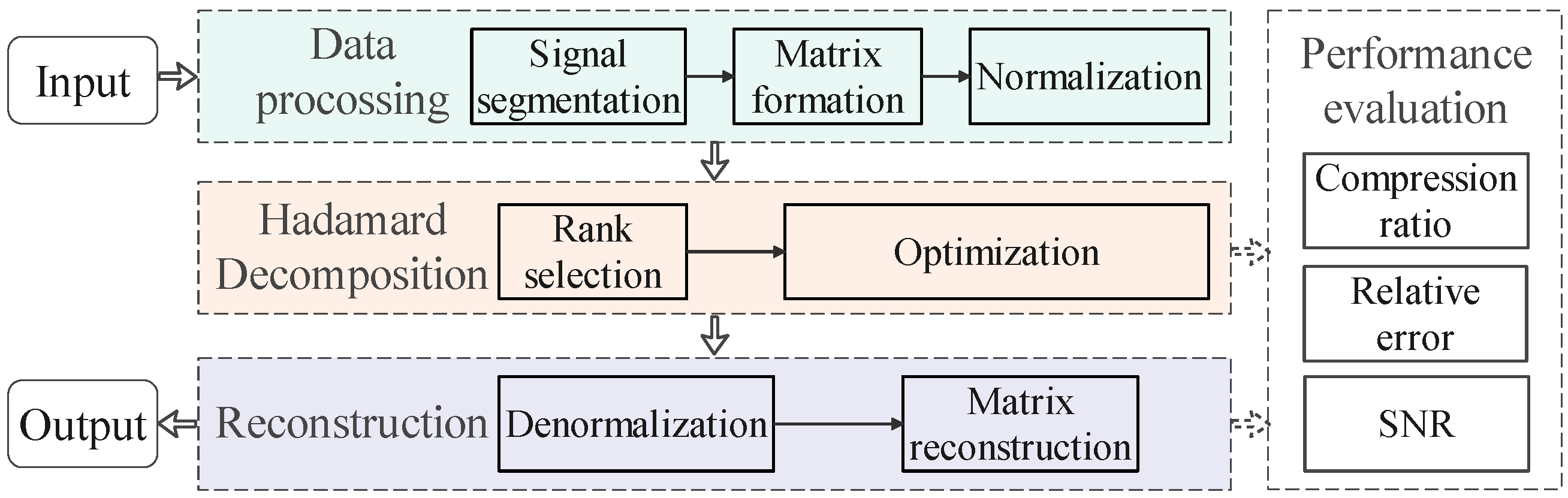
4. Data Compression Scheme for Power Quality Disturbance Analysis in Power Systems

In the context of increasingly complex power systems, efficient processing and analysis of power signal data have become crucial. This paper proposes a signal compression scheme based on Hadamard decomposition, aiming to achieve efficient compression and feature preservation. Figure 1 illustrates the process flow of the proposed scheme.

4.1. Data Preprocessing

The initial stage involves preprocessing the data for Hadamard decomposition:

• Signal Segmentation: During the collection process, divide the data into data segments of length N.
• Matrix Formation: Arrange each segment into an $N\times N$ matrix. For signals that do not perfectly fit this square matrix, zero-padding can be applied.
• Normalization: Scale the data to a range of [0, 1] to ensure consistent processing across different types of disturbances:

  $$x_{\mathrm{norm}}={\displaystyle \frac{x-x_{min}}{x_{max}-x_{min}}}$$

  (15)

  where x is the original value, and $x_{min}$ and $x_{max}$ are the minimum and maximum values in the segment, respectively.

4.2. Decomposition

Apply the Hadamard decomposition algorithm described in Section 3 to each preprocessed matrix. The key steps include:

• Rank Selection: Choose an appropriate rank r for the decomposition matrix. For signals with high complexity and rich information content, a larger r is typically needed to capture the essential features without a significant loss in accuracy. Conversely, for simpler signals or signals with less variation, a smaller r may suffice, offering a better compression ratio with minimal loss of relevant information.
  Additionally, the rank r should be chosen such that it strikes an optimal balance between the compression ratio (CR) and the relative reconstruction error (RE) as described in Section 4.4. A smaller rank reduces the storage requirements and computational cost, but this comes at the expense of reconstruction accuracy. Therefore, the rank r is selected by iterating through different values and evaluating the trade-offs using metrics such as RE and CR, ensuring that the rank provides sufficient accuracy while achieving the desired compression.
• Optimization: Use the gradient descent algorithm to find the optimal $U_1$, $V_1$, $U_2$, and $V_2$ matrices that minimize the reconstruction error.

4.3. Reconstruction

When the compressed data needs to be analyzed:

• Matrix Reconstruction: Compute the Hadamard product $\left(U_1{V}_1\right)\odot \left(U_2{V}_2\right)$ to obtain the approximated disturbance data matrix.
• Denormalization: Apply the inverse of the normalization step to recover the original scale of the data.

4.4. Performance Evaluation

To assess the effectiveness of the proposed scheme across different types of PQDs, we evaluate its performance using the following metrics:

• Relative error (RE), as defined in Equation (13), measures the reconstruction accuracy for each type of disturbance. A smaller RE indicates a more accurate decomposition, with RE = 0 representing a perfect reconstruction.
• Signal-to-noise ratio (SNR) quantifies the quality of the reconstructed signal compared to the original signal, and provides a logarithmic measure of the decomposition quality. A higher SNR indicates better decomposition quality, with each 3 dB increase corresponding to approximately halving the reconstruction error power. The formula for calculating SNR is as follows:

  $$\mathrm{SNR}=10lg\left({\displaystyle \frac{{\left|\right|M\left|\right|}_F^2}{\left|\right|M-\left(U_1{V}_1\right)\odot \left(U_2{V}_2\right){\left|\right|}_F^2}}\right)$$

  (16)
• Compression ratio (CR) determines the extent of data reduction achieved for each disturbance type:

  $$\mathrm{CR}={\displaystyle \frac{2r(n+m)}{nm}}$$

  (17)

  where n and m are the dimensions of the original matrix M, and r is the rank of the decomposition matrix. This ratio compares the number of elements in the decomposed matrices $U_1,V_1,U_2,V_2$ to the number of elements in the original matrix M. A lower CR indicates higher compression.

5. Simulation Studies

Power quality monitoring and analysis are crucial aspects in modern power systems, particularly given the increasing complexity introduced by renewable energy integration and power electronic devices. Among various power system measurements, PQD data are especially representative, as they capture both steady-state variations and transient events, making them an ideal candidate for validating compression methods. This section presents comprehensive validation studies of the proposed compression scheme through both simulated and field-collected PQD data. The simulated signals adopt voltage waveforms to emulate steady-state and transient events, while field experiments utilize current and voltage measurements from distribution networks. This dual-validation strategy demonstrates the scheme’s adaptability to two key power signal types with similar data modalities.

5.1. Simulation Model

PQDs are usually caused by faults, load changes, or the operation of nonlinear devices within a new-type power system. This paper focuses on several typical types of single and mixed PQDs, which are listed in

Table 1. Typical types of PQDs.

Disturbance	Code	Disturbance	Code
Sag	$D_1$	Oscillation + Interruption	$D_{13}$
Swell	$D_2$	Oscillation + Notch	$D_{14}$
Interruption	$D_3$	Sag + Interruption	$D_{15}$
Harmonics	$D_4$	Sag + Notch	$D_{16}$
Oscillation	$D_5$	Swell + Interruption	$D_{17}$
Notch	$D_6$	Swell + Notch	$D_{18}$
Harmonics + Sag	$D_7$	Harmonics + Sag + Interruption	$D_{19}$
Harmonics + Swell	$D_8$	Oscillation + Sag + Interruption	$D_{20}$
Harmonics + Interruption	$D_9$	Sag + Swell + Interruption	$D_{21}$
Harmonics + Notch	$D_{10}$	Harmonics + Sag + Swell + Interruption	$D_{22}$
Oscillation + Sag	$D_{11}$	Oscillation + Sag + Swell + Interruption	$D_{23}$
Oscillation + Swell	$D_{12}$	Harmonics + Oscillation + Sag + Swell	$D_{24}$

. An overview of the proposed simulation model is shown in Figure 2, which is established in PSCAD/EMTDC. Part 1 is used to simulate voltage sags, voltage swells, and momentary interruption caused by short-circuit faults. The duration time of these disturbances is adjusted by changing the duration time of short-circuit faults, and the types of disturbances are varied based on the specific short-circuit fault configuration. Part 2 focuses on flicker disturbances, which are caused by minor, periodic fluctuations in system frequency. Part 3 is a branch operating under normal conditions, where induction motors are connected in series with a step-down transformer, which may result in oscillation disturbances. Part 4 simulates harmonic disturbances, which are usually caused by converter stations in high-voltage transmission systems. The components and amplitudes of harmonics are varied by changing the types of rectifier bridges, their configuration, and the types of transformers used.

5.2. Simulation Results

One hundred sets of each type of disturbance are generated, with each set containing 16,384 consecutive sampling points and sampling frequency $f_s$ = 12.8 kHz. Each set is then rearranged into a 128 × 128 matrix for processing.

The performance metrics of the proposed scheme are averaged over the 100 sets for each disturbance type. The results shown in Figure 3 and

Table 2. Performance of the proposed scheme under different CRs based on simulated PQDs data.

PQDs	RE/p.u.			SNR/dB
	CR = 0.25	CR = 0.50	CR = 0.75	CR = 0.25	CR = 0.50	CR = 0.75
$D_1$	0.105 ± 0.054	0.061 ± 0.058	0.038 ± 0.025	32.86 ± 10.46	41.80 ± 12.10	47.68 ± 8.54
$D_2$	0.126±0.054	0.086 ± 0.070	0.058 ± 0.044	30.69 ± 9.81	37.72 ± 12.95	45.37 ± 11.93
$D_3$	0.094 ± 0.063	0.052 ± 0.043	0.042 ± 0.026	35.45 ± 12.07	44.50 ± 11.42	47.18 ± 8.19
$D_4$	0.021 ± 0.009	0.018 ± 0.008	0.019 ± 0.007	44.39 ± 3.59	45.95 ± 3.84	45.28 ± 3.50
$D_5$	0.116 ± 0.055	0.082 ± 0.070	0.058 ± 0.047	31.46 ± 9.42	38.22 ± 12.69	43.86 ± 11.20
$D_6$	0.106 ± 0.061	0.061 ± 0.059	0.050 ± 0.034	32.62 ± 9.17	39.23 ± 9.53	44.77 ± 8.42
$D_7$	0.086 ± 0.056	0.050 ± 0.049	0.030 ± 0.023	34.25 ± 8.12	40.16 ± 8.39	45.61 ± 5.87
$D_8$	0.140 ± 0.040	0.103 ± 0.057	0.071 ± 0.064	27.73 ± 4.03	32.54 ± 8.69	38.47 ± 11.02
$D_9$	0.079 ± 0.054	0.060 ± 0.055	0.022 ± 0.021	34.81 ± 7.64	38.36 ± 8.50	45.96 ± 5.25
$D_{10}$	0.028 ± 0.013	0.022 ± 0.012	0.021 ± 0.007	41.85 ± 3.77	44.08 ± 4.31	44.21 ± 3.10
$D_{11}$	0.094 ± 0.063	0.065 ± 0.064	0.051 ± 0.033	35.23 ± 11.42	40.51 ± 11.88	46.54 ± 9.68
$D_{12}$	0.138 ± 0.033	0.111 ± 0.053	0.092 ± 0.069	27.59 ± 3.33	31.98 ± 9.44	36.49 ± 12.40
$D_{13}$	0.096 ± 0.062	0.050 ± 0.037	0.041 ± 0.024	34.47 ± 10.63	45.41 ± 10.01	47.64 ± 7.34
$D_{14}$	0.114 ± 0.055	0.080 ± 0.066	0.047 ± 0.031	31.63 ± 9.40	38.03 ± 12.05	46.80 ± 9.51
$D_{15}$	0.071 ± 0.056	0.043 ± 0.029	0.014 ± 0.014	38.22 ± 11.50	46.70 ± 9.08	48.76 ± 4.66
$D_{16}$	0.076 ± 0.058	0.052 ± 0.041	0.035 ± 0.021	27.80 ± 11.78	44.08 ± 10.05	48.16 ± 7.34
$D_{17}$	0.105 ± 0.066	0.073 ± 0.066	0.051 ± 0.036	34.38 ± 12.08	39.58 ± 12.62	45.59 ± 9.81
$D_{18}$	0.130 ± 0.046	0.103 ± 0.061	0.086 ± 0.067	29.39 ± 7.53	33.77 ± 10.78	37.24 ± 12.48
$D_{19}$	0.092 ± 0.045	0.068 ± 0.060	0.049 ± 0.027	31.78 ± 8.93	34.36 ± 7.78	39.47 ± 8.03
$D_{20}$	0.097 ± 0.036	0.078 ± 0.075	0.058 ± 0.045	29.43 ± 6.98	33.01 ± 7.18	36.42 ± 10.11
$D_{21}$	0.093 ± 0.056	0.062 ± 0.021	0.048 ± 0.027	33.20 ± 10.85	35.74 ± 11.20	40.98 ± 9.63
$D_{22}$	0.115 ± 0.089	0.092 ± 0.067	0.071 ± 0.022	30.23 ± 6.59	31.81 ± 8.24	33.83 ± 8.36
$D_{23}$	0.116 ± 0.080	0.096 ± 0.068	0.074 ± 0.060	29.30 ± 12.08	31.71 ± 12.24	32.19 ± 10.63
$D_{24}$	0.130 ± 0.072	0.101 ± 0.041	0.096 ± 0.023	26.20 ± 9.69	28.93 ± 8.75	32.54 ± 10.08

indicate that the proposed scheme achieves high compression efficiency while maintaining satisfactory reconstruction quality across various types of PQDs. At CR = 0.50, the average relative error across all PQD types is approximately 0.070, i.e., 7%, indicating that 93% of the original signal information is preserved. When the CR increases to 0.75, the average RE decreases to about 0.050 (5%), demonstrating enhanced information preservation with minimal increase in storage requirements. Experimental results also demonstrate robust performance for complex disturbances involving three or more events. Even for the most challenging cases involving multiple disturbances $D_{19}$ to $D_{24}$, the RE remains below 0.10, ensuring that at least 90% of the original information is retained.

Additionally, as shown in Table 2, the RE and SNR for disturbances involving harmonics and oscillations exhibit lower SNR and higher RE compared to other types of disturbances. For instance, in the case of a mixed PQD involving three components, $D_{20}$ shows RE = 0.097 ± 0.036 and SNR = 30.23 ± 6.59 at CR = 0.25, with minimal SNR improvement to 36.42 ± 10.11 at CR = 0.75. Similarly, for a mixed PQD involving four components, $D_{24}$ achieves RE = 0.096 ± 0.023 and SNR = 32.54 ± 10.08 at CR = 0.75, reflecting the challenge of capturing non-stationary components within low-rank approximations.

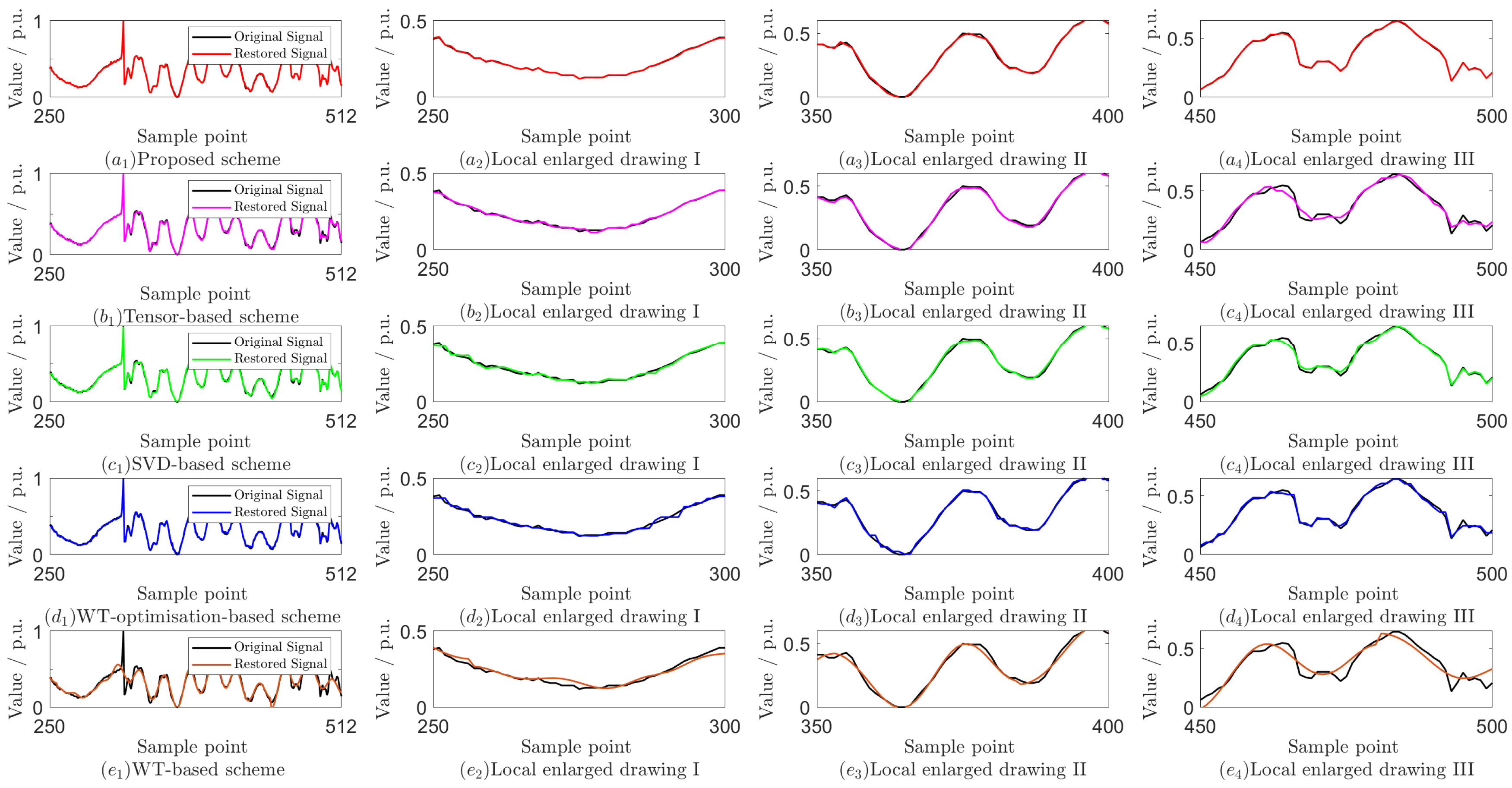
5.3. Field Data Test and Performance Comparison

Compared to simulation data, the waveform variations in field-collected data are more complex. In this paper, we utilize field data from a pilot distribution network in Fujian Province, China, where an instantaneous BC phase fault occurred outside the differential protection zone on the 10 kV side of the main transformer. The dataset includes six sets of three-phase current and voltage signals, each containing 512 sample points. Due to the complex network structure and various electrical equipments, there have been significant abnormal fluctuations in the current and voltage waveforms.

Taking the collected A-phase current signal as an example, Figure 4 shows the original signal with their restored signals using different compression methods. It can be seen that all methods have good reconstruction effects, but the proposed scheme can better reconstruct the abrupt parts in the signal. To futher evaluate the proposed scheme’s performance, we compare it with several advanced compression methods frequently employed in power systems. The results presented in

Table 3. Performance comparison with other advanced compression methods based on the field data.

Literature	Method	CR = 0.25		CR = 0.50		CR = 0.75
		RE/p.u.	SNR/dB	RE/p.u.	SNR/dB	RE/p.u.	SNR/dB
Ref. [15]	Tensor decomposition	0.073	33.43	0.024	43.75	0.008	55.00
Ref. [16]	SVD	0.062	26.13	0.013	39.95	0.004	51.36
Ref. [19]	Wavelet spectral quantization	0.047	28.31	0.007	45.86	0.002	60.41
Ref. [22]	Huffman coding &Run-length coding	0.097	31.34	0.021	45.10	0.010	53.22
Ref. [29]	WT &Particle Swarm Optimisation	0.099	28.22	0.026	40.01	0.011	56.89
Proposed scheme	Hadamard decomposition	0.023	34.37	0.005	49.21	0.003	68.24

indicate that the proposed scheme consistently yields lower RE and higher SNR across various REs, achieving a favorable balance between compression efficiency and reconstruction accuracy.

5.4. Discussion

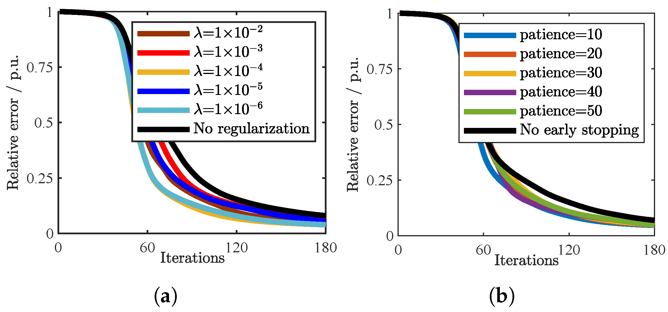
5.4.1. Sensitivity Analysis

To assess the robustness of the proposed method, we conducted a sensitivity analysis on data granularity, which is defined by varying matrix sizes through adjustments to the sampling frequency. As shown in

Table 4. Performance of the proposed scheme under different data granularities.

Sampling Frequency	Data Granularity	CR = 0.25 (RE/SNR)	CR = 0.50 (RE/SNR)	CR = 0.75 (RE/SNR)
0.8 kHz	32 × 32	0.090 ± 0.047/39.52 ± 7.33	0.052 ± 0.035/43.20 ± 8.26	0.027 ± 0.021/48.99 ± 7.73
3.2 kHz	64 × 64	0.095 ± 0.054/34.63 ± 9.75	0.062 ± 0.038/41.85 ± 9.53	0.039 ± 0.030/47.70 ± 8.51
12.8 kHz	128 × 128	0.099 ± 0.053/32.71 ± 8.79	0.070 ± 0.051/38.26 ± 9.75	0.051 ± 0.033/42.54 ± 8.63

, higher sampling frequencies correspond to finer granularity, but slightly degrade compression performance compared to coarser granularity. For instance, at CR = 0.75, the RE increases from 0.027 ± 0.021 (0.8 kHz, 32 × 32) to 0.051 ± 0.033 (12.8 kHz, 128 × 128), while the SNR decreases by approximately 6.45 dB. The robust performance across different granularity levels validates the method’s practical applicability in various data scenarios.

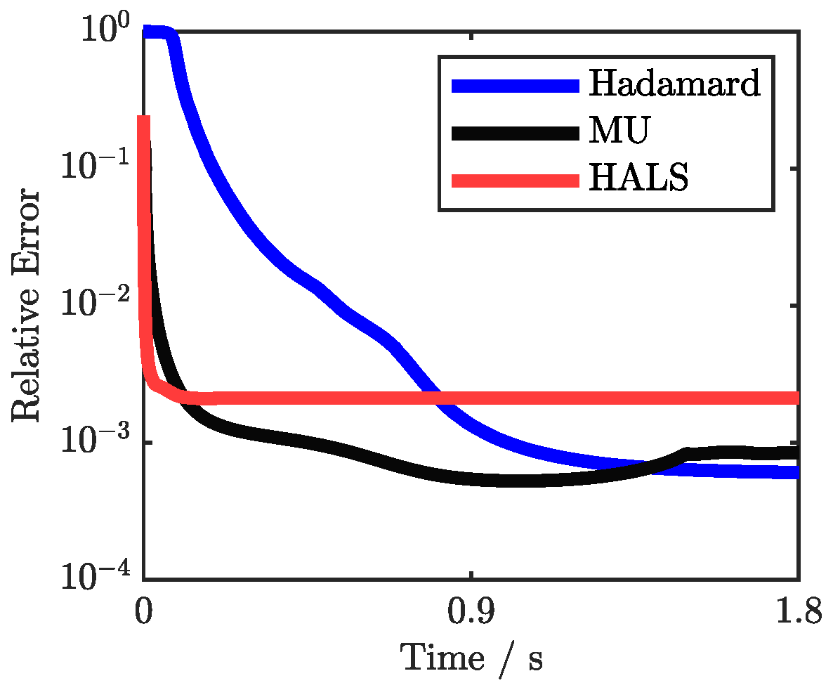
5.4.2. Convergence Performance Analysis

To investigate the impact of regularization parameters on the enhanced gradient descent algorithm, we compared our proposed method to the traditional gradient descent algorithm. Figure 5a illustrates the results based on experiments conducted using 1800 sets of PQD simulation data with patience = 50, and shows the relative error over 180 iterations for various regularization parameters, as well as a case with no regularization. It is evident that under the same number of iterations, the relative error with regularization is smaller than without regularization. Notably, the presence or absence of regularization had no significant impact on the running time, with all cases completing 180 iterations in approximately 60 ms.

Figure 5b further demonstrates the effectiveness of our early stopping mechanism, where different patience values are compared and $\lambda$ = 1 ×${10}^{-6}$. The results indicate that the early stopping mechanism helps achieve faster convergence by preventing unnecessary iterations while maintaining optimization stability.

Based on the convergence performance comparison with other optimization algorithms shown in Figure 6, while Multiplicative Updates (MU) and Hierarchical Alternating Least Squares (HALS) algorithms demonstrate superior overall convergence rates, the Hadamard decomposition exhibits unique convergence characteristics. The Hadamard decomposition maintains stable convergence behavior without oscillations, suggesting reliable performance for practical applications. This convergence pattern, combined with the algorithm’s structured nature and lower computational complexity, represents an effective balance between computational efficiency and optimization accuracy.

5.4.3. Frequency Domain Analysis

In new-type power systems, the widespread integration of power electronic devices, renewable energy sources, and non-linear loads introduces many harmonic components into the power grid. These harmonics are crucial indicators for system state assessment and power quality evaluation. Therefore, it is essential to evaluate the ability of the proposed scheme to preserve frequency domain information. Figure 7 presents a comparison of the frequency spectra between original and restored signals for $D_4$, $D_7$, and $D_8$, revealing that the proposed scheme effectively retains a substantial portion of the frequency domain information. The preservation of spectral content highlights its potential applicability in scenarios that require comprehensive analysis across both the time and frequency domains.

5.4.4. Packet Loss Analysis

In power system data transmission, packet loss during network communication may significantly impact the effectiveness of data compression schemes, potentially leading to degraded reconstruction quality and compromised system monitoring capabilities. To evaluate this impact, the packet loss effect on reconstruction performance is systematically analyzed across different CRs. In this study, packet loss is simulated by randomly setting elements in the decomposed matrices to zero, with the packet loss rate defined as the ratio of zeroed elements to the total number of matrix elements. Figure 8 illustrates the relationship between packet loss rate, CR, and reconstruction quality metrics (SNR and RE), revealing that performance degradation exhibits a non-linear relationship with both packet loss rate and CR. The results demonstrate the robustness of the proposed scheme under various network conditions.

6. Conclusions

This paper improves the traditional Hadamard decomposition by ensuring the uniqueness of decomposition results through theoretical constraints, and develops an enhanced gradient descent algorithm for optimizing the approximation of Hadamard decomposition. Based on these improvements, a novel Hadamard-decomposition-based data compression scheme for PQDs in new-type power systems is designed. By decomposing the PQD data matrix into the Hadamard product of two low-rank matrices, the proposed compression scheme achieves significant data reduction while preserving essential signal characteristics.

Comprehensive simulation studies demonstrate the effectiveness of the proposed scheme across various single and mixed PQDs. Furthermore, comparisons with other compression methods using field data reveal that our scheme offers a favorable balance between compression efficiency and reconstruction accuracy. The scheme also shows particular strength in preserving frequency domain information, making it suitable for power quality analysis applications where spectral characteristics are crucial.

Despite these achievements, certain limitations and challenges remain in the current framework. A primary limitation is that the Hadamard decomposition results lack clear physical interpretability, making it challenging to directly relate the decomposed matrices to specific data characteristics. Future work should focus on investigating the deeper mathematical implications of multiplicative relationships in Hadamard decomposition and exploring more optimization algorithms, potentially leading to more interpretable decomposition results while further enhancing the efficiency and robustness of the decomposition process.

References

1. He, S.; Zhang, Y.; Zhu, R.; Tian, W. Electric signature detection and analysis for power equipment failure monitoring in smart grid. IEEE Trans. Ind. Inform. 2020, 17, 3739–3750. [Google Scholar] [CrossRef]
2. Wang, W.; Chen, C.; Yao, W.; Sun, K.; Qiu, W.; Liu, Y. Synchrophasor data compression under disturbance conditions via cross-entropy-based singular value decomposition. IEEE Trans. Ind. Inform. 2020, 17, 2716–2726. [Google Scholar] [CrossRef]
3. Jian, J.; Zhao, J.; Ji, H.; Bai, L.; Xu, J.; Li, P.; Wu, J.; Wang, C. Supply restoration of data centers in flexible distribution networks with spatial-temporal regulation. IEEE Trans. Smart Grid 2023, 15, 340–354. [Google Scholar] [CrossRef]
4. Sun, J.; Chen, Q.; Xia, M. Data-driven detection and identification of line parameters with PMU and unsynchronized SCADA measurements in distribution grids. CSEE J. Power Energy Syst. 2022, 10, 261–271. [Google Scholar]
5. Senyuk, M.; Beryozkina, S.; Zicmane, I.; Safaraliev, M.; Klassen, V.; Kamalov, F. Bulk Low-Inertia Power Systems Adaptive Fault Type Classification Method Based on Machine Learning and Phasor Measurement Units Data. Mathematics 2025, 13, 316. [Google Scholar] [CrossRef]
6. Wang, X.; Liu, Y.; Tong, L. Adaptive subband compression for streaming of continuous point-on-wave and PMU data. IEEE Trans. Power Syst. 2021, 36, 5612–5621. [Google Scholar] [CrossRef]
7. Senyuk, M.; Safaraliev, M.; Pazderin, A.; Pichugova, O.; Zicmane, I.; Beryozkina, S. Methodology for Power Systems’ Emergency Control Based on Deep Learning and Synchronized Measurements. Mathematics 2023, 11, 4667. [Google Scholar] [CrossRef]
8. Pranitha, K.; Kavya, G. An efficient image compression architecture based on optimized 9/7 wavelet transform with hybrid post processing and entropy encoder module. Microprocess. Microsyst. 2023, 98, 104821. [Google Scholar] [CrossRef]
9. Liu, Q.; Huang, Z.; Chen, K.; Xiao, J. Efficient and Real-Time Compression Schemes of Multi-Dimensional Data from Ocean Buoys Using Golomb-Rice Coding. Mathematics 2025, 13, 366. [Google Scholar] [CrossRef]
10. Yan, L.; Han, J.; Xu, R.; Li, Z. Model-free lossless data compression for real-time low-latency transmission in smart grids. IEEE Trans. Smart Grid 2020, 12, 2601–2610. [Google Scholar] [CrossRef]
11. Chen, C.; Wang, W.; Yin, H.; Zhan, L.; Liu, Y. Real-time lossless compression for ultrahigh-density synchrophasor and point-on-wave data. IEEE Trans. Ind. Electron. 2021, 69, 2012–2021. [Google Scholar] [CrossRef]
12. Podgorelec, D.; Strnad, D.; Kolingerová, I.; Žalik, B. State-of-the-Art Trends in Data Compression: COMPROMISE Case Study. Entropy 2024, 26, 1032. [Google Scholar] [CrossRef] [PubMed]
13. Jeromel, A.; Žalik, B. An efficient lossy cartoon image compression method. Multimed. Tools Appl. 2020, 79, 433–451. [Google Scholar] [CrossRef]
14. Liu, T.; Wang, J.; Liu, Q.; Alibhai, S.; Lu, T.; He, X. High-ratio lossy compression: Exploring the autoencoder to compress scientific data. IEEE Trans. Big Data 2021, 9, 22–36. [Google Scholar] [CrossRef]
15. He, S.; Geng, X.; Tian, W.; Yao, W.; Dai, Y.; You, L. Online Compression of Multichannel Power Waveform Data in Distribution Grid with Novel Tensor Method. IEEE Trans. Instrum. Meas. 2024, 73, 6505011. [Google Scholar] [CrossRef]
16. Pourramezan, R.; Hassani, R.; Karimi, H.; Paolone, M.; Mahseredjian, J. A real-time synchrophasor data compression method using singular value decomposition. IEEE Trans. Smart Grid 2021, 13, 564–575. [Google Scholar] [CrossRef]
17. de Souza, J.C.S.; Assis, T.M.L.; Pal, B.C. Data compression in smart distribution systems via singular value decomposition. IEEE Trans. Smart Grid 2015, 8, 275–284. [Google Scholar] [CrossRef]
18. Hashemipour, N.; Aghaei, J.; Kavousi-Fard, A.; Niknam, T.; Salimi, L.; del Granado, P.C.; Shafie-Khah, M.; Wang, F.; Catalão, J.P. Optimal singular value decomposition based big data compression approach in smart grids. IEEE Trans. Ind. Appl. 2021, 57, 3296–3305. [Google Scholar] [CrossRef]
19. Nascimento, F.A.d.O.; Saraiva, R.G.; Cormane, J. Improved transient data compression algorithm based on wavelet spectral quantization models. IEEE Trans. Power Deliv. 2020, 35, 2222–2232. [Google Scholar] [CrossRef]
20. Yang, J.; Yu, H.; Li, P.; Ji, H.; Xi, W.; Wu, J.; Wang, C. Real-time D-PMU data compression for edge computing devices in digital distribution networks. IEEE Trans. Power Syst. 2023, 39, 5712–5725. [Google Scholar] [CrossRef]
21. Mishra, M.; Sen Gupta, G.; Gui, X. Investigation of energy cost of data compression algorithms in WSN for IoT applications. Sensors 2022, 22, 7685. [Google Scholar] [CrossRef] [PubMed]
22. Xiao, X.; Li, K.; Zhao, C. A Hybrid Compression Method for Compound Power Quality Disturbance Signals in Active Distribution Networks. J. Mod. Power Syst. Clean Energy 2023, 11, 1902–1911. [Google Scholar] [CrossRef]
23. Bello, I.A.; McCulloch, M.D.; Rogers, D.J. A linear regression data compression algorithm for an islanded DC microgrid. Sustain. Energy Grids Netw. 2022, 32, 2352–4677. [Google Scholar] [CrossRef]
24. Horn, R.A.; Yang, Z. Rank of a Hadamard product. Linear Algebra Its Appl. 2020, 591, 87–98. [Google Scholar] [CrossRef]
25. Wu, C.W. ProdSumNet: Reducing model parameters in deep neural networks via product-of-sums matrix decompositions. arXiv 2018, arXiv:1809.02209. [Google Scholar]
26. Yang, Z.; Stoica, P.; Tang, J. Source resolvability of spatial-smoothing-based subspace methods: A hadamard product perspective. IEEE Trans. Signal Process. 2019, 67, 2543–2553. [Google Scholar] [CrossRef]
27. Hyeon-Woo, N.; Ye-Bin, M.; Oh, T.H. Fedpara: Low-rank hadamard product for communication-efficient federated learning. arXiv 2021, arXiv:2108.06098. [Google Scholar]
28. Ciaperoni, M.; Gionis, A.; Mannila, H. The Hadamard decomposition problem. Data Min. Knowl. Discov. 2024, 38, 2306–2347. [Google Scholar] [CrossRef]
29. Karthika, S.; Rathika, P. An adaptive data compression technique based on optimal thresholding using multi-objective PSO algorithm for power system data. Appl. Soft Comput. 2024, 150, 111028. [Google Scholar] [CrossRef]
Figure 1. Flowchart of the proposed scheme.
Mathematics 13 00671 g001
Figure 2. Electrical diagram of the proposed simulation model.
Mathematics 13 00671 g002
Figure 3. Comparison between original signals and restored signals, where figure (af) correspond to D 1 to D 6 , respectively.
Mathematics 13 00671 g003
Figure 4. Original A-phase current signal with its restored signals [14,15,21,29].
Mathematics 13 00671 g004
Figure 5. Convergence performance of the proposed scheme with different parameters: (a) regularization parameter, (b) patience value.
Mathematics 13 00671 g005
Figure 6. Convergence performance comparison with the y-axis representing the logarithm of RE.
Mathematics 13 00671 g006
Figure 7. Frequency comparison between the original signal and the restored signal of D 4 , D 7 and D 8 .
Mathematics 13 00671 g007
Figure 8. Reconstruction performance under different packet loss rates.
Mathematics 13 00671 g008