
Modified Information Criterion for Testing Changes in the Inverse Gaussian Degradation Process


Abstract
1. Introduction
2. Changes in Inverse Gaussian Process
2.1. Inverse Gaussian Process
2.2. Inverse Gaussian Process with Change Points
3. Modified Information Criterion for Inverse Gaussian Process
3.1. Maximum Likelihood Estimators
3.2. Modified Information Criterion
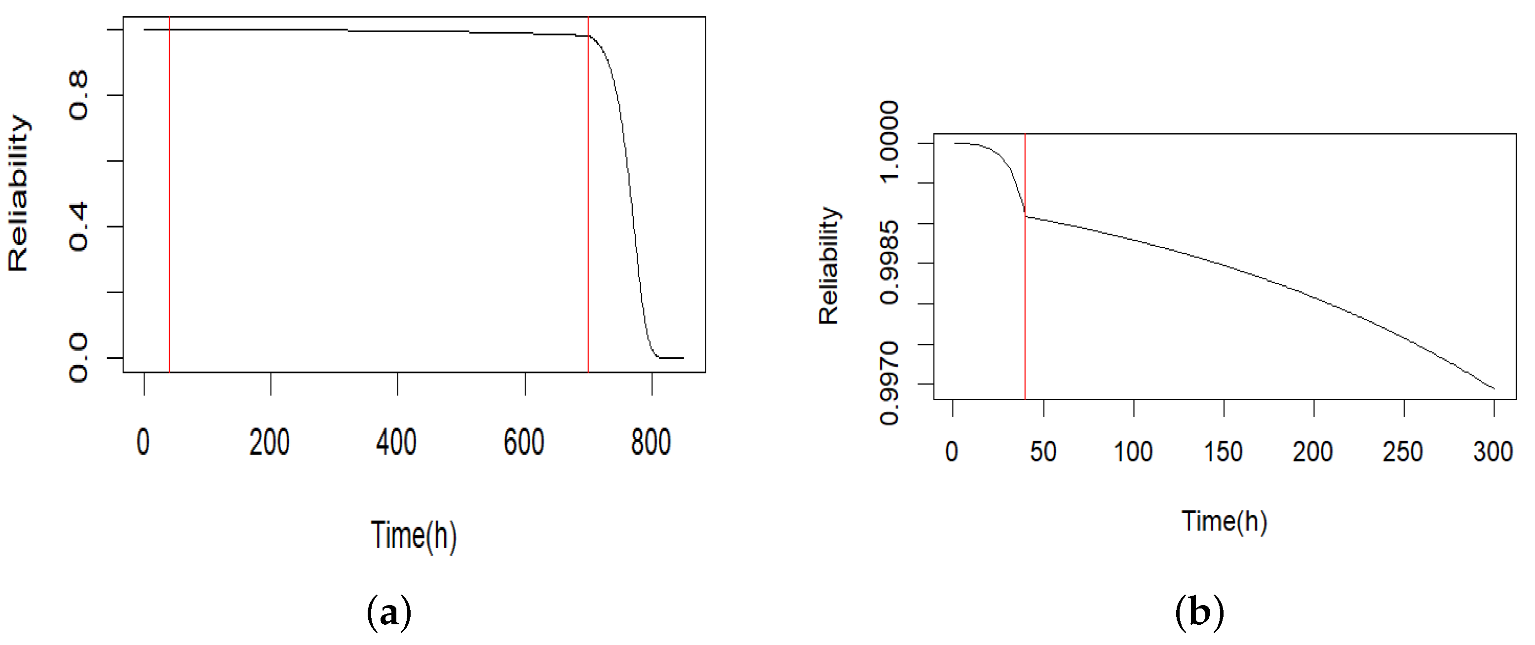
3.3. Reliability of the Change-Point Inverse Gaussian Process
4. Simulation
4.1. Power Comparison Between MIC and SIC
4.2. Consistency of Estimator Comparison
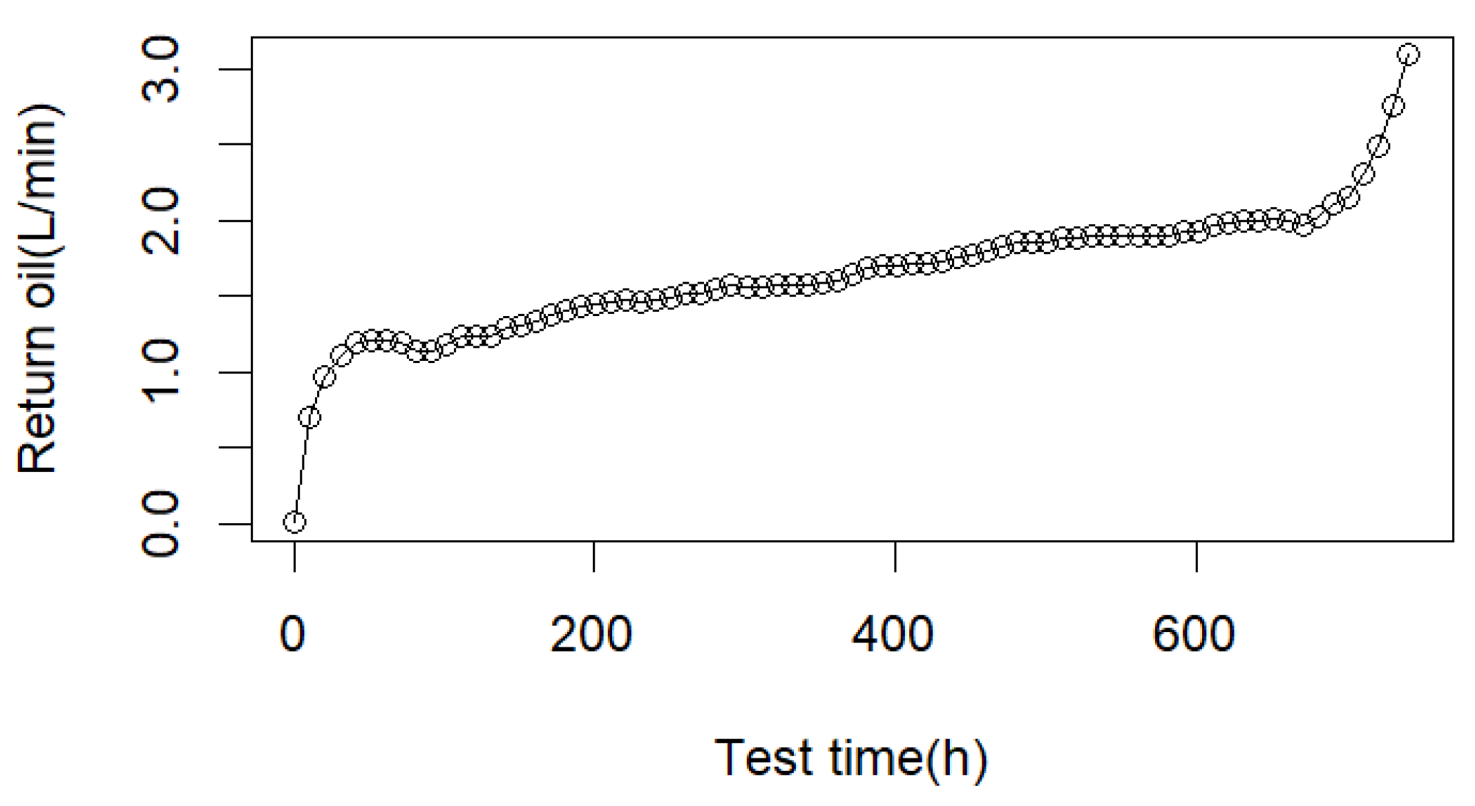
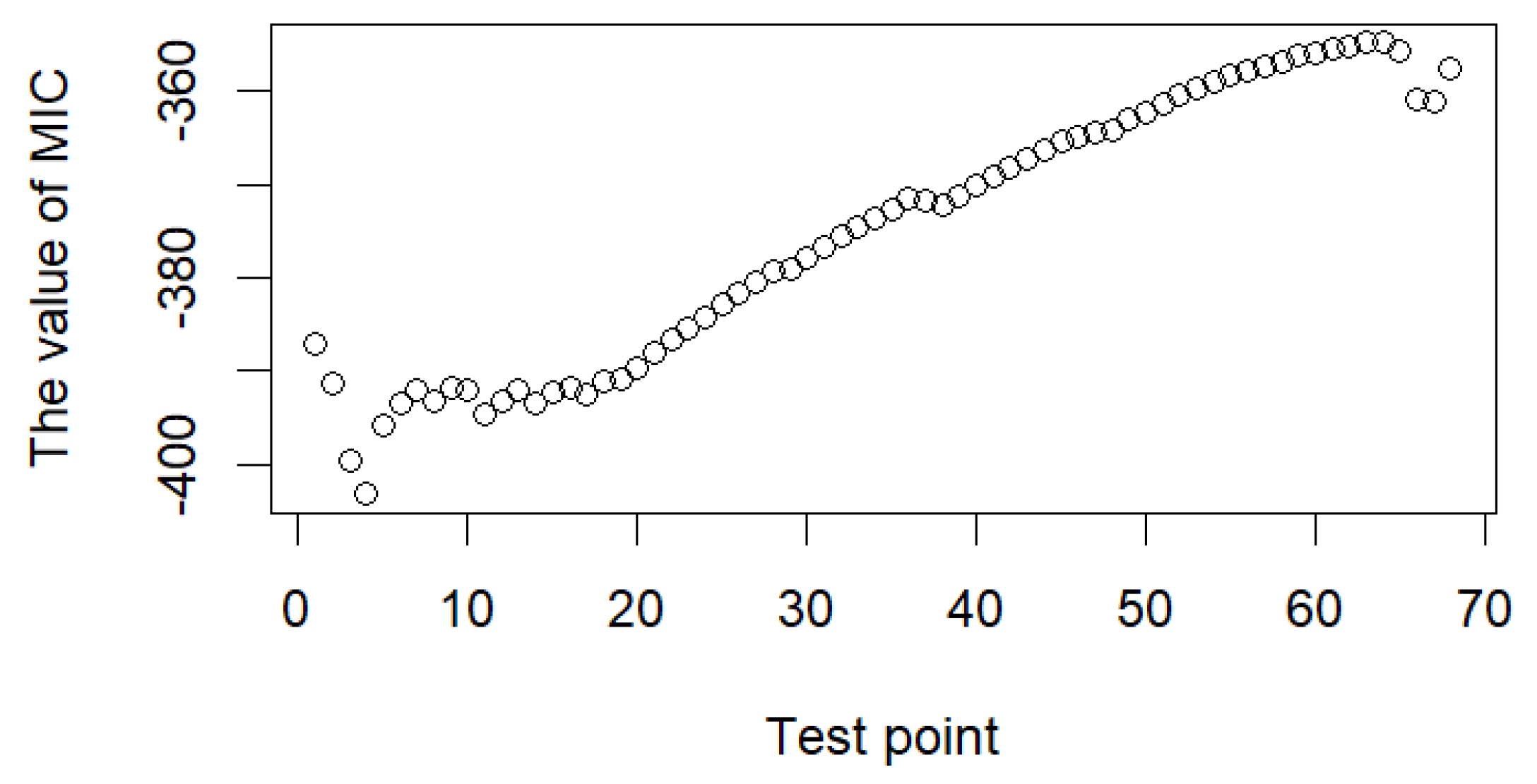
5. Application
6. Conclusions
Author Contributions
Funding
Data Availability Statement
Acknowledgments
Conflicts of Interest
Abbreviations
| PDP | plasma display panel |
| LCD | liquid crystal display |
| LED | light-emitting diode |
| IG | Inverse Gaussian |
| OLED | organic light-emitting diode |
| MOSFET | metal oxide semiconductor field-effect transistor |
| MCMC | Markov Chain Monte Carlo |
| CDF | cumulative distribution function |
| MLE | maximum likelihood estimation |
| AIC | Akaike Information Criterion |
| SIC | Schwartz Information Criterion |
| MIC | Modified Information Criterion |
Appendix A. Calculation Process of Equations (8)–(10)
Appendix B. Wald Conditions and Regular Conditions
Appendix B.1. Wald Conditions
Appendix B.2. Regular Conditions
Appendix C. Calculation of Equation (14)
References
- Hong, Y.; Duan, Y.; Meeker, W.Q.; Stanley, D.L.; Gu, X. Statistical Methods for Degradation Data with Dynamic Covariates Information and an Application to Outdoor Weathering Data. Technometrics 2015, 57, 180–193. [Google Scholar] [CrossRef]
- Ye, Z.; Xie, M. Stochastic Modelling and Analysis of Degradation for Highly Reliable Products. Appl. Stoch. Model. Bus. Ind. 2014, 31, 16–32. [Google Scholar] [CrossRef]
- Lu, C.J.; Meeker, W.O. Using Degradation Measures to Estimate a Time-to-Failure Distribution. Technometrics 1993, 35, 161–174. [Google Scholar] [CrossRef]
- Yu, H.-F. Designing an Accelerated Degradation Experiment with a Reciprocal Weibull Degradation Rate. J. Stat. Plan. Inference 2006, 136, 282–297. [Google Scholar] [CrossRef]
- Yuan, X.-X.; Pandey, M.D. A Nonlinear Mixed-Effects Model for Degradation Data Obtained from in-Service Inspections. Reliab. Eng. Syst. Saf. 2009, 94, 509–519. [Google Scholar] [CrossRef]
- Lu, L.; Wang, B.; Hong, Y.; Ye, Z. General Path Models for Degradation Data with Multiple Characteristics and Covariates. Technometrics 2020, 63, 354–369. [Google Scholar] [CrossRef]
- Ye, Z.-S.; Wang, Y.; Tsui, K.-L.; Pecht, M. Degradation Data Analysis Using Wiener Processes with Measurement Errors. IEEE Trans. Reliab. 2013, 62, 772–780. [Google Scholar] [CrossRef]
- Giorgio, M.; Mele, A.; Pulcini, G. A Perturbed Gamma Degradation Process with Degradation Dependent non-Gaussian Measurement Errors. Appl. Stoch. Model. Bus. Ind. 2018, 35, 198–210. [Google Scholar] [CrossRef]
- Fang, G.; Pan, R.; Wang, Y. Inverse Gaussian Processes with Correlated Random Effects for Multivariate Degradation Modeling. Eur. J. Oper. Res. 2022, 300, 1177–1193. [Google Scholar] [CrossRef]
- Liang, Y.; Yan, Z.; Sun, L. Reliability Analysis of Inverse Gaussian Processes with Two-Stage Degenerate Paths. Heliyon 2024, 10, e34625. [Google Scholar] [CrossRef]
- Wang, R.; Zhu, M.; Zhang, X.; Pham, H. Lithium-Ion Battery Remaining Useful Life Prediction Using a Two-Phase Degradation Model with a Dynamic Change Point. J. Energy Storage 2023, 59, 106457. [Google Scholar] [CrossRef]
- Wang, H.; Liao, H.; Ma, X. Stochastic Multi-Phase Modeling and Health Assessment for Systems Based on Degradation Branching Processes. Reliab. Eng. Syst. Saf. 2022, 222, 108412. [Google Scholar] [CrossRef]
- Sheng, Z.; Hu, Q.; Liu, J.; Yu, D. Residual Life Prediction for Complex Systems with Multi-Phase Degradation by ARMA-Filtered Hidden Markov Model. Qual. Technol. Quant. Manag. 2017, 16, 19–35. [Google Scholar] [CrossRef]
- Liu, K.; Zou, T.; Xin, M.; Lv, C. RUL Prediction Based on Two-phase Wiener Process. Qual. Reliab. Eng. Int. 2022, 38, 3829–3843. [Google Scholar] [CrossRef]
- Li, L.; Yu, T.; Shang, B.; Song, B.; Chen, Y. Reliability Modeling of Competing Failure Processes with Multi-stage Degradation. Qual. Reliab. Eng. Int. 2023, 39, 1494–1517. [Google Scholar] [CrossRef]
- Bae, S.J.; Yuan, T.; Ning, S.; Kuo, W. A Bayesian Approach to Modeling Two-Phase Degradation Using Change-Point Regression. Reliab. Eng. Syst. Saf. 2015, 134, 66–74. [Google Scholar] [CrossRef]
- Bae, S.J.; Yuan, T.; Kim, S. Bayesian Degradation Modeling for Reliability Prediction of Organic Light-Emitting Diodes. J. Comput. Sci. 2016, 17, 117–125. [Google Scholar] [CrossRef]
- Wang, P.; Tang, Y.; Joo Bae, S.; He, Y. Bayesian Analysis of Two-Phase Degradation Data Based on Change-Point Wiener Process. Reliab. Eng. Syst. Saf. 2018, 170, 244–256. [Google Scholar] [CrossRef]
- Wang, P.; Tang, Y.; Bae, S.J.; Xu, A. Bayesian Approach for Two-Phase Degradation Data Based on Change-Point Wiener Process with Measurement Errors. IEEE Trans. Reliab. 2018, 67, 688–700. [Google Scholar] [CrossRef]
- Wang, P.; Tang, Y.; Cheng, G. Degradation Data Analysis Based on Change-Point Gamma Process: A Bayesian Perspective. Chin. J. Appl. Probab. Stat. 2022, 38, 674–692. [Google Scholar]
- Zhuang, L.; Xu, A.; Wang, Y.; Tang, Y. Remaining Useful Life Prediction for Two-Phase Degradation Model Based on Reparameterized Inverse Gaussian Process. Eur. J. Oper. Res. 2024, 319, 877–890. [Google Scholar] [CrossRef]
- Bae, S.J.; Kvam, P.H. A Change-Point Analysis for Modeling Incomplete Burn-in for Light Displays. IIE Trans. 2006, 38, 489–498. [Google Scholar] [CrossRef]
- Kong, D.; Balakrishnan, N.; Cui, L. Two-Phase Degradation Process Model with Abrupt Jump at Change Point Governed by Wiener Process. IEEE Trans. Reliab. 2017, 66, 1345–1360. [Google Scholar] [CrossRef]
- Ling, M.H.; Ng, H.K.T.; Tsui, K.L. Bayesian and Likelihood Inferences on Remaining Useful Life in Two-Phase Degradation Models under Gamma Process. Reliab. Eng. Syst. Saf. 2019, 184, 77–85. [Google Scholar] [CrossRef]
- Vostrikova, L.J. Some Results about Multidimensional Branching Processes with Random Environments. Ann. Probab. 1974, 2, 441–455. [Google Scholar]
- Akaike, H.; Petrov, B.N.; Czaki, F. Information Theory and an Extension of the Maximum Likelihood Principle. In Second International Symposium on Information Theory; Springer: New York, NY, USA, 1973; pp. 267–281. [Google Scholar]
- Schwarz, G. Estimating the Dimension of a Model. Ann. Stat. 1978, 6, 31–38. [Google Scholar] [CrossRef]
- Chen, J.; Gupta, A.; Pan, J. Information Criterion and Change Point Problem for Regular Models. Sankhyā Indian J. Stat. 2006, 68, 252–282. [Google Scholar]
- Inclán, C.; Tiao, G.C. Use of sums of squares for retrospective detection of changes of variance. J. Am. Stat. Assoc. 1994, 89, 913–923. [Google Scholar]
- Gombay, E.; Horváth, L. An application of U-statistics to change-point analysis. Acta Sci. Math. 1995, 60, 345–357. [Google Scholar]
- Basalamah, D.; Said, K.K.; Ning, W.; Tian, Y. Modified information criterion for linear regression change-point model with its applications. Commun. Stat.-Simul. Comput. 2019, 50, 180–197. [Google Scholar] [CrossRef]
- Said, K.K.; Ning, W.; Tian, Y. Detecting changes in linear regression models with skew normal errors. Random Oper. Stoch. Equ. 2018, 26, 1–10. [Google Scholar] [CrossRef]
- Alghamdi, A.; Ning, W.; Gupta, A. An Information Approach for the Change Point Problem of the Rayleigh Lomax Distribution. Int. J. Intell. Technol. Appl. Stat. 2018, 11, 233–254. [Google Scholar]
- Said, K.K.; Ning, W.; Tian, Y. Modified information criterion for testing changes in skew normal model. Braz. J. Probab. Stat. 2019, 33, 280–300. [Google Scholar] [CrossRef]
- Ma, Z.; Wang, S.; Liao, H.; Zhang, C. Engineering-driven Performance Degradation Analysis of Hydraulic Piston Pump Based on the Inverse Gaussian Process. Qual. Reliab. Eng. Int. 2019, 35, 2278–2296. [Google Scholar] [CrossRef]
- Liao, G.; Yin, H.; Chen, M.; Lin, Z. Remaining useful life prediction for multi-phase deteriorating process based on Wiener process. Reliab. Eng. Syst. Saf. 2021, 207, 107361. [Google Scholar] [CrossRef]


| (1.5,3) | (1,2) | (1.5,2) | (1,1.5) | ||||||
|---|---|---|---|---|---|---|---|---|---|
| MIC | SIC | MIC | SIC | MIC | SIC | MIC | SIC | ||
| 30 | 7 | 0.817 | 0.651 | 0.256 | 0.124 | 0.569 | 0.382 | 0.169 | 0.077 |
| 15 | 0.964 | 0.845 | 0.502 | 0.261 | 0.87 | 0.666 | 0.321 | 0.13 | |
| 22 | 0.854 | 0.669 | 0.289 | 0.152 | 0.721 | 0.537 | 0.249 | 0.124 | |
| 60 | 15 | 1.000 | 0.998 | 0.772 | 0.652 | 0.993 | 0.968 | 0.593 | 0.425 |
| 30 | 1.000 | 0.999 | 0.952 | 0.852 | 1.000 | 0.999 | 0.863 | 0.717 | |
| 45 | 0.999 | 0.997 | 0.794 | 0.648 | 0.998 | 0.989 | 0.661 | 0.518 | |
| 90 | 22 | 1.000 | 1.000 | 0.968 | 0.949 | 1.000 | 0.999 | 0.871 | 0.815 |
| 45 | 1.000 | 1.000 | 0.999 | 0.986 | 1.000 | 1.000 | 0.985 | 0.963 | |
| 67 | 1.000 | 1.000 | 0.973 | 0.956 | 1.000 | 1.000 | 0.916 | 0.875 | |
| 120 | 30 | 1.000 | 1.000 | 0.999 | 0.996 | 1.000 | 1.000 | 0.984 | 0.969 |
| 60 | 1.000 | 1.000 | 1.000 | 0.999 | 1.000 | 1.000 | 0.998 | 0.994 | |
| 90 | 1.000 | 1.000 | 0.999 | 0.997 | 1.000 | 1.000 | 0.989 | 0.975 | |
| (1.5,3) | (1,2) | (1.5,2) | (1,1.5) | ||||||
|---|---|---|---|---|---|---|---|---|---|
| MIC | SIC | MIC | SIC | MIC | SIC | MIC | SIC | ||
| 30 | 7 | 0.952 | 0.936 | 0.527 | 0.461 | 0.837 | 0.786 | 0.369 | 0.315 |
| 15 | 0.995 | 0.988 | 0.736 | 0.617 | 0.972 | 0.937 | 0.616 | 0.523 | |
| 22 | 0.954 | 0.937 | 0.557 | 0.492 | 0.923 | 0.882 | 0.46 | 0.398 | |
| 60 | 15 | 1.000 | 1.000 | 0.934 | 0.909 | 0.998 | 0.992 | 0.807 | 0.769 |
| 30 | 1.000 | 1.000 | 0.989 | 0.969 | 1.000 | 1.000 | 0.952 | 0.914 | |
| 45 | 1.000 | 1.000 | 0.918 | 0.891 | 0.998 | 0.994 | 0.839 | 0.793 | |
| 90 | 22 | 1.000 | 1.000 | 0.997 | 0.986 | 1.000 | 1.000 | 0.973 | 0.937 |
| 45 | 1.000 | 1.000 | 0.999 | 0.995 | 1.000 | 1.000 | 0.998 | 0.994 | |
| 67 | 1.000 | 1.000 | 0.997 | 0.989 | 1.000 | 1.000 | 0.972 | 0.946 | |
| 120 | 30 | 1.000 | 1.000 | 1.000 | 0.998 | 1.000 | 1.000 | 1.000 | 0.998 |
| 60 | 1.000 | 1.000 | 1.000 | 1.000 | 1.000 | 1.000 | 1.000 | 1.000 | |
| 90 | 1.000 | 1.000 | 0.999 | 0.997 | 1.000 | 1.000 | 0.998 | 0.996 | |
| (1.5,3) | (1,2) | (1.5,2) | (1,1.5) | ||||||
|---|---|---|---|---|---|---|---|---|---|
| MIC | SIC | MIC | SIC | MIC | SIC | MIC | SIC | ||
| 30 | 7 | 0.983 | 0.979 | 0.631 | 0.611 | 0.914 | 0.901 | 0.537 | 0.514 |
| 15 | 0.998 | 0.997 | 0.824 | 0.768 | 0.99 | 0.983 | 0.755 | 0.693 | |
| 22 | 0.987 | 0.983 | 0.685 | 0.648 | 0.965 | 0.952 | 0.618 | 0.597 | |
| 60 | 15 | 1.000 | 1.000 | 0.967 | 0.949 | 1.000 | 0.998 | 0.912 | 0.863 |
| 30 | 1.000 | 1.000 | 0.998 | 0.988 | 1.000 | 0.999 | 0.986 | 0.958 | |
| 45 | 1.000 | 1.000 | 0.961 | 0.932 | 1.000 | 0.997 | 0.926 | 0.894 | |
| 90 | 22 | 1.000 | 1.000 | 0.998 | 0.994 | 1.000 | 1.000 | 0.991 | 0.983 |
| 45 | 1.000 | 1.000 | 1.000 | 1.000 | 1.000 | 1.000 | 0.998 | 0.993 | |
| 67 | 1.000 | 1.000 | 0.998 | 0.995 | 1.000 | 1.000 | 0.993 | 0.989 | |
| 120 | 30 | 1.000 | 1.000 | 1.000 | 1.000 | 1.000 | 1.000 | 1.000 | 0.997 |
| 60 | 1.000 | 1.000 | 1.000 | 1.000 | 1.000 | 1.000 | 1.000 | 1.000 | |
| 90 | 1.000 | 1.000 | 1.000 | 1.000 | 1.000 | 1.000 | 0.999 | 0.996 | |
| MIC | SIC | MIC | SIC | MIC | SIC | MIC | SIC | ||
|---|---|---|---|---|---|---|---|---|---|
| 30 | 7 | 0.393 | 0.387 | 0.656 | 0.609 | 0.771 | 0.733 | 0.836 | 0.819 |
| 15 | 0.412 | 0.410 | 0.667 | 0.661 | 0.782 | 0.757 | 0.844 | 0.821 | |
| 22 | 0.408 | 0.393 | 0.653 | 0.610 | 0.754 | 0.725 | 0.813 | 0.797 | |
| 60 | 15 | 0.419 | 0.412 | 0.660 | 0.657 | 0.792 | 0.781 | 0.850 | 0.847 |
| 30 | 0.443 | 0.432 | 0.690 | 0.675 | 0.797 | 0.798 | 0.862 | 0.859 | |
| 45 | 0.421 | 0.420 | 0.661 | 0.658 | 0.773 | 0.755 | 0.837 | 0.832 | |
| 90 | 22 | 0.428 | 0.415 | 0.678 | 0.669 | 0.791 | 0.781 | 0.860 | 0.849 |
| 45 | 0.463 | 0.449 | 0.710 | 0.695 | 0.818 | 0.818 | 0.882 | 0.880 | |
| 67 | 0.449 | 0.447 | 0.696 | 0.674 | 0.806 | 0.801 | 0.879 | 0.872 | |
| 120 | 30 | 0.447 | 0.443 | 0.679 | 0.693 | 0.810 | 0.806 | 0.884 | 0.866 |
| 60 | 0.452 | 0.450 | 0.727 | 0.701 | 0.835 | 0.816 | 0.886 | 0.878 | |
| 90 | 0.451 | 0.445 | 0.718 | 0.683 | 0.830 | 0.809 | 0.881 | 0.875 | |
Disclaimer/Publisher’s Note: The statements, opinions and data contained in all publications are solely those of the individual author(s) and contributor(s) and not of MDPI and/or the editor(s). MDPI and/or the editor(s) disclaim responsibility for any injury to people or property resulting from any ideas, methods, instructions or products referred to in the content. |
© 2025 by the authors. Licensee MDPI, Basel, Switzerland. This article is an open access article distributed under the terms and conditions of the Creative Commons Attribution (CC BY) license (https://creativecommons.org/licenses/by/4.0/).
Share and Cite
Qiao, J.; Cai, X.; Zhang, M. Modified Information Criterion for Testing Changes in the Inverse Gaussian Degradation Process. Mathematics 2025, 13, 663. https://doi.org/10.3390/math13040663
Qiao J, Cai X, Zhang M. Modified Information Criterion for Testing Changes in the Inverse Gaussian Degradation Process. Mathematics. 2025; 13(4):663. https://doi.org/10.3390/math13040663
Chicago/Turabian StyleQiao, Jiahua, Xia Cai, and Meiqi Zhang. 2025. "Modified Information Criterion for Testing Changes in the Inverse Gaussian Degradation Process" Mathematics 13, no. 4: 663. https://doi.org/10.3390/math13040663
APA StyleQiao, J., Cai, X., & Zhang, M. (2025). Modified Information Criterion for Testing Changes in the Inverse Gaussian Degradation Process. Mathematics, 13(4), 663. https://doi.org/10.3390/math13040663