The General Solution to a System of Tensor Equations over the Split Quaternion Algebra with Applications

Abstract

This paper presents a systematic investigation into the solvability and the general solution of a tensor equation system within the split quaternion algebra framework. As an extension of classical quaternions with distinctive pseudo-Euclidean properties, split quaternions offer unique advantages in multidimensional signal processing applications. We establish rigorous necessary and sufficient conditions for the existence of solutions to the proposed tensor equation system, accompanied by explicit formulations for general solutions when solvability criteria are satisfied. The theoretical framework is further strengthened by the development of computational algorithms and numerical validations through concrete examples. Notably, we demonstrate the practical implementation of our theoretical findings through encryption/decryption algorithms for color video data.

1. Introduction

In 1843, William Rowan Hamilton introduced the concept of real quaternions [1] defined by

$$\mathbb{H}=\{q=q_0+q_{1}i+q_{2}j+q_{3}k:i^2=j^2=k^2=-1,ijk=-1,q_0,q_1,q_2,q_3\in \mathbb{R}\},$$

where $\mathbb{H}$ and $\mathbb{R}$, respectively, denote the set of real quaternions and the set of real numbers. Quaternions have been utilized in numerous areas, including the analysis of quaternion random signals [2], color image processing [3] and face recognition [4]. As the theory of quaternions evolved, James Cockle introduced the concept of split quaternions [5] in 1849:

$${\mathbb{Q}}_S=\{q=q_0+q_{1}i+q_{2}j+q_{3}k:q_0,q_1,q_2,q_3\in \mathbb{R}\},$$

where the imaginary identities $i,j,k$ satisfied

$$i^2=-1,j^2=k^2=1,ijk=1,$$

$$ij=-ji=k,jk=-kj=-i,ki=-ik=j.$$

Split quaternions have diverse applications across various fields. In physics, they are used to model spacetime symmetries and rotations in relativity [6]. In computer graphics, split quaternions assist in efficiently handling 3D rotations and transformations [7]. Split quaternions also have applications in control theory, signal processing, and robotics, where they help in representing and solving complex spatial relationships and transformations [8].

Tensors, as mathematical constructs that generalize scalars, vectors, and matrices to higher dimensions, are extensively applied across a wide range of scientific and engineering domains due to their capability to manage complex data structures. In computer vision and image processing, tensors are used to represent multidimensional image data, with convolution operations in neural networks being performed as tensor operations [9]. In physics, tensors are fundamental in general relativity for describing spacetime geometry [10] and in electromagnetism for unifying electric and magnetic fields [11]. In machine learning, tensors are core data structures in frameworks like TensorFlow and PyTorch, playing a crucial role in optimization and model training [12,13]. They are also essential in data analysis for dimensionality reduction and feature extraction, particularly within recommendation systems [14]. The multidimensional nature of tensors makes them powerful tools for handling complex data, and their significance continues to grow with advancements in computational power and algorithms.

$\mathcal{A}=\left(a_{i_1\cdots i_N}\right)(1\le i_j\le I_j,j=1,\dots ,N)$ presents an N-dimensional tensor, which is a natural extension of the matrix. For $N=1$, $\mathcal{A}$ is a vector. For $N=2$, $\mathcal{A}$ is a matrix. In recent decades, numerous researchers have made significant contributions to the study of tensors and quaternions. For example, Qi et al. [15,16,17,18,19] researched the spectral theory of tensor and tensor eigenvalues. Zhang et al. [20,21] investigated some terative solutions of generalized Sylvester quaternion tensor equations. Gao et al. [22] established the necessary and sufficient conditions for the existence of (anti-)$\eta$-Hermitian solutions to a system of matrix equations over split quaternion algebra. Xie et al. [23] proposed the BiCG algorithm for solving the minimal Frobenius norm solution of generalized Sylvester tensor equation over the quaternions. Yang et al. [24] researched a system of tensor equations over the dual split quaternion algebra with an application.

To the best of our knowledge, research on systems of tensor equations over split quaternions remains relatively scarce in the current literature. Building upon the aforementioned studies and leveraging the existing applications of tensor equation systems within split quaternion algebra, this paper aims to systematically investigate the solvability conditions and derive the general solution for the following system of split quaternion tensor equations

$$\left\{\begin{array}{c}{\mathcal{A}}_1{\ast }_N{\mathcal{X}}_1={\mathcal{P}}_1,\hfill \\ {\mathcal{X}}_1{\ast }_N{\mathcal{B}}_1={\mathcal{Q}}_1,\hfill \\ {\mathcal{A}}_2{\ast }_N{\mathcal{X}}_2={\mathcal{P}}_2,\hfill \\ {\mathcal{X}}_2{\ast }_N{\mathcal{B}}_2={\mathcal{Q}}_2,\hfill \\ \cdots \hfill \\ {\mathcal{A}}_n{\ast }_N{\mathcal{X}}_n={\mathcal{P}}_n,\hfill \\ {\mathcal{X}}_n{\ast }_N{\mathcal{B}}_n={\mathcal{Q}}_n,\hfill \\ {\displaystyle \sum _{t=1}^n}{\mathcal{E}}_t{\ast }_N{\mathcal{X}}_t{\ast }_N{\mathcal{F}}_t=\mathcal{H},\hfill \end{array}\right.$$

(1)

where ${\mathcal{A}}_t,{\mathcal{P}}_t,{\mathcal{B}}_t,{\mathcal{Q}}_t,{\mathcal{E}}_t,{\mathcal{F}}_t(t=1,\dots ,n)$ and $\mathcal{H}$ are given quaternion tensors and ${\mathcal{X}}_t(t=1,\dots ,n)$ are unknown split quaternion tensors.

Significantly, this study marks the first successful resolution of complex multilinear tensor equation systems over split quaternion algebra, representing a substantial advancement in the field. Moreover, our research can provide an application of split quaternion tensor equations in practical cryptographic implementations.

This paper is organized as follows: In Section 2, some basic theories and relevant properties of quaternion tensors are reviewed. In Section 3, we derive some practical necessary and sufficient conditions for the existence of the general solution to system (1) over ${\mathbb{Q}}_S$. Furthermore, the formula of the general solution to system (1) is also given when it is solvable. Especially, the unique solution is given when the uniqueness condition is satisfied. In Section 4, two algorithms and one numerical example are given in order to illustrate our results. In Section 5, we provide four algorithms and two examples for color video encryption and decryption. In Section 6, we present a conclusion to summarize this paper.

In subsequent sections, the symbols ${\mathbb{R}}^{m\times n}$, ${\mathbb{C}}^{m\times n}$, ${\mathbb{Q}}_S^n$, and ${\mathbb{Q}}_S^{m\times n}$ are used to represent the set of all $m\times n$ real matrices, all $m\times n$ complex matrices, all n dimensional split quaternion column vectors, and all $m\times n$ split quaternion matrices. The symbol $r\left(A\right)$ denotes the rank of the matrix A. I denotes the identity matrix and O the zero matrix with an appropriate size. $\overline{A},A^T,A^{\ast },A^{†}$ denote the conjugate, the transpose, the conjugate transpose, and the Moore–Penrose inverse of the matrix A, respectively. Let ${\mathbb{R}}^{I_1\times \cdots \times I_N\times J_1\times \cdots \times J_N},{\mathbb{C}}^{I_1\times \cdots \times I_N\times J_1\times \cdots \times J_N},$ and ${\mathbb{Q}}_S^{I_1\times \cdots \times I_N\times J_1\times \cdots \times J_N}$ represent the set of all corresponding dimensional real tensors, complex tensors, and split quaternion tensors, respectively.

2. Preliminaries

This section primarily introduces split quaternion tensors, the Einstein product of split quaternion tensors, the complex representation and related properties of split quaternion matrices, and so on. These concepts lay the groundwork for deriving the main conclusions presented in the subsequent sections.

Definition 1 

([25]). For two split quaternion tensors $\mathcal{A}=\left(a_{i_1\cdots i_N{j}_1\cdots j_L}\right)\in {\mathbb{Q}}_S^{I_1\times \cdots \times I_N\times J_1\times \cdots \times J_L}$ and $\mathcal{B}=\left(b_{j_1\cdots j_L{k}_1\cdots k_M}\right)\in {\mathbb{Q}}_S^{J_1\times \cdots \times J_L\times K_1\times \cdots \times K_M}$, the Einstein product of $\mathcal{A}$ and $\mathcal{B}$ is defined by the operation ${\ast }_L$ via

$${\left(\mathcal{A}{\ast }_L\mathcal{B}\right)}_{i_1\cdots i_N{k}_1\cdots k_M}=\sum _{j_1\cdots j_L}{a}_{i_1\cdots i_N{j}_1\cdots j_L}{b}_{j_1\cdots j_L{k}_1\cdots k_M},$$

where $\mathcal{A}{\ast }_L\mathcal{B}\in {\mathbb{Q}}_S^{I_1\times \cdots \times I_N\times K_1\times \cdots \times K_M}$.

The Einstein product of tensors is closely related to matrix multiplication. We introduce a mapping that establishes an isomorphic relationship between tensors with respect to the Einstein product and matrices with respect to the general matrix product.

Definition 2 

([26]). There exists an isomorphic mapping f from ${\mathbb{Q}}_S^{I_1\times \cdots \times I_N\times J_1\times \cdots \times J_N}$ to ${\mathbb{Q}}_S^{I\times J}$ denoted as

$$\begin{array}{ccc}\hfill f:{\mathbb{Q}}_S^{I_1\times \cdots \times I_N\times J_1\times \cdots \times J_N}& \to & {\mathbb{Q}}_S^{I\times J}\hfill \\ \hfill a_{i_1\cdots i_N{j}_1\cdots j_N}& \mapsto & a_{[i_N+{\sum }_{K=1}^{N-1}(i_K-1){\prod }_{S=K+1}^N{I}_S][j_N+{\sum }_{K=1}^{N-1}\left[(j_K-1){\prod }_{S=K+1}^N{J}_S\right]},\hfill \end{array}$$

where $I=I_1\cdots I_N$ and $J=J_1\cdots J_N$.

It is apparent that f is a one-to-one mapping. Therefore, the inverse mapping $f^{-1}:{\mathbb{Q}}_S^{I\times J}\to {\mathbb{Q}}_S^{I_1\times \cdots \times I_N\times J_1\times \cdots \times J_N}$ exists. Subsequently, we prove that f is an isomorphic mapping.

Proof. 

For $\mathcal{A}=\left(a_{i_1\cdots i_N{j}_1\cdots j_L}\right)\in {\mathbb{Q}}_S^{I_1\times \cdots \times I_N\times J_1\times \cdots \times J_L}$ and $\mathcal{B}=\left(b_{j_1\cdots j_L{k}_1\cdots k_M}\right)\in {\mathbb{Q}}_S^{J_1\times \cdots \times J_L\times K_1\times \cdots \times K_M}$, we need to prove that $f\left(\mathcal{A}{\ast }_L\mathcal{B}\right)=f\left(\mathcal{A}\right)·f\left(\mathcal{B}\right)$, where ${\ast }_L$ and · denote the Einstein product and matrix product, respectively.

Through the definition of the Einstein product, then

$${\left(\mathcal{A}{\ast }_L\mathcal{B}\right)}_{i_1\cdots i_N{k}_1\cdots k_M}=\sum _{j_1\cdots j_L}{a}_{i_1\cdots i_N{j}_1\cdots j_L}{b}_{j_1\cdots j_L{k}_1\cdots k_M}.$$

By direct computation, we obtain

$$\begin{array}{ccc}\hfill f\left(\mathcal{A}{\ast }_L\mathcal{B}\right)& =& f({\displaystyle \sum _{j_1\cdots j_L}}{a}_{i_1\cdots i_N{j}_1\cdots j_L}{b}_{j_1\cdots j_L{k}_1\cdots k_M})\hfill \\ & =& {\displaystyle \sum _{j_1\cdots j_L}}{a}_{[i_N+{\sum }_{K=1}^{N-1}(i_K-1){\prod }_{S=K+1}^N{i}_S][j_L+{\sum }_{K=1}^{L-1}\left[(j_K-1){\prod }_{S=K+1}^L{j}_S\right]}\hfill \\ & & b_{[j_L+{\sum }_{K=1}^{L-1}\left[(j_K-1){\prod }_{S=K+1}^L{j}_S\right][k_M+{\sum }_{K=1}^{M-1}(i_K-1){\prod }_{S=K+1}^M{i}_S]}\hfill \\ & =& {\displaystyle \sum _{j=1}^{J_1\cdots J_N}}f{\left(\mathcal{A}\right)}_{ij}f{\left(\mathcal{B}\right)}_{jk}\hfill \\ & =& \left(f\right(\mathcal{A})·f(\mathcal{B}\left)\right).\hfill \end{array}$$

Therefore, f is isomorphic.    □

As f is an isomorphic mapping, utilizing f can convert split quaternion tensors into matrices during operations. In what follows, we present the complex representation of split quaternions and split quaternion matrices.

For any split quaternion $q=q_0+q_{1}i+q_{2}j+q_{3}k\in {\mathbb{Q}}_S$, it can be uniquely expressed as $q=c_1+c_{2}j$ where $c_1=q_0+q_{1}i$ and $c_2=q_2+q_{3}i$ are complex numbers, which is known as the complex representation of split quaternions. Noting that $c_{1}j=j\overline{c_1}$ and $c_{2}j=j\overline{c_2}$, we know the algebra of split quaternions is a noncommutative algebra.

Definition 3. 

The complex representation of a split quaternion is $q=d_1+d_{2}j\in {\mathbb{Q}}_S$ where $d_1=q_0+q_{1}i, d_2=q_2+q_{3}i\in \mathbb{C}$. We use the symbol g to denote it as

$$g\left(q\right)=\left(\begin{array}{cc}{d}_1& d_2\\ \overline{d_2}& \overline{d_1}\end{array}\right)\in {\mathbb{C}}^{2\times 2}.$$

Similarly, for any given split quaternion matrix A, the complex representation of matrix $A=A_1+A_{2}j\in {\mathbb{Q}}_S^{m\times n}$ where $A_1,A_2\in {\mathbb{C}}^{m\times n},$ is denoted by G as

$$G\left(A\right)=\left(\begin{array}{cc}{A}_1& A_2\\ \overline{A_2}& \overline{A_1}\end{array}\right)\in {\mathbb{C}}^{2m\times 2n}.$$

(2)

It is evident that $G\left(A\right)$ and A correspond one to one. Moreover, considering its properties, we can summarise this as the following proposition.

Proposition 1. 

If $A,B\in {\mathbb{Q}}_S^{n\times n}$ and G is defined in Definition 3, then

(a) 

$A=B$ if and only if $G\left(A\right)=G\left(B\right)$;

(b) 

$G(A+B)=G\left(A\right)+G\left(B\right)$;

(c) 

$G\left(I_n\right)=I_{2n}$;

(d) 

$G\left(AB\right)=G\left(A\right)G\left(B\right)$.

Proof. 

It is evident that (a), (b), and (c) hold, so we just need to prove (d). By computation, on the one hand,

$$AB=(A_1+A_{2}j)(B_1+B_{2}j)=A_1{B}_1+A_2\overline{B_2}+(A_1{B}_2+A_2\overline{B_1})j.$$

On the other hand,

$$\begin{array}{cc}\hfill G\left(AB\right)& =\left(\begin{array}{cc}{A}_1{B}_1+A_2\overline{B_2}& A_1{B}_2+A_2\overline{B_1}\\ \overline{A_1}\overline{B_2}+\overline{A_2}{B}_1& \overline{A_1}\overline{B_1}+\overline{A_2}{B}_2\end{array}\right)\hfill \\ & =\left(\begin{array}{cc}{A}_1& A_2\\ \overline{A_2}& \overline{A_1}\end{array}\right)\left(\begin{array}{cc}{B}_1& B_2\\ \overline{B_2}& \overline{B_1}\end{array}\right)\hfill \\ & =G\left(A\right)G\left(B\right).\hfill \end{array}$$

   □

In what follows, we explore the structure of the operator $vec\left(UXV\right)$.

Definition 4 

([27]). For any $A\in {\mathbb{Q}}_S^{m\times n}$, A can be uniquely expressed as $A=A_{11}+A_{12}i+A_{21}j+A_{22}k$ where $A_{11},A_{12},A_{21},A_{22}\in {\mathbb{R}}^{m\times n}$. It can also be uniquely expressed as $A=A_1+A_{2}j$ where $A_1=A_{11}+A_{12}i,A_2=A_{21}+A_{22}i\in {\mathbb{C}}^{m\times n}$. According to this, we define

$$A=A_1+A_{2}j\cong {\mathrm{\Phi }}_A=[A_1,A_2]$$

(3)

where the symbol ≅ denotes an equivalence relation. We define that

$$\widehat{A_1}=\left[\begin{array}{cc}Re\left(A_1\right)& Im\left(A_1\right)\end{array}\right],\widehat{A}=\left[\begin{array}{cccc}Re\left(A_1\right)& Im\left(A_1\right)& Re\left(A_2\right)& Im\left(A_2\right)\end{array}\right].$$

It is evident that the following is true:

$$vec\left(\widehat{A_1}\right)=\left[\begin{array}{c}vec(Re\left(A_1\right))\\ vec(Im\left(A_1\right))\end{array}\right],vec\left(\widehat{A}\right)=\left[\begin{array}{c}vec(Re\left(A_1\right))\\ vec(Im\left(A_1\right))\\ vec(Re\left(A_2\right))\\ vec(Im\left(A_2\right))\end{array}\right].$$

Then, we focus on the main properties related to ${\mathrm{\Phi }}_A$ as follows.

Proposition 2. 

Let $E,F\in {\mathbb{Q}}_S^{m\times n},H\in {\mathbb{Q}}_S^{n\times s}$ and $p\in \mathbb{R}$. Φ is defined in Definition 4. Then,

(a) 

$E=F$ if and only if ${\mathrm{\Phi }}_E={\mathrm{\Phi }}_F$;

(b) 

${\mathrm{\Phi }}_{E+F}={\mathrm{\Phi }}_E+{\mathrm{\Phi }}_F,{\mathrm{\Phi }}_{pE}=p{\mathrm{\Phi }}_E$;

(c) 

${\mathrm{\Phi }}_{EH}={\mathrm{\Phi }}_{E}G\left(H\right)$.

Proof. 

It is evident that (a) and (b) hold, so we only need to prove (c). By calculating, we have

$$EH=(E_1+E_{2}j)(H_1+H_{2}j)=E_1{H}_1+E_2\overline{H_2}+(E_1{H}_2+E_2\overline{H_1})j.$$

Then,

$$\begin{array}{cc}\hfill {\mathrm{\Phi }}_{EH}& =[E_1{H}_1+E_2\overline{H_2},E_1{H}_2+E_2\overline{H_1}]\hfill \\ & =[E_1,E_2]\left[\begin{array}{cc}{H}_1& H_2\\ \overline{H_2}& \overline{H_1}\end{array}\right]\hfill \\ & ={\mathrm{\Phi }}_{E}G\left(H\right).\hfill \end{array}$$

   □

Based on this proposition, we then investigate the structure of the operator $vec\left(UXV\right)$.

Theorem 1 

([27]). Suppose that $U=U_1+U_{2}j\in {{\mathbb{Q}}_S}^{m\times n},V=V_1+V_{2}j\in {{\mathbb{Q}}_S}^{s\times t}$ and $X=X_1+X_{2}j\in {{\mathbb{Q}}_S}^{n\times s}$, where $U_1,U_2\in {\mathbb{C}}^{m\times n},V_1,V_2\in {\mathbb{C}}^{s\times t}$ and $X_1,X_2\in {\mathbb{C}}^{n\times s}$. Then,

$$vec\left({\mathrm{\Phi }}_{UXV}\right)=\left[G{\left(V\right)}^T\otimes U_1,G{\left(Vj\right)}^{\ast }\otimes U_2\right]\left[\begin{array}{c}vec\left({\mathrm{\Phi }}_X\right)\\ vec\left({\mathrm{\Phi }}_{jXj}\right)\end{array}\right].$$

(4)

The result on $vec\left({\mathrm{\Phi }}_{UXV}\right)$ in Theorem 1 about the complex representation of split quaternion matrix product $UXV$ is an essential tool for transforming the split quaternion matrix equation into the complex matrix equation.

Lemma 1. 

For $B=B_1+B_{2}j\in {{\mathbb{Q}}_S}^{r\times t},B_1,B_2\in {\mathbb{C}}^{r\times t}.$ Let

$$K_t=\left[\begin{array}{cccc}{I}_{rt}& i{I}_{rt}& 0& 0\\ 0& 0& I_{rt}& i{I}_{rt}\\ I_{rt}& -i{I}_{rt}& 0& 0\\ 0& 0& I_{rt}& -i{I}_{rt}\end{array}\right],$$

and then

$$\left[\begin{array}{c}vec\left({\mathrm{\Phi }}_B\right)\\ vec\left({\mathrm{\Phi }}_{jBj}\right)\end{array}\right]=K_{t}vec\left(\widehat{B}\right).$$

Proof. 

According to the given conditions, it follows that

$$\begin{array}{cc}\hfill \left[\begin{array}{c}vec\left({\mathrm{\Phi }}_B\right)\\ vec\left({\mathrm{\Phi }}_{jBj}\right)\end{array}\right]& =\left[\begin{array}{c}vec\left(B_1\right)\\ vec\left(B_2\right)\\ vec\left(\overline{B_1}\right)\\ vec\left(\overline{B_2}\right)\end{array}\right]\hfill \\ & =\left[\begin{array}{cccc}{I}_{rt}& i{I}_{rt}& 0& 0\\ 0& 0& I_{rt}& i{I}_{rt}\\ I_{rt}& -i{I}_{rt}& 0& 0\\ 0& 0& I_{rt}& -i{I}_{rt}\end{array}\right]\left[\begin{array}{c}vec(Re\left(B_1\right))\\ vec(Im\left(B_1\right))\\ vec(Re\left(B_2\right))\\ vec(Im\left(B_2\right))\end{array}\right]\hfill \\ & =K_{t}vec\left(\widehat{B}\right).\hfill \end{array}$$

   □

By Theorem 1 and Lemma 1, we can obtain the following corollary.

Corollary 1. 

Suppose $U=U_1+U_{2}j\in {{\mathbb{Q}}_S}^{m\times n},V=V_1+V_{2}j\in {{\mathbb{Q}}_S}^{s\times t}$, and $X=X_1+X_{2}j\in {{\mathbb{Q}}_S}^{n\times s}$, where $U_1,U_2\in {\mathbb{C}}^{m\times n},V_1,V_2\in {\mathbb{C}}^{s\times t}$, and $X_1,X_2\in {\mathbb{C}}^{n\times s}$. Then,

$$vec\left({\mathrm{\Phi }}_{UXV}\right)=[G{\left(V\right)}^T\otimes U_1,G{\left(Vj\right)}^{\ast }\otimes U_2]K_{s}vec\left(\widehat{X}\right).$$

(5)

Lemma 2 

([28]). With $A\in {\mathbb{R}}^{m\times n}$ and $b\in {\mathbb{R}}^m$, the matrix equation $Ax=b$ has a solution $x\in {\mathbb{R}}^n$ if and only if

$$A{A}^{†}b=b.$$

(6)

In that case, it has the general solution given by

$$x=A^{†}b+(I_n-A^{†}A)y,$$

(7)

where $y\in {\mathbb{R}}^n$ is an arbitrary vector. In particular, it has a unique solution $x=A^{†}b$ if $rank\left(A\right)=n.$

3. Solution of System (1)

From the previous discussion, we now turn our attention to solving the system of split quaternion matrix Equation (1). For convenience, we define some useful notations that will be used in the following section. For $t=1,\dots ,n$, we denote $A_t=f\left({\mathcal{A}}_t\right),B_t=f\left({\mathcal{B}}_t\right),P_t=f\left({\mathcal{P}}_t\right),Q_t=f\left({\mathcal{Q}}_t\right),E_t=f\left({\mathcal{E}}_t\right),F_t=f\left({\mathcal{F}}_t\right),H=f\left(\mathcal{H}\right)$, and then $A_t=A_{t1}+A_{t2}j,P_t=P_{t1}+P_{t2}j\in {{\mathbb{Q}}_S}^{m\times r},B_t=B_{t1}+B_{t2}j,Q_t=Q_{t1}+Q_{t2}j\in {{\mathbb{Q}}_S}^{r\times k},E_t=E_{t1}+E_{t2}j\in {{\mathbb{Q}}_S}^{l\times r},F_t=F_{t1}+F_{t2}j\in {{\mathbb{Q}}_S}^{r\times w}$, and $H\in {{\mathbb{Q}}_S}^{l\times w}$, where $m=I_1\cdots I_N,r=J_1\cdots J_N,k=K_1\cdots K_N,l=L_1\cdots L_N,w=W_1\cdots W_N$. We set

$$L_1=\left[\begin{array}{cc}G{\left(F_1\right)}^T\otimes E_{11}& G{\left(F_{1}j\right)}^{\ast }\otimes E_{12}\\ G{\left(I\right)}^T\otimes A_{11}& G{\left(Ij\right)}^{\ast }\otimes A_{12}\\ G{\left(B_1\right)}^T\otimes I& G{\left(B_{1}j\right)}^{\ast }\otimes I\\ 0& 0\\ 0& 0\\ 0& 0\\ ⋮& ⋮\\ 0& 0\end{array}\right]K_r,L_2=\left[\begin{array}{cc}G{\left(F_2\right)}^T\otimes E_{21}& G{\left(F_{2}j\right)}^{\ast }\otimes E_{22}\\ 0& 0\\ 0& 0\\ G{\left(I\right)}^T\otimes A_{21}& G{\left(Ij\right)}^{\ast }\otimes A_{22}\\ G{\left(B_2\right)}^T\otimes I& G{\left(B_{2}j\right)}^{\ast }\otimes I\\ 0& 0\\ ⋮& ⋮\\ 0& 0\end{array}\right]K_r,$$

$$\cdots ,L_n=\left[\begin{array}{cc}G{\left(F_n\right)}^T\otimes E_{n1}& G{\left(F_{n}j\right)}^{\ast }\otimes E_{n2}\\ 0& 0\\ 0& 0\\ 0& 0\\ 0& 0\\ ⋮& ⋮\\ 0& 0\\ 0& 0\\ G{\left(I\right)}^T\otimes A_{n1}& G{\left(Ij\right)}^{\ast }\otimes A_{n2}\\ G{\left(B_n\right)}^T\otimes I& G{\left(B_{n}j\right)}^{\ast }\otimes I\end{array}\right]K_r,Z=\left[\begin{array}{c}vec\left({\mathrm{\Phi }}_H\right)\\ vec\left({\mathrm{\Phi }}_{P_1}\right)\\ vec\left({\mathrm{\Phi }}_{Q_1}\right)\\ vec\left({\mathrm{\Phi }}_{P_2}\right)\\ vec\left({\mathrm{\Phi }}_{Q_2}\right)\\ ⋮\\ vec\left({\mathrm{\Phi }}_{P_{n-1}}\right)\\ vec\left({\mathrm{\Phi }}_{Q_{n-1}}\right)\\ vec\left({\mathrm{\Phi }}_{P_n}\right)\\ vec\left({\mathrm{\Phi }}_{Q_n}\right)\end{array}\right].$$

For $t=1,\dots ,n$, we suppose

$$L_{t1}=Re\left(L_t\right),L_{t2}=Im\left(L_t\right),V_1=[L_{11},L_{21},\dots ,L_{n1}],V_2=[L_{12},L_{22},\dots ,L_{n2}]$$

(8)

and

$$Z_1=\left[\begin{array}{c}vec(Re\left({\mathrm{\Phi }}_H\right))\\ vec(Re\left({\mathrm{\Phi }}_{P_1}\right))\\ vec(Re\left({\mathrm{\Phi }}_{Q_1}\right))\\ vec(Re\left({\mathrm{\Phi }}_{P_2}\right))\\ vec(Re\left({\mathrm{\Phi }}_{Q_2}\right))\\ ⋮\\ vec(Re\left({\mathrm{\Phi }}_{P_n}\right))\\ vec(Re\left({\mathrm{\Phi }}_{Q_n}\right))\end{array}\right],Z_2=\left[\begin{array}{c}vec(Im\left({\mathrm{\Phi }}_H\right))\\ vec(Im\left({\mathrm{\Phi }}_{P_1}\right))\\ vec(Im\left({\mathrm{\Phi }}_{Q_1}\right))\\ vec(Im\left({\mathrm{\Phi }}_{P_2}\right))\\ vec(Im\left({\mathrm{\Phi }}_{Q_2}\right))\\ ⋮\\ vec(Im\left({\mathrm{\Phi }}_{P_n}\right))\\ vec(Im\left({\mathrm{\Phi }}_{Q_n}\right))\end{array}\right],z=\left[\begin{array}{c}{Z}_1\\ Z_2\end{array}\right].$$

(9)

Evidently, the following equation

$$\left[\begin{array}{c}{V}_1\\ V_2\end{array}\right]\left[\begin{array}{c}vec\left(\widehat{X_1}\right)\\ vec\left(\widehat{X_2}\right)\\ ⋮\\ vec\left(\widehat{X_n}\right)\end{array}\right]=z$$

(10)

holds. Now, according to Lemma 2 and Equation (10), we can give the expression of general solution to system (1).

Theorem 2. 

For $t=1,...,n$, we suppose ${\mathcal{E}}_t\in {{\mathbb{Q}}_S}^{L_1\times \cdots \times L_N\times J_1\times \cdots \times J_N},{\mathcal{F}}_t\in {{\mathbb{Q}}_S}^{J_1\times \cdots \times J_N\times W_1\times \cdots \times W_N}$, ${\mathcal{A}}_t,{\mathcal{P}}_t\in {{\mathbb{Q}}_S}^{I_1\times \cdots \times I_N\times J_1\times \cdots \times J_N},{\mathcal{B}}_t,{\mathcal{Q}}_t\in {{\mathbb{Q}}_S}^{J_1\times \cdots \times J_N\times K_1\times \cdots \times K_N}$, and $\mathcal{H}\in {{\mathbb{Q}}_S}^{L_1\times \cdots \times L_N\times W_1\times \cdots \times W_N}$. For $t=1,\dots ,n$, we denote $A_t=f\left({\mathcal{A}}_t\right),B_t=f\left({\mathcal{B}}_t\right),P_t=f\left({\mathcal{P}}_t\right),Q_t=f\left({\mathcal{Q}}_t\right),E_t=f\left({\mathcal{E}}_t\right),F_t=f\left({\mathcal{F}}_t\right),H=f\left(\mathcal{H}\right)$, and then $A_t=A_{t1}+A_{t2}j,P_t=P_{t1}+P_{t2}j\in {{\mathbb{Q}}_S}^{m\times r},B_t=B_{t1}+B_{t2}j,Q_t=Q_{t1}+Q_{t2}j\in {{\mathbb{Q}}_S}^{r\times k},E_t=E_{t1}+E_{t2}j\in {{\mathbb{Q}}_S}^{l\times r},F_t=F_{t1}+F_{t2}j\in {{\mathbb{Q}}_S}^{r\times w}$, and $H\in {{\mathbb{Q}}_S}^{l\times w}$, where $m=I_1\cdots I_N,r=J_1\cdots J_N,k=K_1\cdots K_N,l=L_1\cdots L_N,w=W_1\cdots W_N$. Meanwhile, $V_1,V_2,Z_1,Z_2,z$ are defined in Equations (8) and (9). Then, system (1) has a set of solutions ${\mathcal{X}}_1,{\mathcal{X}}_2,\dots ,{\mathcal{X}}_n\in {{\mathbb{Q}}_S}^{J_1\times \cdots \times J_N\times J_1\times \cdots \times J_N}$ if and only if

$$\left[\begin{array}{c}{V}_1\\ V_2\end{array}\right]{\left[\begin{array}{c}{V}_1\\ V_2\end{array}\right]}^{†}z=z.$$

(11)

In this case, the set of general solutions can be expressed as

$$\mathcal{X}=\left\{[f^{-1}\left(X_1\right),f^{-1}\left(X_2\right),\dots ,f^{-1}\left(X_n\right)]|\left[\begin{array}{c}vec\left(\widehat{X_1}\right)\\ vec\left(\widehat{X_2}\right)\\ ⋮\\ vec\left(\widehat{X_n}\right)\end{array}\right]={\left[\begin{array}{c}{V}_1\\ V_2\end{array}\right]}^{†}z+\left[I_{4n{r}^2}-{\left[\begin{array}{c}{V}_1\\ V_2\end{array}\right]}^{†}\left[\begin{array}{c}{V}_1\\ V_2\end{array}\right]\right]y\right\},$$

(12)

where y is an arbitrary vector with appropriate size. Furthermore, the system of split quaternion matrix equation (1) has a unique solution if and only if

$$rank\left[\begin{array}{c}{V}_1\\ V_2\end{array}\right]=4n{r}^2.$$

(13)

After calculation, we have

$$\mathcal{X}=\left\{[f^{-1}\left(X_1\right),f^{-1}\left(X_2\right),\dots ,f^{-1}\left(X_n\right)]|\left[\begin{array}{c}vec\left(\widehat{X_1}\right)\\ vec\left(\widehat{X_2}\right)\\ ⋮\\ vec\left(\widehat{X_n}\right)\end{array}\right]={\left[\begin{array}{c}{V}_1\\ V_2\end{array}\right]}^{†}z\right\}.$$

(14)

Proof. 

According to Corollary 1 and Theorem 2, it follows that

$$\begin{array}{cc}\hfill system\left(1\right)& \iff \left\{\begin{array}{c}\hfill \sum _{t=1}^{n}f\left({\mathcal{E}}_t{\ast }_N{\mathcal{X}}_t{\ast }_N{\mathcal{F}}_t\right)=f\left(\mathcal{H}\right),\\ \hfill f\left({\mathcal{A}}_1{\ast }_N{\mathcal{X}}_1\right)=f\left({\mathcal{P}}_1\right),& f\left({\mathcal{X}}_1{\ast }_N{\mathcal{B}}_1\right)=f\left({\mathcal{Q}}_1\right),\hfill \\ \hfill f\left({\mathcal{A}}_2{\ast }_N{\mathcal{X}}_2\right)=f\left({\mathcal{P}}_2\right),& f\left({\mathcal{X}}_2{\ast }_N{\mathcal{B}}_2\right)=f\left({\mathcal{Q}}_2\right),\hfill \\ \hfill \cdots ,& \cdots \hfill \\ \hfill f\left({\mathcal{A}}_n{\ast }_N{\mathcal{X}}_n\right)=f\left({\mathcal{P}}_n\right),& f\left({\mathcal{X}}_n{\ast }_N{\mathcal{B}}_n\right)=f\left({\mathcal{Q}}_n\right),\hfill \end{array}\right.\hfill \\ & \iff \left\{\begin{array}{c}{\displaystyle \sum _{t=1}^n}{E}_t{X}_t{F}_t=H,\hfill \\ A_1{X}_1=P_1,X_1{B}_1=Q_1,\hfill \\ A_2{X}_2=P_2,X_2{B}_2=Q_2,\hfill \\ \cdots \hfill \\ A_n{X}_n=P_n,X_n{B}_n=Q_n,\hfill \end{array}\right.\hfill \\ & \iff \left\{\begin{array}{c}\hfill \sum _{t=1}^n{\mathrm{\Phi }}_{E_t{X}_t{F}_t}={\mathrm{\Phi }}_H,\\ \hfill {\mathrm{\Phi }}_{A_1{X}_1}={\mathrm{\Phi }}_{P_1},& {\mathrm{\Phi }}_{X_1{B}_1}={\mathrm{\Phi }}_{Q_1},\hfill \\ \hfill {\mathrm{\Phi }}_{A_2{X}_2}={\mathrm{\Phi }}_{P_2},& {\mathrm{\Phi }}_{X_2{B}_2}={\mathrm{\Phi }}_{Q_2},\hfill \\ \hfill \cdots ,& \cdots \hfill \\ \hfill {\mathrm{\Phi }}_{A_n{X}_n}={\mathrm{\Phi }}_{P_n},& {\mathrm{\Phi }}_{X_n{B}_n}={\mathrm{\Phi }}_{Q_n},\hfill \end{array}\right.\hfill \\ & \iff L_{1}vec\left(\widehat{X_1}\right)+L_{2}vec\left(\widehat{X_2}\right)+\cdots +L_{n}vec\left(\widehat{X_n}\right)=Z,\hfill \end{array}$$

$$\begin{array}{cc}& \iff (Re\left(L_1\right)+iIm\left(L_1\right))vec\left(\widehat{X_1}\right)+(Re\left(L_2\right)+iIm\left(L_2\right))vec\left(\widehat{X_2}\right)+\hfill \\ & \cdots +(Re\left(L_n\right)+iIm\left(L_n\right))vec\left(\widehat{X_n}\right)=Z_1+i{Z}_2,\hfill \\ & \iff \left[\begin{array}{cccc}Re\left(L_1\right)& Re\left(L_2\right)& \cdots & Re\left(L_n\right)\\ Im\left(L_1\right)& Im\left(L_2\right)& \cdots & Im\left(L_n\right)\end{array}\right]\left[\begin{array}{c}vec\left(\widehat{X_1}\right)\\ vec\left(\widehat{X_2}\right)\\ ⋮\\ vec\left(\widehat{X_n}\right)\end{array}\right]=\left[\begin{array}{c}{Z}_1\\ Z_2\end{array}\right],\hfill \\ & \iff \left[\begin{array}{c}{V}_1\\ V_2\end{array}\right]\left[\begin{array}{c}vec\left(\widehat{X_1}\right)\\ vec\left(\widehat{X_2}\right)\\ ⋮\\ vec\left(\widehat{X_n}\right)\end{array}\right]=z,\hfill \\ & \iff [{\mathcal{X}}_1,{\mathcal{X}}_2,\dots ,{\mathcal{X}}_n]=[f^{-1}\left(X_1\right),f^{-1}\left(X_2\right),\dots ,f^{-1}\left(X_n\right)].\hfill \end{array}$$

By Lemma 2, we can obtain that system (1) has a solution if and only if Equation (11) holds. That is to say,

$$\left[\begin{array}{c}vec\left(\widehat{X_1}\right)\\ vec\left(\widehat{X_2}\right)\\ ⋮\\ vec\left(\widehat{X_n}\right)\end{array}\right]={\left[\begin{array}{c}{V}_1\\ V_2\end{array}\right]}^{†}z+\left[I_{4n{r}^2}-{\left[\begin{array}{c}{V}_1\\ V_2\end{array}\right]}^{†}\left[\begin{array}{c}{V}_1\\ V_2\end{array}\right]\right]y,$$

which is expressed as set (12). Moreover, if Equation (11) holds, then system (1) has a unique solution if and only if

$${\left[\begin{array}{c}{V}_1\\ V_2\end{array}\right]}^{†}\left[\begin{array}{c}{V}_1\\ V_2\end{array}\right]=I_{4n{r}^2}.$$

Equivalently, Equation (13) holds and set (14) is the unique solution.    □

In the next part, we consider the Moore–Penrose generalized inverse of the column block matrix. Let

$$\begin{array}{cc}\hfill & p=2wl+2nmr+2nkr,\hfill \\ \hfill & K=(I_{4n{r}^2}-V_1^{†}{V}_1)V_2^T,\hfill \\ \hfill & W={(I_p+(I_p-K^{†}K)V_2{V}_1^{†}{V}_1^{†T}{V}_2^T(I_p-K^{†}K))}^{-1},\hfill \\ \hfill & J=K^{†}+(I_p-K^{†}K)W{V}_2{V}_1^{†}{V}_1^{†T}(I_{4n{r}^2}-V_2^T{K}^{†}),\hfill \\ \hfill & {\theta }_1=I_p-V_1{V}_1^{†}+V_1^{†T}{V}_2^{T}W(I_p-K^{†}K)V_2{V}_1^{†},\hfill \\ \hfill & {\theta }_2=-V_1^{†T}{V}_2^T(I_p-K^{†}K)W,\hfill \\ \hfill & {\theta }_3=(I_p-K^{†}K)W,\hfill \end{array}$$

(15)

where n is same as system (1) and $m,k,r,l,w$ are the same as in Theorem 2. From the results in [29], we have

$${\left[\begin{array}{c}{V}_1\\ V_2\end{array}\right]}^{†}=\left[\begin{array}{cc}{V}_1^{†}-J^T{V}_2{V}_1^{†}& J^T\end{array}\right],{\left[\begin{array}{c}{V}_1\\ V_2\end{array}\right]}^{†}\left[\begin{array}{c}{V}_1\\ V_2\end{array}\right]=V_1^{†}{V}_1+K^{†}K.$$

(16)

$$I_{2p}-\left[\begin{array}{c}{V}_1\\ V_2\end{array}\right]{\left[\begin{array}{c}{V}_1\\ V_2\end{array}\right]}^{†}=\left[\begin{array}{cc}{\theta }_1& {\theta }_2\\ {\theta }_2^T& {\theta }_3\end{array}\right].$$

(17)

Corollary 2 

([30]). The system of split quaternion matrix in Equation (1) has a solution $[{\mathcal{X}}_1,{\mathcal{X}}_2,\dots ,{\mathcal{X}}_n]$ if and only if

$$\left[\begin{array}{cc}{\theta }_1& {\theta }_2\\ {\theta }_2^T& {\theta }_3\end{array}\right]z=0.$$

(18)

In this case, the set of general solution of system (1) can be expressed as $\mathcal{X}=$

$$\left\{[f^{-1}\left(X_1\right),f^{-1}\left(X_2\right),\dots ,f^{-1}\left(X_n\right)]|\left[\begin{array}{c}vec\left(\widehat{X_1}\right)\\ vec\left(\widehat{X_2}\right)\\ ⋮\\ vec\left(\widehat{X_n}\right)\end{array}\right]=\left[\begin{array}{cc}{V}_1^{†}-J^T{V}_2{V}_1^{†}& J^T\end{array}\right]z+\left(I_{4n{r}^2}-V_1^{†}{V}_1-K^{†}K\right)y\right\},$$

(19)

where $X_1,X_2,\dots ,X_n\in {{\mathbb{Q}}_S}^{r\times r}$ and y is an arbitrary vector with appropriate size. Furthermore, if Equation (18) holds, then system (1) has a unique solution $[{\mathcal{X}}_1,{\mathcal{X}}_2,\dots ,{\mathcal{X}}_n]\in \mathcal{X}$ if and only if Equation (13) holds. In this case,

$$\mathcal{X}=\left\{[f^{-1}\left(X_1\right),f^{-1}\left(X_2\right),\dots ,f^{-1}\left(X_n\right)]|\left[\begin{array}{c}vec\left(\widehat{X_1}\right)\\ vec\left(\widehat{X_2}\right)\\ ⋮\\ vec\left(\widehat{X_n}\right)\end{array}\right]=\left[\begin{array}{cc}{V}_1^{†}-J^T{V}_2{V}_1^{†}& J^T\end{array}\right]z\right\},$$

(20)

Corollary 3. 

Let the condition be satisfied in Corollary 2. Then, the optimization problem

$$\underset{[X_1,X_2,\dots ,X_n]\in X}{min}(\parallel {\mathrm{\Phi }}_{X_1}{\parallel }^2+\parallel {\mathrm{\Phi }}_{X_2}{\parallel }^2+\cdots +\parallel {\mathrm{\Phi }}_{X_n}{\parallel }^2)$$

has a unique minimizer $[X_{1w},X_{2w},\cdots ,X_{nw}]=[f\left({\mathcal{X}}_{1w}\right),f\left({\mathcal{X}}_{2w}\right),\cdots ,f\left({\mathcal{X}}_{nw}\right)]$ that satisfies

$$\left[\begin{array}{c}vec\left(\widehat{X_{1w}}\right)\\ vec\left(\widehat{X_{2w}}\right)\\ ⋮\\ vec\left(\widehat{X_{nw}}\right)\end{array}\right]=\left[\begin{array}{cc}{V}_1^{†}-J^T{V}_2{V}_1^{†}& J^T\end{array}\right]z.$$

(21)

Proof. 

From the solution set (19), we can see that the solution set $\mathcal{X}$ is a nonempty closed convex set. Hence,

$$\begin{array}{cc}& \underset{[X_1,X_2,\dots ,X_n]\in X}{min}(\parallel {\mathrm{\Phi }}_{X_1}{\parallel }^2+\parallel {\mathrm{\Phi }}_{X_2}{\parallel }^2+\cdots +\parallel {\mathrm{\Phi }}_{X_n}{\parallel }^2)\hfill \\ & =\underset{[X_1,X_2,\dots ,X_n]\in X}{min}(\parallel \widehat{X_1}{\parallel }^2+\parallel \widehat{X_2}{\parallel }^2+\cdots +\parallel \widehat{X_n}{\parallel }^2)\hfill \\ & =\underset{[X_1,X_2,\dots ,X_n]\in X}{min}(\parallel vec\left(\widehat{X_1}\right){\parallel }^2+\parallel vec\left(\widehat{X_2}\right){\parallel }^2+\cdots +\parallel vec\left(\widehat{X_n}\right){\parallel }^2)\hfill \\ & =\underset{[X_1,X_2,\dots ,X_n]\in X}{min}{∥\left[\begin{array}{c}vec\left(\widehat{X_1}\right)\\ vec\left(\widehat{X_2}\right)\\ ⋮\\ vec\left(\widehat{X_n}\right)\end{array}\right]∥}^2.\hfill \end{array}$$

By Corollary 2, we have that $\left[\begin{array}{c}vec\left(\widehat{X_{1w}}\right)\\ vec\left(\widehat{X_{2w}}\right)\\ ⋮\\ vec\left(\widehat{X_{nw}}\right)\end{array}\right]$ is in the form (21).    □

4. Numerical Exemplification

In this section, we give two numerical algorithms (Algorithms 1 and 2) and one numerical example to solve system (1).

Algorithm 1 General Solution of System (1)

(1) Input the factors: n. (2) Input the tensors: ${\mathcal{A}}_1,{\mathcal{A}}_2,\dots ,{\mathcal{A}}_n,{\mathcal{P}}_1,{\mathcal{P}}_2,\dots ,{\mathcal{P}}_n\in {\mathbb{Q}}_S^{I_1\times \cdots \times I_N\times J_1\times \cdots \times J_N},$ ${\mathcal{B}}_1,{\mathcal{B}}_2,\dots ,{\mathcal{B}}_n,{\mathcal{Q}}_1,{\mathcal{Q}}_2,\dots ,{\mathcal{Q}}_n\in {\mathbb{Q}}_S^{J_1\times \cdots \times J_N\times K_1\times \cdots \times K_N},{\mathcal{E}}_1,{\mathcal{E}}_2,\dots ,{\mathcal{E}}_n\in {\mathbb{Q}}_S^{L_1\times \cdots \times L_N\times J_1\times \cdots \times J_N},$ ${\mathcal{F}}_1,{\mathcal{F}}_2,\dots ,{\mathcal{F}}_n\in {\mathbb{Q}}_S^{J_1\times \cdots \times J_N\times W_1\times \cdots \times W_N}$ and $\mathcal{H}\in {\mathbb{Q}}_S^{L_1\times \cdots \times L_N\times W_1\times \cdots \times W_N}$. (3) Calculate the matrices $A_1,A_2,\dots ,A_n,P_1,P_2,\dots ,P_n\in {{\mathbb{Q}}_S}^{m\times r},B_1,B_2,\dots ,B_n,Q_1,Q_2,\dots ,Q_n\in {{\mathbb{Q}}_S}^{r\times k},E_1,E_2,\dots ,E_n\in {{\mathbb{Q}}_S}^{l\times r},F_1,F_2,\dots ,F_n\in {{\mathbb{Q}}_S}^{r\times w}$ and $H\in {{\mathbb{Q}}_S}^{l\times w}$, where $m=I_1\cdots I_N,r=J_1\cdots J_N,k=K_1\cdots K_N,l=L_1\cdots L_N,w=W_1\cdots W_N$. (4) Calculate $V_1,V_2$ by (8) and z by (9). (5) If both Equation (11) and Equation (13) hold, then calculate the unique solution $[{\mathcal{X}}_1,{\mathcal{X}}_2,\dots ,{\mathcal{X}}_n]\in \mathcal{X}$ by Equation (14). (6) If Equation (11) holds and Equation (13) fails, then calculate $[{\mathcal{X}}_1,{\mathcal{X}}_2,\dots ,{\mathcal{X}}_n]\in \mathcal{X}$ according to (12). (7) Output: $[{\mathcal{X}}_1,{\mathcal{X}}_2,\dots ,{\mathcal{X}}_n]$.

Algorithm 2 General Solution of System (1)

(1) Input the factors: n. (2) Input the tensors: ${\mathcal{A}}_1,{\mathcal{A}}_2,\dots ,{\mathcal{A}}_n,{\mathcal{P}}_1,{\mathcal{P}}_2,\dots ,{\mathcal{P}}_n\in {\mathbb{Q}}_S^{I_1\times \cdots \times I_N\times J_1\times \cdots \times J_N},$ ${\mathcal{B}}_1,{\mathcal{B}}_2,\dots ,{\mathcal{B}}_n,{\mathcal{Q}}_1,{\mathcal{Q}}_2,\dots ,{\mathcal{Q}}_n\in {\mathbb{Q}}_S^{J_1\times \cdots \times J_N\times K_1\times \cdots \times K_N},{\mathcal{E}}_1,{\mathcal{E}}_2,\dots ,{\mathcal{E}}_n\in {\mathbb{Q}}_S^{L_1\times \cdots \times L_N\times J_1\times \cdots \times J_N},$ ${\mathcal{F}}_1,{\mathcal{F}}_2,\dots ,{\mathcal{F}}_n\in {\mathbb{Q}}_S^{J_1\times \cdots \times J_N\times W_1\times \cdots \times W_N}$ and $\mathcal{H}\in {\mathbb{Q}}_S^{L_1\times \cdots \times L_N\times W_1\times \cdots \times W_N}$. (3) Calculate the matrices $A_1,A_2,\dots ,A_n,P_1,P_2,\dots ,P_n\in {{\mathbb{Q}}_S}^{m\times r},B_1,B_2,\dots ,B_n,Q_1,Q_2,\dots ,Q_n\in {{\mathbb{Q}}_S}^{r\times k},E_1,E_2,\dots ,E_n\in {{\mathbb{Q}}_S}^{l\times r},F_1,F_2,\dots ,F_n\in {{\mathbb{Q}}_S}^{r\times w}$ and $H\in {{\mathbb{Q}}_S}^{l\times w}$, where $m=I_1\cdots I_N,r=J_1\cdots J_N,k=K_1\cdots K_N,l=L_1\cdots L_N,w=W_1\cdots W_N$. (4) Calculate $V_1,V_2$ by (8), z by (9) and $p,K,W,J,{\theta }_1,{\theta }_2,{\theta }_3$ by (15). (5) If both Equation (18) and Equation (13) hold, then calculate the unique solution $[{\mathcal{X}}_1,{\mathcal{X}}_2,\dots ,{\mathcal{X}}_n]\in \mathcal{X}$ by Equation (21). (6) If Equation (18) holds and Equation (13) fails, then calculate $[{\mathcal{X}}_1,{\mathcal{X}}_2,\dots ,{\mathcal{X}}_n]\in \mathcal{X}$ according to (19). (7) Output: $[{\mathcal{X}}_1,{\mathcal{X}}_2,\dots ,{\mathcal{X}}_n]$.

Example 1. 

Given the split quaternion tensors:

$$\begin{array}{cc}& {\mathcal{A}}_1(:,:,1,1)=\left[\begin{array}{cc}i+k& 1\\ 0& 0.5i+j+2k\\ i+2j+k& i\end{array}\right],{\mathcal{A}}_1(:,:,1,2)=\left[\begin{array}{cc}i& 2i+j+2k\\ 2i+j+k& 4k\\ 1& j+k\end{array}\right],\hfill \\ & {\mathcal{A}}_1(:,:,2,1)=\left[\begin{array}{cc}i& i+j+4k\\ i+k& 2j\\ 0& i+2j+2k\end{array}\right],{\mathcal{A}}_1(:,:,2,2)=\left[\begin{array}{cc}1& j+5k\\ 2i+j+3k& i\\ 0& i+j+k\end{array}\right],\hfill \\ & {\mathcal{A}}_1(:,:,3,1)=\left[\begin{array}{cc}0.5i& 0\\ i+2j+k& 3i\\ 0& 3i+j+k\end{array}\right],{\mathcal{A}}_1(:,:,3,2)=\left[\begin{array}{cc}2i+3k& 0\\ 2j& i+0.5j+4k\\ 1& i\end{array}\right],\hfill \\ & {\mathcal{P}}_1(:,:,1,1)=\left[\begin{array}{cc}7+4.25i-3.5j+3k& 11+3.25i+2.75j+8.5k\\ 6-2.75i+2.5j+1.75k& 9.5+4.5i-j+8.5k\\ 2+2j+2k& -2+4.75i-3j+4k\end{array}\right],\hfill \\ & {\mathcal{P}}_1(:,:,1,2)=\left[\begin{array}{cc}-1.25+7.5i-2.5j+8.5k& 12.5+i+8j+5.75k\\ 7.5-2.25j+4.25k& 13.5+11.5i+1j\\ 5+1.25i+0.5j+4k& 4+3i+5.25j+3.25k\end{array}\right],\hfill \end{array}$$

$$\begin{array}{cc}& {\mathcal{P}}_1(:,:,2,1)=\left[\begin{array}{cc}-0.5+9.5i+8k& 11+11i+0.5k\\ 13+5i+0.5j+8.5k& 20.5+22i+10j+5.5k\\ 1+3.5i+6j+1k& 5+9i+2.5j+12.5k\end{array}\right],\hfill \\ & {\mathcal{P}}_1(:,:,2,2)=\left[\begin{array}{cc}-2+8.5i-4.5j+4k& 24+8i+2j+3.5k\\ 9+8i+8k& 21.5+10.75i+4.25j+8.5k\\ 2.5+i+3.5j+6.5k& 10+2i+6j+3k\end{array}\right],\hfill \\ & {\mathcal{P}}_1(:,:,3,1)=\left[\begin{array}{cc}7i+7.5k& 1+4i+12j+3k\\ 11j+3k& 9+11i+9j+4.5k\\ i+3j-k& -3+10i+7j+2k\end{array}\right],\hfill \\ & {\mathcal{P}}_1(:,:,3,2)=\left[\begin{array}{cc}-1.5+9.5i-2j+7k& 13+7i+4j+7k\\ 2+4i& 9.5+7i+16j+5k\\ 6+7i+3j+6k& 6+2i+4j+8k\end{array}\right],\hfill \\ & {\mathcal{B}}_1(1,1,:,:)=\left[\begin{array}{cc}i& i+4j+k\\ 0& i+3j+k\end{array}\right],{\mathcal{B}}_1(1,2,:,:)=\left[\begin{array}{cc}k& 5i+j+k\\ 0& i+j+0.5k\end{array}\right],\hfill \\ & {\mathcal{B}}_1(2,1,:,:)=\left[\begin{array}{cc}i+3j& 1\\ j+k& i+j+3k\end{array}\right],{\mathcal{B}}_1(2,2,:,:)=\left[\begin{array}{cc}2i+k& 1+k\\ 0& 2+k\end{array}\right],\hfill \\ & {\mathcal{B}}_1(3,1,:,:)=\left[\begin{array}{cc}2j& i+k\\ 1+k& 2i+j\end{array}\right],{\mathcal{B}}_1(3,2,:,:)=\left[\begin{array}{cc}2i+k& 2i+3k\\ j& i\end{array}\right],\hfill \\ & {\mathcal{Q}}_1(:,:,1,1)=\left[\begin{array}{cc}3+2j+7k& 8.5+16i+12.75j+0.5k\\ 1+5.25i+11j+8k& 6-2.5i+j-5.5k\\ 5+13i+13j+3k& 1.5+7i+10j-0.5k\end{array}\right],\hfill \\ & {\mathcal{Q}}_1(:,:,1,2)=\left[\begin{array}{cc}2-0.5i+6.5j-6.5k& 7.75+2.5i+16.75j+11.25k\\ 1+9.25i+2j+7.25k& 3+9i+16.5j-k\\ 4+14i+8j+14k& 5.5+13.5i+4.5j+2k\end{array}\right],\hfill \\ & {\mathcal{Q}}_1(:,:,2,1)=\left[\begin{array}{cc}5-4j+3k& 5+2i+0.5j+3.5k\\ 3+6i-j+2k& 3-i-j\\ 4-3i+5j+6k& 9+2i-2j+6k\end{array}\right],\hfill \\ & {\mathcal{Q}}_1(:,:,2,2)=\left[\begin{array}{cc}-0.25-1.5i-5.5j+4k& 18.25+4i+14.375j+11.75k\\ 9.75i+0.75j+9.75k& 3+3i+9j-1.25k\\ 8+8i+12j+13.5k& 7.5+12i+9.5j+2.25k\end{array}\right],\hfill \\ & {\mathcal{A}}_2(:,:,1,1)=\left[\begin{array}{cc}i+k& 1\\ 0& 0.5i+j+2k\\ i+2j+k& i\end{array}\right],{\mathcal{A}}_2(:,:,1,2)=\left[\begin{array}{cc}2+3i& 2i+2k\\ 1+2i+k& 3k\\ 1+3k& j+0.5k\end{array}\right],\hfill \\ & {\mathcal{A}}_2(:,:,2,1)=\left[\begin{array}{cc}j+2k& i+j+5k\\ 3i+k& 2j+0.25k\\ 0.25+j& 1+i+2j\end{array}\right],{\mathcal{A}}_2(:,:,2,2)=\left[\begin{array}{cc}1+2i& 0.5j+5k\\ 2i+3k& i+3j\\ 0& 2+i+j\end{array}\right],\hfill \\ & {\mathcal{A}}_2(:,:,3,1)=\left[\begin{array}{cc}3+i& 0.5\\ i+j+2k& 2i+3k\\ 0.25+j& 3i+j\end{array}\right],{\mathcal{A}}_2(:,:,3,2)=\left[\begin{array}{cc}0& 2i+j\\ 2j& 0.5+i+j+k\\ 1+j& i+2k\end{array}\right],\hfill \\ & {\mathcal{P}}_2(:,:,1,1)=\left[\begin{array}{cc}-1+3.5i-0.75j+9.5k& -0.5+8.25i+2.75j+2.5k\\ 3+3.75i+1.5j-2.75k& 4-0.5i+4.5j-4.4375k\\ 1.0625+1.25i+0.25j-5.75k& -5.25-0.25i+2.5j+1.5k\end{array}\right],\hfill \\ & {\mathcal{P}}_2(:,:,1,2)=\left[\begin{array}{cc}2.5+8.5i-12j+9k& 26.25+7.5i+7j+4k\\ 11+1.5i-2.5j+7k& 11.25-3.75i-1.5j+3k\\ 15.125+3.75j+8.25k& 3+2.5i-2.5j+13.5k\end{array}\right],\hfill \\ & {\mathcal{P}}_2(:,:,2,1)=\left[\begin{array}{cc}3+7i-3j+10k& 17+3i+6j+3k\\ 5+8i-7j+6k& 10+4i+4.75j+3k\\ 16+0.25i+4.5j+7.5k& -1+2j+6k\end{array}\right],\hfill \end{array}$$

$$\begin{array}{cc}& {\mathcal{P}}_2(:,:,2,2)=\left[\begin{array}{cc}3+2i-j+6.5k& 24+2.5i+5.5j+4k\\ 10+1.5i-8.5j+6k& 8.25-4.75i-1.5j+2.5k\\ 7+i+5j+1.25k& 4+1.25i-4j+9k\end{array}\right],\hfill \\ & {\mathcal{P}}_2(:,:,3,1)=\left[\begin{array}{cc}3+3i-2.5j+8k& 12.5-4i+6.5j+4k\\ 4-2.5i-4j+0.5k& 9.5-6i-0.75j+1.125k\\ 2.375-4.75i+6.5j+2k& 1.5+2.5i-7.5j+k\end{array}\right],\hfill \\ & {\mathcal{P}}_2(:,:,3,2)=\left[\begin{array}{cc}-0.5+19i-5j+8k& 15.5+13.5i+2.75j+6.5k\\ 2+6i-1j+13.5k& 13.75+0.75i+11j+10k\\ 13.25+1.25i+13j+5.25k& 9.5+0.5i+11k\end{array}\right],\hfill \\ & {\mathcal{B}}_2(1,1,:,:)=\left[\begin{array}{cc}5i+j& 1\\ 2k& j+4k\end{array}\right],{\mathcal{B}}_2(1,2,:,:)=\left[\begin{array}{cc}0& 0.5j+k\\ i+k& 2i\end{array}\right],\hfill \\ & {\mathcal{B}}_2(2,1,:,:)=\left[\begin{array}{cc}2i+j& 2k\\ 0& 2i\end{array}\right],{\mathcal{B}}_2(2,2,:,:)=\left[\begin{array}{cc}3i& i+j+2k\\ 0& i+0.5j+k\end{array}\right],\hfill \\ & {\mathcal{B}}_2(3,1,:,:)=\left[\begin{array}{cc}j& 1+j\\ 2& 2i+k\end{array}\right],{\mathcal{B}}_2(3,2,:,:)=\left[\begin{array}{cc}2k& i+k\\ 0& 1+2k\end{array}\right],\hfill \\ & {\mathcal{Q}}_2(:,:,1,1)=\left[\begin{array}{cc}-5+4i+12j+4k& 3+8i+7j-5.5k\\ -6-0.75i+7.75j-k& -1.5+2i+14j-0.5k\\ -3+i+4j-4k& -11+2i+3j-k\end{array}\right],\hfill \\ & {\mathcal{Q}}_2(:,:,1,2)=\left[\begin{array}{cc}3+j+6k& 10.5+2i+0.5j+5.5k\\ 8.25-1.5i-3.5j+k& 11+7.5i+4.5k\\ 1-3i+0.25j+2.5k& 8.5+1.5i+3j+4k\end{array}\right],\hfill \\ & {\mathcal{Q}}_2(:,:,2,1)=\left[\begin{array}{cc}6-2i-2j& 2+i+2j+k\\ 2+i+j+3.5k& 3+2k\\ 4+0.5i-2j+4.5k& 1+3i-3j+5k\end{array}\right],\hfill \\ & {\mathcal{Q}}_2(:,:,2,2)=\left[\begin{array}{cc}10+3i+0.5j+2k& 2.25+5i+6j+0.5k\\ -0.5-5.5i+11.25j+0.5k& 3.5-1.5i+8j+3.5k\\ 7.5+2i-j-k& 5+1.5i-6j-k\end{array}\right],\hfill \\ & {\mathcal{E}}_1(:,:,1,1)=\left[\begin{array}{ccc}i+j+k& 0& 3\\ i+0.5j+2k& i& 2i+k\end{array}\right],{\mathcal{E}}_1(:,:,1,2)=\left[\begin{array}{ccc}1& i+j+2k& 0.5i\\ i+j+5k& 3j& j+2k\end{array}\right],\hfill \\ & {\mathcal{E}}_1(:,:,2,1)=\left[\begin{array}{ccc}3k& j+2k& j\\ 0& i+j& 2i\end{array}\right],{\mathcal{E}}_1(:,:,2,2)=\left[\begin{array}{ccc}j+2k& 4i+j+k& k\\ 0& 3i& 1\end{array}\right],\hfill \\ & {\mathcal{E}}_1(:,:,3,1)=\left[\begin{array}{ccc}k& 3i+j& 0\\ i+5j+k& i& 2j\end{array}\right],{\mathcal{E}}_1(:,:,3,2)=\left[\begin{array}{ccc}i& 2i+3k& k\\ 0& i& 5j\end{array}\right],\hfill \\ & {\mathcal{F}}_1(1,1,:,:)=\left[\begin{array}{cc}i& i+4j+k\\ 0& i+3j+k\end{array}\right],{\mathcal{F}}_1(1,2,:,:)=\left[\begin{array}{cc}k& 5i+j+k\\ 0& i+j+0.5k\end{array}\right],\hfill \\ & {\mathcal{F}}_1(2,1,:,:)=\left[\begin{array}{cc}i+j& 2+3k\\ 0& i+k\end{array}\right],{\mathcal{F}}_1(2,2,:,:)=\left[\begin{array}{cc}3+k& 1\\ j& 2j+k\end{array}\right],\hfill \\ & {\mathcal{F}}_1(3,1,:,:)=\left[\begin{array}{cc}1+i+j& 2k\\ 2i& 2i+j+k\end{array}\right],{\mathcal{F}}_1(3,2,:,:)=\left[\begin{array}{cc}2+2k& i\\ 1+3j+k& 0.5+k\end{array}\right],\hfill \\ & {\mathcal{E}}_2(:,:,1,1)=\left[\begin{array}{ccc}i+2k& i+0.5j+2k& 2k\\ 0& i+0.25k& i+2j\end{array}\right],{\mathcal{E}}_2(:,:,1,2)=\left[\begin{array}{ccc}1+j+k& 2i& 3i+j\\ 3+i& 3j+k& i+k\end{array}\right],\hfill \\ & {\mathcal{E}}_2(:,:,2,1)=\left[\begin{array}{ccc}2i+3k& 0& 2j\\ 2& i+j& i+k\end{array}\right],{\mathcal{E}}_2(:,:,2,2)=\left[\begin{array}{ccc}2+i+2k& 0& k\\ i+j+k& 3j& 1+k\end{array}\right],\hfill \\ & {\mathcal{E}}_2(:,:,3,1)=\left[\begin{array}{ccc}i+0.25j& 3k& i+2j+0.5k\\ 0& i+k& 2j+3k\end{array}\right],{\mathcal{E}}_2(:,:,3,2)=\left[\begin{array}{ccc}i+0.5j& 0& 3+k\\ 2i+k& i+2k& 3j+0.5k\end{array}\right],\hfill \end{array}$$

$$\begin{array}{cc}& {\mathcal{F}}_2(1,1,:,:)=\left[\begin{array}{cc}3+i+j& 1+i+2k\\ 3& i+3j+k\end{array}\right],{\mathcal{F}}_2(1,2,:,:)=\left[\begin{array}{cc}2j+k& 2+j+k\\ 0& i+j+0.5k\end{array}\right],\hfill \\ & {\mathcal{F}}_2(2,1,:,:)=\left[\begin{array}{cc}2+j+k& 1+i\\ j+k& 1+k\end{array}\right],{\mathcal{F}}_2(2,2,:,:)=\left[\begin{array}{cc}2i+j+k& 1+0.5i\\ 2j+k& i+k\end{array}\right],\hfill \\ & {\mathcal{F}}_2(3,1,:,:)=\left[\begin{array}{cc}i+k& j\\ 1+0.5i+k& 1+j+2k\end{array}\right],{\mathcal{F}}_2(3,2,:,:)=\left[\begin{array}{cc}1+j& 1+k\\ 3i+j+2k& 2j+k\end{array}\right],\hfill \\ & \mathcal{H}{(:,:,1,1)}^T=\left[\begin{array}{cc}172+157.63i+101.75j+218k& 147.75+120.5i+144j+145.75k\\ 71.25+156i+58.5j+174k& 34-48.5i+99.5j-20k\\ 58.75+63.25i+101.75j+68.625k& 196.5+42.5i+99.25j+0.5k\end{array}\right],\hfill \\ & \mathcal{H}{(:,:,1,2)}^T=\left[\begin{array}{cc}106.88+136.75i+89.5j+101.5k& 166.75+54i+51j+138.5k\\ 39.75+144.25i-21j+209.25k& 40-66.75i+44.875j+57.5k\\ 72+72.125i+3.125j+42.875k& 115.75-26.75i+163.75j-11.75k\end{array}\right],\hfill \\ & \mathcal{H}{(:,:,2,1)}^T=\left[\begin{array}{cc}49+158.25i+79.75j+133.38k& 41+79.5i+66.5j+44.25k\\ 35.75+51.5i+50j+59.75k& 21.5+18.375i+42.625j-33.25k\\ 66+44i+95.75j+38k& 87-2.75i+104.25j-13.5k\end{array}\right],\hfill \\ & \mathcal{H}{(:,:,2,2)}^T=\left[\begin{array}{cc}110.88+109.69i+82.125j+141.88k& 143.63+98.125i+60.125j+78.875k\\ 18.875+129.25i+48.5j+153.13k& 29.125-2.75i+71.5j-24.5k\\ 31.625+37.625i+73.625j+89.438k& 145.63-20.5i+115.5j-41.5k\end{array}\right].\hfill \end{array}$$

By MATLAB calculation, the output is that there exists a unique solution and the unique numerical solution is

$$\begin{array}{cc}& {\mathcal{X}}_1(:,:,1,1)\hfill \\ & =\left[\begin{array}{cc}1+1i-9.2704\times {10}^{-15}j+1k& 2+1.088\times {10}^{-14}i+8.88\times {10}^{-16}j-3.33\times {10}^{-15}k\\ 0.25-6.1062\times {10}^{-15}i+1.5848\times {10}^{-14}j-3.6082\times {10}^{-15}k& 0.5-3.1086\times {10}^{-15}i-1.1324\times {10}^{-14}j+2k\\ 2+1i-3.7192\times {10}^{-15}j+1k& 4.885\times {10}^{-15}+1i+5.4609\times {10}^{-15}j+3k\end{array}\right],\hfill \\ & {\mathcal{X}}_1(:,:,1,2)\hfill \\ & =\left[\begin{array}{cc}1.4821\times {10}^{-14}+1.1324\times {10}^{-14}i+2j+0.5k& -1.9651\times {10}^{-14}+0.25i+1.1879\times {10}^{-14}j+2k\\ 1+2i+1j+1.36\times {10}^{-15}k& 0.5-6.9389\times {10}^{-16}i+6.4393\times {10}^{-15}j+2k\\ 1-5.107\times {10}^{-15}i+8.9928\times {10}^{-15}j+5.5511\times {10}^{-15}k& 0.5+1.1435\times {10}^{-14}i+1j-3.2196\times {10}^{-15}k\end{array}\right],\hfill \\ & {\mathcal{X}}_1(:,:,2,1)\hfill \\ & =\left[\begin{array}{cc}-1.138\times {10}^{-14}+3i+2j-8.7846\times {10}^{-15}k& -1.3496\times {10}^{-14}+0.5i+1j+3k\\ 5.3187\times {10}^{-15}+1i+9.6867\times {10}^{-15}j+1k& 6.5781\times {10}^{-15}+7.7716\times {10}^{-16}i+2j+1.2434\times {10}^{-14}k\\ 3+1.2879\times {10}^{-14}i+2j+9.2079\times {10}^{-15}k& 1.0042\times {10}^{-14}+1i+2j+2k\end{array}\right],\hfill \\ & {\mathcal{X}}_1(:,:,2,2)\hfill \\ & =\left[\begin{array}{cc}1+6.9944\times {10}^{-15}i-2.387\times {10}^{-15}j+0.5k& 2+8.2157\times {10}^{-15}i+1j+5k\\ 6.2728\times {10}^{-15}+2i+5.4401\times {10}^{-15}j+3k& -1.2434\times {10}^{-14}+1i+2j+3.6152\times {10}^{-15}k\\ 3-1.4849\times {10}^{-14}i+5.4956\times {10}^{-15}j-5.3985\times {10}^{-15}k& -5.4956\times {10}^{-15}+1i+1j+0.5k\end{array}\right],\hfill \\ & {\mathcal{X}}_1(:,:,3,1)\hfill \\ & =\left[\begin{array}{cc}7.0499\times {10}^{-15}+2i-5.3291\times {10}^{-15}j+3.1752\times {10}^{-14}k& 8.6042\times {10}^{-15}-7.1054\times {10}^{-15}i+1j+1k\\ 1+2i-1.5418\times {10}^{-14}j-9.4369\times {10}^{-16}k& -1.571\times {10}^{-14}+1i+3.8858\times {10}^{-15}j+7.77\times {10}^{-15}k\\ 2-2.7756\times {10}^{-15}i+1j-3.7748\times {10}^{-15}k& 2+1i-4.774\times {10}^{-15}j+2k\end{array}\right],\hfill \\ & {\mathcal{X}}_1(:,:,3,2)\hfill \\ & =\left[\begin{array}{cc}1-1.1102\times {10}^{-15}i+3j-6.5226\times {10}^{-15}k& 5.5511\times {10}^{-15}+2i-3.7748\times {10}^{-15}j+1k\\ 2+7.9242\times {10}^{-15}i+1j+3k& -1.0103\times {10}^{-14}-1.1102\times {10}^{-16}i+1j+1.2768\times {10}^{-14}k\\ 1+1i-1.1324\times {10}^{-14}j-9.4369\times {10}^{-16}k& 5.7732\times {10}^{-15}+1i+1j+1k\end{array}\right],\hfill \end{array}$$

$$\begin{array}{cc}& {\mathcal{X}}_2(:,:,1,1)\hfill \\ & =\left[\begin{array}{cc}1.07\times {10}^{-14}+1i-1.55\times {10}^{-15}j+2k& -8.33\times {10}^{-15}-2.78\times {10}^{-15}i+1j+2.36\times {10}^{-15}k\\ 0.25-2.22\times {10}^{-16}i-5.7732\times {10}^{-15}j-8.9581\times {10}^{-15}k& 7.3275\times {10}^{-15}+0.5i+1j+1k\\ -1.44\times {10}^{-15}+1i+4.16\times {10}^{-15}j+1k& 5.41\times {10}^{-15}+3i-2.83\times {10}^{-15}j+5.61\times {10}^{-15}k\end{array}\right],\hfill \\ & {\mathcal{X}}_2(:,:,1,2)\hfill \\ & =\left[\begin{array}{cc}5.7732\times {10}^{-15}-1.0214\times {10}^{-14}i+2j+5.7732\times {10}^{-15}k& 1-2.6645\times {10}^{-15}i-3.3307\times {10}^{-15}j+2k\\ 1.4433\times {10}^{-14}-2.5535\times {10}^{-15}i+1j+1k& -3.9968\times {10}^{-15}+2i+1.249\times {10}^{-14}j+3k\\ 0.5+1.4058\times {10}^{-14}i-2.0539\times {10}^{-15}j-8.4377\times {10}^{-15}k& 2-1.5543\times {10}^{-15}i+1j+1k\end{array}\right],\hfill \\ & {\mathcal{X}}_2(:,:,2,1)\hfill \\ & =\left[\begin{array}{cc}1+1i+6.4393\times {10}^{-15}j-4.4409\times {10}^{-15}k& 2+2.9976\times {10}^{-15}i+2.7478\times {10}^{-15}j+4k\\ 2.4425\times {10}^{-15}+1i-1.0769\times {10}^{-14}j+2k& -4.996\times {10}^{-16}+2i+9.8047\times {10}^{-15}j-4.996\times {10}^{-15}k\\ 9.992\times {10}^{-16}+2.3315\times {10}^{-15}i+2j+1.0214\times {10}^{-14}k& 5.5511\times {10}^{-15}+1i+1j-5.6066\times {10}^{-15}k\end{array}\right],\hfill \\ & {\mathcal{X}}_2(:,:,2,2)\hfill \\ & =\left[\begin{array}{cc}1+6.8834\times {10}^{-15}i-1.8319\times {10}^{-15}j+3.5527\times {10}^{-15}k& 1.3545\times {10}^{-14}+5.218\times {10}^{-15}i+0.5j+1k\\ -3.3307\times {10}^{-15}+2i+1j+1k& -4.55\times {10}^{-15}+1.11\times {10}^{-16}i-1.06\times {10}^{-14}j+3k\\ -1.6653\times {10}^{-15}-8.9928\times {10}^{-15}i+1j+1.1047\times {10}^{-14}k& -4.3299\times {10}^{-15}+1.3212\times {10}^{-14}i+2j+1k\end{array}\right],\hfill \\ & {\mathcal{X}}_2(:,:,3,1)\hfill \\ & =\left[\begin{array}{cc}1-3.9135\times {10}^{-15}i+1.8874\times {10}^{-15}j+1k& -3.8511\times {10}^{-15}+1i-3.858\times {10}^{-15}j-7.4662\times {10}^{-15}k\\ 0.5+1i+1.1435\times {10}^{-14}j+2k& 5.1625\times {10}^{-15}+1i+5.2909\times {10}^{-15}j+1k\\ 1+7.2164\times {10}^{-16}i+1.4988\times {10}^{-15}j+2k& 3.1086\times {10}^{-15}+1i+1j+2k\end{array}\right],\hfill \\ & {\mathcal{X}}_2(:,:,3,2)=\left[\begin{array}{cc}1+8.3822\times {10}^{-15}i+2j+1k& 2.9976\times {10}^{-15}+3i+9.992\times {10}^{-16}j+1k\\ 1.5543\times {10}^{-15}-1.1768\times {10}^{-14}i+3j+1k& 0.5+6.9944\times {10}^{-15}i-1.131\times {10}^{-15}j+2k\\ 1+1i+1j-2.2204\times {10}^{-16}k& 1+3.1086\times {10}^{-15}i-2.1094\times {10}^{-15}j+2k\end{array}\right],\hfill \end{array}$$

The true solution is

$$\begin{array}{cc}& {\mathcal{X}}_1(:,:,1,1)=\left[\begin{array}{cc}1+i+k& 2\\ 0.25& 0.5+2k\\ 2+i+k& i+3k\end{array}\right],{\mathcal{X}}_1(:,:,1,2)=\left[\begin{array}{cc}2j+0.5k& 0.25i+2k\\ 1+2i+j& 0.5+2k\\ 1& 0.5+j\end{array}\right],\hfill \\ & {\mathcal{X}}_1(:,:,2,1)=\left[\begin{array}{cc}3i+2j& 0.5i+j+3k\\ i+k& 2j\\ 3+2j& i+2j+2k\end{array}\right],{\mathcal{X}}_1(:,:,2,2)=\left[\begin{array}{cc}1+0.5k& 2+j+5k\\ 2i+3k& i+2j\\ 3& i+j+0.5k\end{array}\right],\hfill \\ & {\mathcal{X}}_1(:,:,3,1)=\left[\begin{array}{cc}2i& j+k\\ 1+2i& i\\ 2+j& 2+i+2k\end{array}\right],{\mathcal{X}}_1(:,:,3,2)=\left[\begin{array}{cc}1+3j& 2i+k\\ 2+j+3k& j\\ 1+i& i+j+k\end{array}\right],\hfill \\ & {\mathcal{X}}_2(:,:,1,1)=\left[\begin{array}{cc}i+2k& j\\ 0.25& 0.5i+j+k\\ i+k& 3i\end{array}\right],{\mathcal{X}}_2(:,:,1,2)=\left[\begin{array}{cc}2j& 1+2k\\ j+k& 2i+3k\\ 0.5& 2+j+k\end{array}\right],\hfill \\ & {\mathcal{X}}_2(:,:,2,1)=\left[\begin{array}{cc}1+i& 2+4k\\ i+2k& 2i\\ 2j& i+j\end{array}\right],{\mathcal{X}}_2(:,:,2,2)=\left[\begin{array}{cc}1& 0.5j+k\\ 2i+j+k& 3k\\ j& 2j+k\end{array}\right],\hfill \\ & {\mathcal{X}}_2(:,:,3,1)=\left[\begin{array}{cc}1+k& i\\ 0.5+i+2k& i+k\\ 1+2k& i+j+2k\end{array}\right],{\mathcal{X}}_2(:,:,3,2)=\left[\begin{array}{cc}1+2j+k& 3i+k\\ 3j+k& 0.5+2k\\ 1+i+j& 1+2k\end{array}\right].\hfill \end{array}$$

It is worth noting that the error between the numerical solution and the true solution is $4.5778\times {10}^{-13}$, which undoubtedly demonstrates the accuracy of our results.

5. One Application Based on (1)

Sylvester-type quaternion tensor equations hold great significance across numerous fields, such as systems science, cybernetics, and signal processing. This section centers around utilizing the outcomes of system (1) to present an application example. Split quaternion tensors are capable of representing color videos, especially when the video is divided into multiple image slices. Here, we introduce a method for the encryption and decryption of videos by employing Theorem 2. In what follows, we provide encryption and decryption algorithms (Algorithms 3 and 4), block encryption and decryption algorithms (Algorithms 5 and 6), and two examples to demonstrate our results.

Algorithm 3 Encryption Process of Videos

(1) Input: n original videos and system coefficients ${\mathcal{A}}_1,{\mathcal{A}}_2,\dots ,{\mathcal{A}}_n,{\mathcal{B}}_1,{\mathcal{B}}_2,\dots ,{\mathcal{B}}_n,$ ${\mathcal{E}}_1,{\mathcal{E}}_2,\dots ,{\mathcal{E}}_n$ and ${\mathcal{F}}_1,{\mathcal{F}}_2,\dots ,{\mathcal{F}}_n$. (2) Parse the videos: ${\mathcal{X}}_i$ represents the i-th video where $i=1,\dots ,n$ and ${\mathcal{X}}_i(:,:,j)$ represents the j-th frame of the i-th video. (3) Calculate the tensors ${\mathcal{P}}_1,{\mathcal{P}}_2,\dots ,{\mathcal{P}}_n,{\mathcal{Q}}_1,{\mathcal{Q}}_2,\dots ,{\mathcal{Q}}_n$ and $\mathcal{H}$ by system (1). (4) Encrypt the i-th video ${\mathcal{X}}_i$ by ${\mathcal{P}}_i-{\mathcal{Q}}_i$ where $i=1,\dots ,n$. ${\mathcal{P}}_i,{\mathcal{Q}}_i$ and $\mathcal{H}$ is the key of the i-th video. (5) Output: Encrypted video.

Algorithm 4 Decryption Process of Videos

(1) Input: Encrypted videos ${\mathcal{X}}_i$, keys ${\mathcal{P}}_i,{\mathcal{Q}}_i,\mathcal{H}$ and system coefficients ${\mathcal{A}}_i,{\mathcal{B}}_i,{\mathcal{E}}_i,{\mathcal{F}}_i$ where $i=1,\dots ,n$. (2) Calculate the numerical tensors $[\dot{{\mathcal{X}}_1},\dot{{\mathcal{X}}_2},\dots ,\dot{{\mathcal{X}}_n}]$ by Algorithm 1. (3) Recover the videos: $\dot{{\mathcal{X}}_i}$ represents the i-th recovered video where $i=1,\dots ,n$ and $\dot{{\mathcal{X}}_i}(:,:,j)$ represents the j-th recovered frame of the i-th video. (4) Calculate the error norm for $[{\mathcal{X}}_1,{\mathcal{X}}_2,\dots ,{\mathcal{X}}_n]$ and $[\dot{{\mathcal{X}}_1},\dot{{\mathcal{X}}_2},\dots ,\dot{{\mathcal{X}}_n}]$. (5) Output: Decrypted video.

In order to more intuitively understand Algorithms 5 and 6 that we present next, we give the corresponding flowcharts (Figure 1).

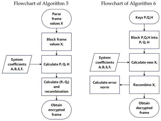
Figure 1. Flowcharts of Algorithms 5 and 6.

First, we take a frame from the video and parse its pixel data. We divide the $480\times 480$ frame into 3600 $3\times 3$ subblocks. Then, we set the coefficients $A_i,B_i,E_i,F_i$ by generating random matrices. We calculate $P_i,Q_i,H$ for each subblock. We take $(P_i-Q_i)$ as the cryptographic subblock corresponding to each subblock. Then, $(P_i-Q_i)$ is restored to the corresponding position and the encrypted frame is generated. The decryption process is that the input coefficients $A_i,B_i,E_i,F_i,P_i,Q_i,H$ calculate the new subblock $X_i$ and then it is restored according to the corresponding position to generate the decrypted frame. Then, we calculate that the decrypted frame has a good restoration effect with the original frame.

Algorithm 5 Block Encryption Process of Frame

(1) Input: one original frame and system coefficients $A_1,A_2,\dots ,A_n,B_1,B_2,\dots ,B_n,$ $E_1,E_2,\dots ,E_n$ and $F_1,F_2,\dots ,F_n\in {\mathbb{Q}}_S^{3\times 3}$. (2) Parse the frames: $X\in {\mathbb{Q}}_S^{480\times 480}$ represents the frame and $X_i\in {\mathbb{Q}}_S^{3\times 3}$ represents the i-th sub-frame of the frame where $i=1,\dots ,n$. (3) Calculate the matrices $P_1,P_2,\dots ,P_n,Q_1,Q_2,\dots ,Q_n\in {\mathbb{Q}}_S^{3\times 3}$ and $H\in {\mathbb{Q}}_S^{3\times 3}$ by system (1). (4) Assemble the i-th sub-frame $X_i,P_i,Q_i$ where $i=1,\dots ,n$ back into the frame $X,P,Q\in {\mathbb{Q}}_S^{480\times 480}$. Encrypt the frame X by $(P-Q)\in {\mathbb{Q}}_S^{480\times 480}$. (5) Output: Encrypted frame.

Algorithm 6 Block Decryption Process of Frame

(1) Input: Encrypted frame $X\in {\mathbb{Q}}_S^{480\times 480}$, keys $P,Q,H\in {\mathbb{Q}}_S^{480\times 480}$ and system coefficients $A_i,B_i,E_i,F_i\in {\mathbb{Q}}_S^{3\times 3}$ where $i=1,\dots ,n$. (2) Calculate the matrices $[\dot{X_1},\dot{X_2},\dots ,\dot{X_n}]$ by Algorithm 1. (3) Recover the frame: $\dot{X_i}\in {\mathbb{Q}}_S^{3\times 3}$ represents the i-th recovered sub-frame where $i=1,\dots ,n$; assemble the $\dot{X_i}$ back into the frame $\dot{X}\in {\mathbb{Q}}_S^{480\times 480}$. (4) Calculate the error norm between X and $\dot{X}$. (5) Output: Decrypted frame.

Remark 1. 

As the dimensions of the decrypted video increase, the time and space complexity of Algorithms 3 and 4 increase exponentially. Therefore, we propose a block encryption and decryption algorithm in Algorithms 5 and 6. By reusing Algorithms 5 and 6, the memory usage can be reduced and the operational speed can be significantly enhanced. It is worth mentioning that Algorithms 5 and 6 are also suitable for local encryption and decryption tasks.

All numerical experiments in this paper were performed in the following hardware and software configurations: Intel(R) Core(TM) i5-10210U CPU @ 1.60 GHz 2.11 GHz, 16 GB RAM, Windows 11 operating system, and MATLAB R2018a. In addition, all test videos were taken using the author’s camera.

Example 2. 

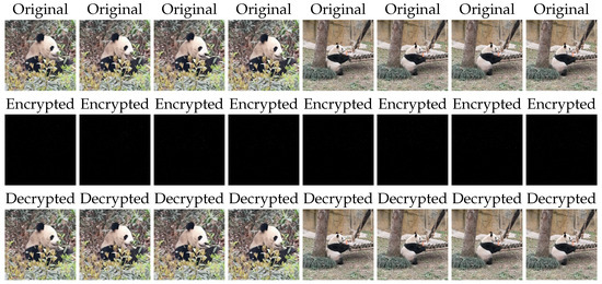
Let us input two videos and execute the above algorithms. The following is the result using MATLAB (Figure 2):

Figure 2. Frames before and after Encryption and Decryption.

In the result, the average error between the numerical solution and the true solution is $2.7106\times {10}^{-9}$. The error of each frame is shown in Table 1 as follows.

Table 1. Error between numerical solution and true solution.

Video 1	Error	Video 2	Error
1-frame	$2.6377\times {10}^{-9}$	1-frame	$2.7776\times {10}^{-9}$
10-frame	$2.6527\times {10}^{-9}$	10-frame	$2.7644\times {10}^{-9}$
16-frame	$2.6655\times {10}^{-9}$	16-frame	$2.7569\times {10}^{-9}$
25-frame	$2.6595\times {10}^{-9}$	25-frame	$2.7707\times {10}^{-9}$

To further evaluate the quality of the decrypted videos, we use the Peak Signal-to-Noise Ratio (PSNR), Structural Similarity Index (SSIM), and Feature Similarity Index (FSIM) [31]. The results are summarized in Table 2. All PSNR values exceed 50, while both SSIM and FSIM values are 1, demonstrating the outstanding quality of our decrypted videos.

Table 2. PSNR, SSIM, and FSIM of video 1 and video 2.

Video 1	PSNR	SSIM	FSIM	Video 2	PSNR	SSIM	FSIM
1-frame	245.4833	1	1	1-frame	244.6598	1	1
10-frame	246.1960	1	1	10-frame	245.8679	1	1
16-frame	246.0469	1	1	16-frame	245.6220	1	1
25-frame	246.0457	1	1	25-frame	245.4920	1	1

Example 3. 

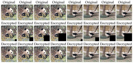
Let us input two videos and finish local encryption and decryption using Algorithms 5 and 6 with MATLAB (Figure 3):

Figure 3. Frames before and after Block Encryption and Decryption.

In the result, the average error between the numerical solution and the true solution is $8.9857\times {10}^{-10}$. The error of each frame is listed in Table 3 as follows.

Table 3. Error between numerical solution and true solution.

Video 1	Error	Video 2	Error
3-frame	$4.0604\times {10}^{-10}$	3-frame	$4.1622\times {10}^{-10}$
12-frame	$8.4663\times {10}^{-10}$	12-frame	$7.7403\times {10}^{-10}$
18-frame	$1.1171\times {10}^{-9}$	18-frame	$9.9505\times {10}^{-10}$
27-frame	$1.4076\times {10}^{-9}$	27-frame	$1.2259\times {10}^{-9}$

The results of PSNR, SSIM, and FSIM are shown in Table 4. PSNR values all exceed 50, while both SSIM and FSIM values reach 1, indicating that the quality of local decryption is excellent.

Table 4. PSNR, SSIM, and FSIM of video 1 and video 2.

Video 1	PSNR	SSIM	FSIM	Video 2	PSNR	SSIM	FSIM
3-frame	245.0190	1	1	3-frame	244.3713	1	1
12-frame	244.5530	1	1	12-frame	244.8359	1	1
18-frame	244.6391	1	1	18-frame	246.7069	1	1
27-frame	245.3403	1	1	27-frame	246.3910	1	1

6. Conclusions

The system of quaternion tensor equation (1) is universal, encompassing many other systems. This kind of system of quaternion tensor equations has practical applications in many areas. In this paper, we first transformed the quaternion tensor equations into quaternion matrix equations through the function f. By using the complex representation of split quaternion matrices and Moore–Penrose inverse, we presented a necessary and sufficient condition for the existence of a general solution to system (1). When the solvability conditions hold, we also derived the expression of the general solution to system (1). In particular, the unique solution was also given when the uniqueness condition held. Then, we converted the obtained quaternion matrix solution back into a quaternion tensor solution using the function $f^{-1}$. Additionally, we established two algorithms to solve system (1), and one example was given to prove the correctness of our results. In the last part, we provided the algorithms and two examples for color video encryption and decryption using the obtained results of system (1). To the best of our knowledge, a substantial body of excellent work has been dedicated to the encryption and decryption of color images. For instance, Feng et al. [32,33,34,35] have put forward numerous effective algorithms for color image encryption and decryption. Kong et al. [36] realized image encryption on a Field-Programmable Gate Array (FPGA). Similarly, Yu et al. [37] developed a system that was implemented on an FPGA digital hardware platform. Moving forward, we will concentrate on some systems of tensor equations over the split quaternion algebra and delve deeper into the study of encryption and decryption.

References

- Hamilton, W.R. Lectures on Quaternions; Hodges and Smith: Dublin, Ireland, 1853. [Google Scholar]
- Took, C.C.; Mandic, D.P. Augmented second-order statistics of quaternion random signals. Signal Process. 2011, 91, 214–224. [Google Scholar] [CrossRef]
- Miao, J.; Kou, K.I. Color image recovery using low-rank quaternion matrix completion algorithm. IEEE Trans. Image Process. 2021, 31, 190–201. [Google Scholar] [CrossRef]
- Jia, Z.G.; Ling, S.T.; Zhao, M.X. Color two-dimensional principal component analysis for face recognition based on quaternion model. In Intelligent Computing Theories and Application: Proceedings of the 13th International Conference, Liverpool, UK, 7–10 August 2017; Springer: Cham, Switzerland, 2017; pp. 177–189. [Google Scholar] [CrossRef]
- Cockle, J. LII. On systems of algebra involving more than one imaginary; and on equations of the fifth degree. Lond. Edinb. Dublin Philos. Mag. J. Sci. 1849, 35, 434–437. [Google Scholar] [CrossRef]
- Adler, S.L. Quaternionic Quantum Mechanics and Quantum Fields; Oxford University Press: Cary, NC, USA, 1995. [Google Scholar]
- Shoemake, K. Animating rotation with quaternion curves. ACM SIGGRAPH Comput. Graph. 1985, 19, 245–254. [Google Scholar] [CrossRef]
- Antonelli, G.; Chiaverini, S. Fault tolerant kinematic control of platoons of autonomous vehicles. IEEE Int. Conf. Robot. Autom. 2004, 4, 3313–3318. [Google Scholar] [CrossRef]
- Krizhevsky, A.; Sutskever, I.; Hinton, G.E. Imagenet classification with deep convolutional neural networks. Commun. ACM 2017, 60, 84–90. [Google Scholar] [CrossRef]
- Carroll, S.M. Spacetime and Geometry: An Introduction to General Relativity, 2nd ed.; Cambridge University Press: Cambridge, UK, 2019. [Google Scholar]
- Griffiths, D.J.; Heald, M.A. Introduction to Electrodynamics, 4th ed.; Cambridge University Press: Cambridge, UK, 2013. [Google Scholar]
- Abadi, M.; Barham, P.; Chen, J.; Chen, Z.; Davis, A.; Dean, J.; Zheng, X. Tensorflow: A system for large-scale machine learning. In 12th USENIX Symposium on Operating Systems Design and Implementation, OSDI 16; USENIX Association: Savannah, GA, USA, 2016; pp. 265–283. [Google Scholar]
- Paszke, A.; Gross, S.; Massa, F.; Lerer, A.; Bradbury, J.; Chanan, G.; Chintala, S. Pytorch: An imperative style, high-performance deep learning library. Adv. Neural Inf. Process. Syst. 2019, 32, 8026–8037. [Google Scholar]
- Zhang, S.; Yao, L.; Sun, A.; Tay, Y. Deep learning based recommender system: A survey and new perspectives. ACM Comput. Surv. 2019, 52, 1–38. [Google Scholar] [CrossRef]
- Qi, L.Q.; Luo, Z.Y. Tensor Analysis: Spectral Theory and Special Tensors; Society for Industrial & Applied Mathematics: Philadelphia, PA, USA, 2017. [Google Scholar]
- Qi, L.Q. Tensor Eigenvalues and Their Applications; Springer Nature: Singapore, 2018. [Google Scholar]
- Ding, W.Y.; Luo, Z.Y.; Qi, L.Q. P-tensors, P0-tensors, and their applications. Linear Algebra Appl. 2018, 555, 336. [Google Scholar] [CrossRef]
- He, Z.H.; Wang, X.X.; Zhao, Y.F. Eigenvalues of quaternion tensors with applications to color video processing. J. Sci. Comput. 2023, 94, 1. [Google Scholar] [CrossRef]
- He, Z.H.; Liu, T.T.; Wang, X.X. Eigenvalues of quaternion tensors: Properties, algorithms and applications. Adv. Appl. Clifford Algebr. 2025, 35, 4. [Google Scholar] [CrossRef]
- Zhang, X.F.; Zhang, W.D.; Li, T. Tensor form of GPBiCG algorithm for solving the generalized Sylvester quaternion tensor equations. J. Franklin Inst. 2023, 360, 5929–5946. [Google Scholar] [CrossRef]
- Zhang, X.F.; Li, T.; Ou, Y.G. Iterative solutions of generalized sylvester quaternion tensor equations. Linear Multilinear Algebra 2023, 72, 1259–1278. [Google Scholar] [CrossRef]
- Gao, Z.H.; Wang, Q.W.; Xie, L.M. The (anti-)η-hermitian solution to a novel system of matrix equations over the split quaternion algebra. Math. Methods Appl. Sci. 2024, 47, 13896–13913. [Google Scholar] [CrossRef]
- Xie, M.Y.; Wang, Q.W.; Zhang, Y. The BiCG algorithm for solving the minimal frobenius norm solution of generalized sylvester tensor equation over the quaternions. Symmetry 2024, 16, 1167. [Google Scholar] [CrossRef]
- Yang, L.Q.; Wang, Q.W.; Kou, Z. A system of tensor equations over the dual split quaternion algebra with an application. Mathematics 2024, 12, 3571. [Google Scholar] [CrossRef]
- Sun, L.Z.; Zheng, B.D.; Bu, C.J.; Wei, Y.M. Moore–Penrose inverse of tensors via Einstein product. Linear Multilinear Algebra 2016, 64, 686–698. [Google Scholar] [CrossRef]
- Liu, T.T.; Yu, S.W. Some properties of reduced biquaternion tensors. Symmetry 2024, 16, 1260. [Google Scholar] [CrossRef]
- Yuan, S.F.; Wang, Q.W.; Yu, Y.B.; Tian, Y. On hermitian solutions of the split quaternion matrix equation AXB + CXD = E. Adv. Appl. Clifford Algebras 2017, 27, 3235–3252. [Google Scholar] [CrossRef]
- Ben-Israel, A.; Greville, T.N.E. Generalized Inverses: Theory and Applications; Springer Science & Business Media: New York, NY, USA, 2006. [Google Scholar]
- Magnus, J.R. L-structured matrices and linear matrix equations. Linear Multilinear Algebra 1983, 14, 67–88. [Google Scholar] [CrossRef]
- Xie, L.M.; Wang, Q.W. A system of matrix equations over the commutative quaternion ring. Filomat 2023, 37, 97–106. [Google Scholar] [CrossRef]
- Sara, U.; Akter, M.; Uddin, M.S. Image quality assessment through FSIM, SSIM, MSE and PSNR-a comparative study. J. Comput. Commun. 2019, 7, 8–18. [Google Scholar] [CrossRef]
- Feng, W.; Zhang, J.; Qin, Z.T. A secure and efficient image transmission scheme based on two chaotic maps. Complexity 2021, 2021, 1898998. [Google Scholar] [CrossRef]
- Feng, W.; Zhao, X.Y.; Zhang, J.; Qin, Z.T.; Zhang, J.K.; He, Y.G. Image encryption algorithm based on plane-level image filtering and discrete logarithmic transform. Mathematics 2022, 10, 2751. [Google Scholar] [CrossRef]
- Feng, W.; Yang, J.X.; Zhao, X.Y.; Qin, Z.T.; Zhang, J.; Zhu, Z.G.; Wen, H.P.; Qian, K. A novel multi-channel image encryption algorithm leveraging pixel reorganization and hyperchaotic maps. Mathematics 2024, 12, 3917. [Google Scholar] [CrossRef]
- Feng, W.; Zhang, J.; Chen, Y.; Qin, Z.T.; Zhang, Y.S.; Ahmad, M.; Woźniak, M. Exploiting robust quadratic polynomial hyperchaotic map and pixel fusion strategy for efficient image encryption. Expert Syst. Appl. 2024, 246, 123190. [Google Scholar] [CrossRef]
- Kong, X.X.; Yu, F.; Yao, W.; Cai, S.; Zhang, J.; Lin, H.R. Memristor-induced hyperchaos, multiscroll and extreme multistability in fractional-order HNN: Image encryption and FPGA implementation. IEEE Trans. Neural Netw. 2024, 171, 85–103. [Google Scholar] [CrossRef]
- Yu, F.; Lin, Y.; Yao, W.; Cai, S.; Lin, H.R.; Li, Y. Multiscroll hopfield neural network with extreme multistability and its application in video encryption for IIoT. IEEE Trans. Neural Netw. 2025, 182, 106904. [Google Scholar] [CrossRef] [PubMed]
Disclaimer/Publisher’s Note: The statements, opinions and data contained in all publications are solely those of the individual author(s) and contributor(s) and not of MDPI and/or the editor(s). MDPI and/or the editor(s) disclaim responsibility for any injury to people or property resulting from any ideas, methods, instructions or products referred to in the content. |
© 2025 by the authors. Licensee MDPI, Basel, Switzerland. This article is an open access article distributed under the terms and conditions of the Creative Commons Attribution (CC BY) license (https://creativecommons.org/licenses/by/4.0/).