
On the Asymptotic Normality of the Method of Moments Estimators for the Birnbaum–Saunders Distribution with a New Parametrization


Abstract
1. Introduction
2. Method of Moments Estimation for the Parameters of Birnbaum–Saunders Distribution
3. On the Joint Asymptotic Normality of the Method of Moments Estimators of the Parameters of the Birnbaum–Saunders Distribution
- The estimator is asymptotically normal with mean (asymptotically unbiased) and variance . This is an asymptotic result; it implies that
- The estimator is asymptotically normal with mean (asymptotically unbiased) and variance . This is an asymptotic result; it implies that
- The covariance of the method of moments estimators and is
4. Simulation Study
- Algorithm 1. Step 0. Fix and .
- Algorithm 2. Step i. Simulate N samples of size n of random numbers that follow the Birnbaum–Saunders distribution with parameters and by Algorithm 1.
4.1. Scope
4.2. Comparing the Simulation and Theoretical Results
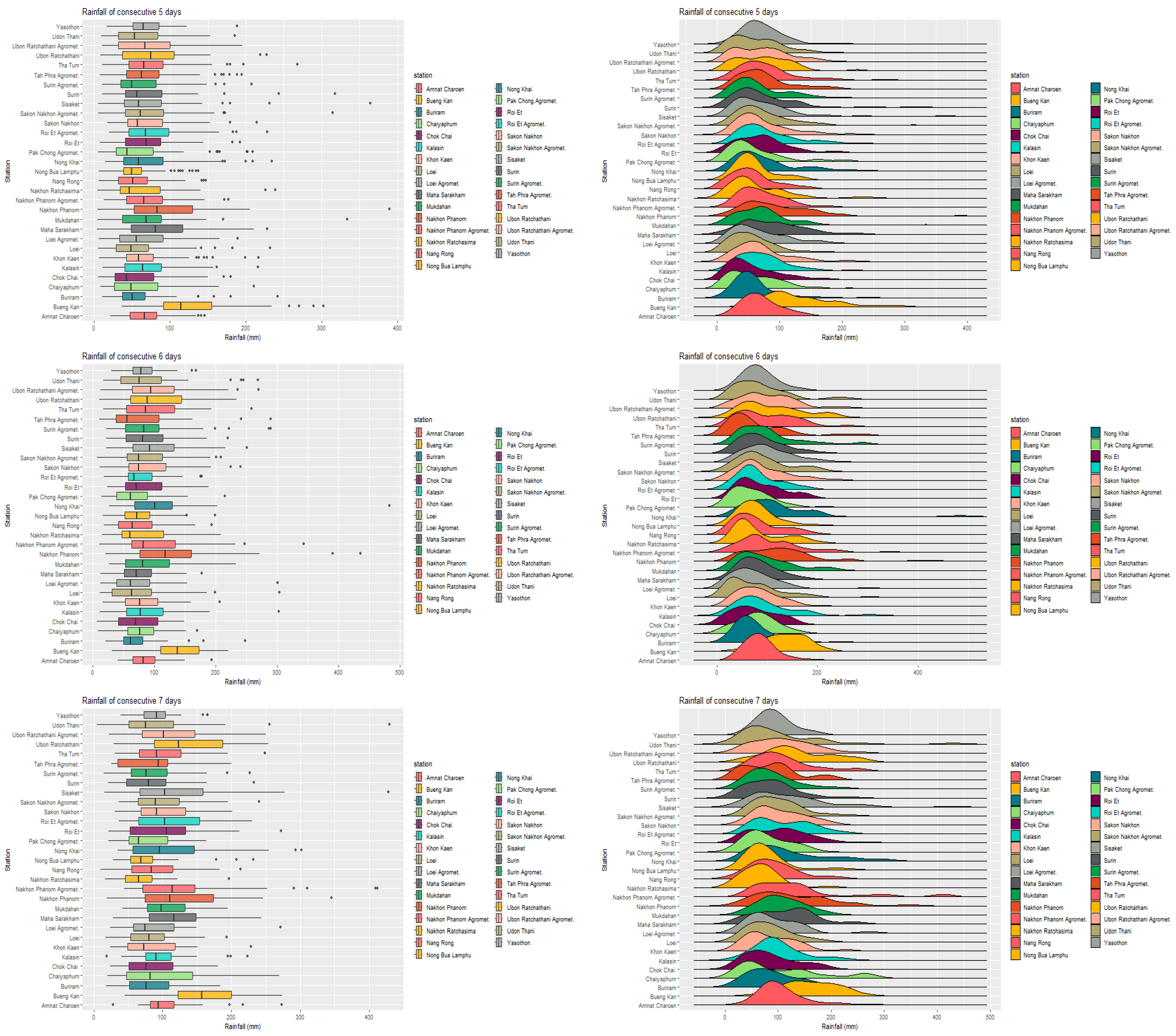
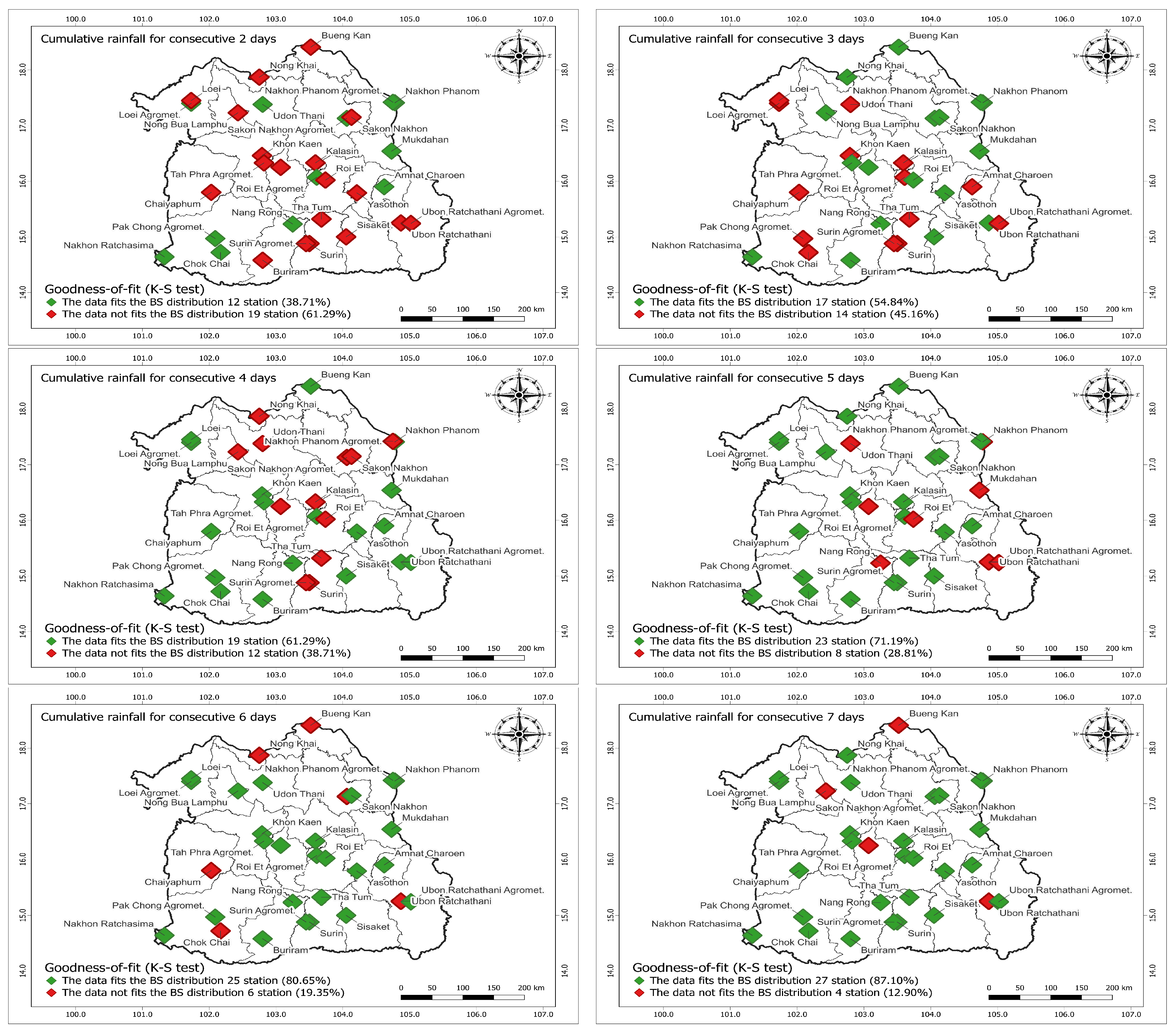
5. Real-Life Example
6. Return Level of Birnbaum–Saunders Distribution
7. Discussion
8. Conclusions
Author Contributions
Funding
Data Availability Statement
Acknowledgments
Conflicts of Interest
References
- Birnbaum, Z.W.; Saunders, S.C. A new family of the life distribution. J. Appl. Probab. 1969, 6, 319–327. [Google Scholar] [CrossRef]
- Leiva, V. The Birnbaum-Saunders Distribution; Academic Press: Cambridge, MA, USA, 2015. [Google Scholar]
- Ahmed, S.E.; Budsaba, K.; Lisawadi, S.; Volodin, A. Parametric estimation for the Birnbaum-Saunders lifetime distribution based on a new parametrization. Thail. Stat. 2008, 6, 213–240. [Google Scholar]
- Balakrishnan, N.; Zhu, X. An improved method of estimation for the parameters of the Birnbaum-Saunders distribution. J. Stat. Comput. Simul. 2014, 84, 2285–2294. [Google Scholar] [CrossRef]
- Ng, H.K.T.; Kundu, D.; Balakrishnan, N. Modified moment estimation for the two-parameter Birnbaum-Saunders distribution. Comput. Stat. Data Anal. 2003, 43, 283–298. [Google Scholar] [CrossRef]
- Zhang, J.; Chen, W.; Yang, R. Birnbaum-Saunders parameters estimation using simple random sampling and ranked set sampling. Commun. Stat.-Simul. Comput. 2024, 1–20. [Google Scholar] [CrossRef]
- Cramér, H. Mathematical Methods of Statistics; Princeton University Press: Princeton, NJ, USA, 2016. [Google Scholar]
- Lehmann, E. Elements of Large Sample Theory; Springer Science & Business Media: Cham, Switzerland, 2004. [Google Scholar]
- Sawlan, Z.; Scavino, M.; Tempone, R. Modeling metallic fatigue data using the Birnbaum-Saunders distribution. Metals 2024, 14, 508. [Google Scholar] [CrossRef]

| n | Simulation Result | Theoretical Result | ||||||||
|---|---|---|---|---|---|---|---|---|---|---|
| 10 | 0.5 | 0.5 | 0.6058 | 0.6053 | 0.0576 | 0.0590 | 0.0063 | 0.0236 | 0.0236 | 0.0014 |
| 10 | 0.5 | 1 | 0.5960 | 1.1951 | 0.0429 | 0.1757 | 0.0250 | 0.0203 | 0.0813 | 0.0094 |
| 10 | 0.5 | 5 | 0.5815 | 5.8192 | 0.0289 | 2.8181 | 0.2101 | 0.0148 | 1.4757 | 0.1024 |
| 10 | 0.5 | 10 | 0.5805 | 11.6205 | 0.0269 | 10.8728 | 0.4825 | 0.0137 | 5.4752 | 0.2262 |
| 10 | 1 | 0.5 | 1.1878 | 0.5954 | 0.1669 | 0.0428 | 0.0264 | 0.0813 | 0.0203 | 0.0094 |
| 10 | 1 | 1 | 1.1778 | 1.1707 | 0.1337 | 0.1327 | 0.0746 | 0.0694 | 0.0694 | 0.0306 |
| 10 | 1 | 5 | 1.1595 | 5.8011 | 0.1048 | 2.5920 | 0.4663 | 0.0548 | 1.3688 | 0.2262 |
| 10 | 1 | 10 | 1.1576 | 11.5777 | 0.1025 | 10.2823 | 0.9136 | 0.0524 | 5.2438 | 0.4756 |
| 10 | 5 | 0.5 | 5.7873 | 0.5821 | 2.7430 | 0.0280 | 0.2300 | 1.4757 | 0.0148 | 0.1024 |
| 10 | 5 | 1 | 5.8103 | 1.1606 | 2.6498 | 0.1037 | 0.4630 | 1.3688 | 0.0548 | 0.2262 |
| 10 | 5 | 5 | 5.8025 | 5.8011 | 2.5626 | 2.5756 | 2.6054 | 1.2748 | 1.2748 | 1.2252 |
| 10 | 5 | 10 | 5.7804 | 11.5464 | 2.4573 | 9.7477 | 4.8360 | 1.2624 | 5.0498 | 2.4751 |
| 10 | 10 | 0.5 | 11.5864 | 0.5779 | 10.4475 | 0.0258 | 0.4549 | 5.4752 | 0.0137 | 0.2262 |
| 10 | 10 | 1 | 11.5590 | 1.1558 | 10.1876 | 0.1014 | 0.9656 | 5.2438 | 0.0524 | 0.4756 |
| 10 | 10 | 5 | 11.5118 | 5.7584 | 9.7821 | 2.4553 | 4.9364 | 5.0498 | 1.2624 | 2.4751 |
| 10 | 10 | 10 | 11.5277 | 11.5258 | 9.8778 | 9.9101 | 9.9482 | 5.0249 | 5.0249 | 4.9751 |
| 30 | 0.5 | 0.5 | 0.5303 | 0.5302 | 0.0103 | 0.0101 | 0.0008 | 0.0079 | 0.0079 | 0.0005 |
| 30 | 0.5 | 1 | 0.5275 | 1.0538 | 0.0086 | 0.0345 | 0.0045 | 0.0068 | 0.0271 | 0.0031 |
| 30 | 0.5 | 5 | 0.5234 | 5.2413 | 0.0059 | 0.5825 | 0.0432 | 0.0049 | 0.4919 | 0.0341 |
| 30 | 0.5 | 10 | 0.5233 | 10.4598 | 0.0056 | 2.2367 | 0.0903 | 0.0046 | 1.8251 | 0.0754 |
| 30 | 1 | 0.5 | 1.0552 | 0.5248 | 0.0344 | 0.0083 | 0.0042 | 0.0271 | 0.0068 | 0.0031 |
| 30 | 1 | 1 | 1.0541 | 1.0521 | 0.0295 | 0.0294 | 0.0136 | 0.0231 | 0.0231 | 0.0102 |
| 30 | 1 | 5 | 1.0456 | 5.2327 | 0.0224 | 0.5526 | 0.0964 | 0.0183 | 0.4563 | 0.0754 |
| 30 | 1 | 10 | 1.0448 | 10.4456 | 0.0211 | 2.0734 | 0.1973 | 0.0175 | 1.7479 | 0.1585 |
| 30 | 5 | 0.5 | 5.2448 | 0.5245 | 0.6098 | 0.0060 | 0.0420 | 0.4919 | 0.0049 | 0.0341 |
| 30 | 5 | 1 | 5.2429 | 1.0476 | 0.5827 | 0.0238 | 0.0934 | 0.4563 | 0.0183 | 0.0754 |
| 30 | 5 | 5 | 5.2192 | 5.2167 | 0.5199 | 0.5261 | 0.5042 | 0.4249 | 0.4249 | 0.4084 |
| 30 | 5 | 10 | 5.2093 | 10.4164 | 0.4925 | 1.9749 | 1.0392 | 0.4208 | 1.6833 | 0.8250 |
| 30 | 10 | 0.5 | 10.4333 | 0.5223 | 2.1690 | 0.0055 | 0.0889 | 1.8251 | 0.0046 | 0.0754 |
| 30 | 10 | 1 | 10.4290 | 1.0431 | 2.1484 | 0.0214 | 0.1911 | 1.7479 | 0.0175 | 0.1585 |
| 30 | 10 | 5 | 10.4637 | 5.2302 | 2.1203 | 0.5264 | 1.0212 | 1.6833 | 0.4208 | 0.8250 |
| 30 | 10 | 10 | 10.4623 | 10.4624 | 2.0842 | 2.0807 | 2.0807 | 1.6750 | 1.6750 | 1.6584 |
| n | Simulation Result | Theoretical Result | ||||||||
|---|---|---|---|---|---|---|---|---|---|---|
| 50 | 0.5 | 0.5 | 0.5177 | 0.5183 | 0.0055 | 0.0057 | 0.0002 | 0.0047 | 0.0047 | 0.0003 |
| 50 | 0.5 | 1 | 0.5146 | 1.0325 | 0.0046 | 0.0186 | 0.0023 | 0.0041 | 0.0163 | 0.0019 |
| 50 | 0.5 | 5 | 0.5143 | 5.1367 | 0.0033 | 0.3291 | 0.0230 | 0.003 | 0.2951 | 0.0205 |
| 50 | 0.5 | 10 | 0.5137 | 10.2578 | 0.0031 | 1.2049 | 0.0500 | 0.0027 | 1.095 | 0.0452 |
| 50 | 1 | 0.5 | 1.0348 | 0.5158 | 0.0191 | 0.0046 | 0.0023 | 0.0163 | 0.0041 | 0.0019 |
| 50 | 1 | 1 | 1.0294 | 1.0305 | 0.0157 | 0.0161 | 0.0068 | 0.0139 | 0.0139 | 0.0061 |
| 50 | 1 | 5 | 1.0257 | 5.1319 | 0.012 | 0.2996 | 0.0520 | 0.011 | 0.2738 | 0.0452 |
| 50 | 1 | 10 | 1.0272 | 10.2731 | 0.0118 | 1.197 | 0.1100 | 0.0105 | 1.0488 | 0.0951 |
| 50 | 5 | 0.5 | 5.1385 | 0.5136 | 0.3344 | 0.0034 | 0.0229 | 0.2951 | 0.003 | 0.0205 |
| 50 | 5 | 1 | 5.1359 | 1.0261 | 0.2992 | 0.0124 | 0.0516 | 0.2738 | 0.011 | 0.0452 |
| 50 | 5 | 5 | 5.1398 | 5.1381 | 0.289 | 0.2886 | 0.2707 | 0.255 | 0.255 | 0.2450 |
| 50 | 5 | 10 | 5.1296 | 10.2574 | 0.2866 | 1.1452 | 0.5580 | 0.2525 | 1.0100 | 0.4950 |
| 50 | 10 | 0.5 | 10.2679 | 0.5134 | 1.207 | 0.0031 | 0.0530 | 1.095 | 0.0027 | 0.0452 |
| 50 | 10 | 1 | 10.2506 | 1.0252 | 1.179 | 0.0118 | 0.1089 | 1.0488 | 0.0105 | 0.0951 |
| 50 | 10 | 5 | 10.2621 | 5.1311 | 1.1119 | 0.2772 | 0.5506 | 1.01 | 0.2525 | 0.4950 |
| 50 | 10 | 10 | 10.2627 | 10.2612 | 1.1212 | 1.1184 | 1.1087 | 1.005 | 1.005 | 0.9950 |
| 100 | 0.5 | 0.5 | 0.5081 | 0.5086 | 0.0026 | 0.0026 | 0.0002 | 0.0024 | 0.0024 | 0.0001 |
| 100 | 0.5 | 1 | 0.5084 | 1.0162 | 0.0022 | 0.0085 | 0.0011 | 0.002 | 0.0081 | 0.0009 |
| 100 | 0.5 | 5 | 0.5075 | 5.0737 | 0.0016 | 0.1591 | 0.0109 | 0.0015 | 0.1476 | 0.0102 |
| 100 | 0.5 | 10 | 0.5068 | 10.1391 | 0.0015 | 0.5934 | 0.0242 | 0.0014 | 0.5475 | 0.0226 |
| 100 | 1 | 0.5 | 1.0151 | 0.5078 | 0.0086 | 0.0022 | 0.0011 | 0.0081 | 0.002 | 0.0009 |
| 100 | 1 | 1 | 1.0136 | 1.0136 | 0.0075 | 0.0073 | 0.0033 | 0.0069 | 0.0069 | 0.0031 |
| 100 | 1 | 5 | 1.0132 | 5.0704 | 0.0058 | 0.1464 | 0.0247 | 0.0055 | 0.1369 | 0.0226 |
| 100 | 1 | 10 | 1.0137 | 10.1363 | 0.0056 | 0.5499 | 0.0510 | 0.0052 | 0.5244 | 0.0476 |
| 100 | 5 | 0.5 | 5.0661 | 0.5064 | 0.1556 | 0.0016 | 0.0108 | 0.1476 | 0.0015 | 0.0102 |
| 100 | 5 | 1 | 5.0681 | 1.0127 | 0.1477 | 0.0059 | 0.0237 | 0.1369 | 0.0055 | 0.0226 |
| 100 | 5 | 5 | 5.0627 | 5.0622 | 0.1356 | 0.1358 | 0.1309 | 0.1275 | 0.1275 | 0.1225 |
| 100 | 5 | 10 | 5.0661 | 10.1301 | 0.1344 | 0.5377 | 0.2619 | 0.1262 | 0.505 | 0.2475 |
| 100 | 10 | 0.5 | 10.138 | 0.5066 | 0.581 | 0.0014 | 0.0244 | 0.5475 | 0.0014 | 0.0226 |
| 100 | 10 | 1 | 10.1329 | 1.013 | 0.5487 | 0.0054 | 0.0507 | 0.5244 | 0.0052 | 0.0476 |
| 100 | 10 | 5 | 10.12 | 5.0606 | 0.5347 | 0.1339 | 0.2657 | 0.505 | 0.1262 | 0.2475 |
| 100 | 10 | 10 | 10.1176 | 10.1178 | 0.5205 | 0.5237 | 0.5217 | 0.5025 | 0.5025 | 0.4975 |
| n | Simulation Result | Theoretical Result | ||||||||
|---|---|---|---|---|---|---|---|---|---|---|
| 200 | 0.5 | 0.5 | 0.5016 | 0.5016 | 0.0005 | 0.0005 | 0.0001 | 0.0005 | 0.0005 | 0.0001 |
| 200 | 0.5 | 1 | 0.5017 | 1.0036 | 0.0004 | 0.0016 | 0.0005 | 0.0004 | 0.0016 | 0.0005 |
| 200 | 0.5 | 5 | 0.5014 | 5.0132 | 0.0003 | 0.0295 | 0.0054 | 0.0003 | 0.0295 | 0.0051 |
| 200 | 0.5 | 10 | 0.5013 | 10.0281 | 0.0003 | 0.1121 | 0.0121 | 0.0003 | 0.1095 | 0.0113 |
| 200 | 1 | 0.5 | 1.0039 | 0.5017 | 0.0017 | 0.0004 | 0.0005 | 0.0016 | 0.0004 | 0.0005 |
| 200 | 1 | 1 | 1.0028 | 1.0029 | 0.0014 | 0.0014 | 0.0016 | 0.0014 | 0.0014 | 0.0015 |
| 200 | 1 | 5 | 1.0028 | 5.0154 | 0.0011 | 0.0284 | 0.0118 | 0.0011 | 0.0274 | 0.0113 |
| 200 | 1 | 10 | 1.0024 | 10.0265 | 0.0011 | 0.1083 | 0.0245 | 0.001 | 0.1049 | 0.0238 |
| 200 | 5 | 0.5 | 5.0149 | 0.5013 | 0.0299 | 0.0003 | 0.0054 | 0.0295 | 0.0003 | 0.0051 |
| 200 | 5 | 1 | 5.0133 | 1.0031 | 0.0271 | 0.0011 | 0.0115 | 0.0274 | 0.0011 | 0.0113 |
| 200 | 5 | 5 | 5.0119 | 5.0123 | 0.0261 | 0.0262 | 0.0642 | 0.0255 | 0.0255 | 0.0613 |
| 200 | 5 | 10 | 5.0152 | 10.0296 | 0.0264 | 0.1052 | 0.1277 | 0.0252 | 0.101 | 0.1238 |
| 200 | 10 | 0.5 | 10.0263 | 0.5014 | 0.1116 | 0.0003 | 0.0118 | 0.1095 | 0.0003 | 0.0113 |
| 200 | 10 | 1 | 10.0239 | 1.0023 | 0.1065 | 0.0011 | 0.0240 | 0.1049 | 0.001 | 0.0238 |
| 200 | 10 | 5 | 10.0219 | 5.011 | 0.1025 | 0.0257 | 0.1328 | 0.101 | 0.0252 | 0.1238 |
| 200 | 10 | 10 | 10.0297 | 10.0297 | 0.102 | 0.1018 | 0.2502 | 0.1005 | 0.1005 | 0.2488 |
| 500 | 0.5 | 0.5 | 0.5008 | 0.5007 | 0.0002 | 0.0002 | 0.0000 | 0.0002 | 0.0002 | 0.0000 |
| 500 | 0.5 | 1 | 0.5006 | 1.0016 | 0.0002 | 0.0008 | 0.0002 | 0.0002 | 0.0008 | 0.0002 |
| 500 | 0.5 | 5 | 0.5007 | 5.0057 | 0.0001 | 0.0147 | 0.0021 | 0.0001 | 0.0148 | 0.0020 |
| 500 | 0.5 | 10 | 0.5006 | 10.0107 | 0.0001 | 0.0543 | 0.0045 | 0.0001 | 0.0548 | 0.0045 |
| 500 | 1 | 0.5 | 1.0016 | 0.5008 | 0.0008 | 0.0002 | 0.0002 | 0.0008 | 0.0002 | 0.0002 |
| 500 | 1 | 1 | 1.0017 | 1.0013 | 0.0007 | 0.0007 | 0.0006 | 0.0007 | 0.0007 | 0.0006 |
| 500 | 1 | 5 | 1.0016 | 5.0074 | 0.0006 | 0.0137 | 0.0045 | 0.0005 | 0.0137 | 0.0045 |
| 500 | 1 | 10 | 1.0018 | 10.0171 | 0.0005 | 0.0521 | 0.0095 | 0.0005 | 0.0524 | 0.0095 |
| 500 | 5 | 0.5 | 5.0061 | 0.5006 | 0.0147 | 0.0002 | 0.0021 | 0.0148 | 0.0001 | 0.0020 |
| 500 | 5 | 1 | 5.0079 | 1.0015 | 0.0138 | 0.0006 | 0.0046 | 0.0137 | 0.0005 | 0.0045 |
| 500 | 5 | 5 | 5.0061 | 5.0065 | 0.0127 | 0.0128 | 0.0251 | 0.0127 | 0.0127 | 0.0245 |
| 500 | 5 | 10 | 5.0072 | 10.0148 | 0.0125 | 0.05 | 0.0497 | 0.0126 | 0.0505 | 0.0495 |
| 500 | 10 | 0.5 | 10.0137 | 0.5006 | 0.0544 | 0.0001 | 0.0046 | 0.0548 | 0.0001 | 0.0045 |
| 500 | 10 | 1 | 10.0138 | 1.0015 | 0.052 | 0.0005 | 0.0097 | 0.0524 | 0.0005 | 0.0095 |
| 500 | 10 | 5 | 10.0101 | 5.0053 | 0.0512 | 0.0128 | 0.0509 | 0.0505 | 0.0126 | 0.0495 |
| 500 | 10 | 10 | 10.0137 | 10.0137 | 0.0517 | 0.0518 | 0.0994 | 0.0502 | 0.0502 | 0.0995 |
| Data | ID | Station | n | L-limit () | U-limit () | L-limit () | U-limit () | ||
|---|---|---|---|---|---|---|---|---|---|
| CONS-2 | 48350 | Loei Agromet | 402 | 2.428 | 2.266 | 2.590 | 5.106 | 4.871 | 5.341 |
| 48354 | Udon Thani | 358 | 2.290 | 2.123 | 2.456 | 10.202 | 9.851 | 10.553 | |
| 48357 | Nakhon Phanom | 332 | 2.568 | 2.386 | 2.751 | 13.061 | 12.649 | 13.473 | |
| 48391 | Amnat Charoen | 372 | 6.548 | 6.273 | 6.822 | 15.236 | 14.817 | 15.655 | |
| 48431 | Nakhon Ratchasima | 439 | 2.240 | 2.091 | 2.388 | 8.583 | 8.292 | 8.874 | |
| CONS-3 | 48352 | Nong Khai | 207 | 0.185 | 0.117 | 0.253 | 4.742 | 4.398 | 5.085 |
| 48357 | Nakhon Phanom | 188 | 0.179 | 0.109 | 0.250 | 4.468 | 4.116 | 4.821 | |
| 48383 | Mukdahan | 204 | 0.189 | 0.120 | 0.257 | 4.862 | 4.512 | 5.212 | |
| 48407 | Ubon Ratchathani | 217 | 0.181 | 0.115 | 0.246 | 5.044 | 4.699 | 5.390 | |
| 48431 | Nakhon Ratchasima | 223 | 0.189 | 0.123 | 0.256 | 4.061 | 3.752 | 4.370 | |
| CONS-4 | 48350 | Loei Agromet | 136 | 0.187 | 0.103 | 0.270 | 6.109 | 5.632 | 6.587 |
| 48357 | Nakhon Phanom | 99 | 0.164 | 0.072 | 0.255 | 7.859 | 7.225 | 8.494 | |
| 48383 | Mukdahan | 113 | 0.209 | 0.114 | 0.303 | 9.313 | 8.680 | 9.946 | |
| 48407 | Ubon Ratchathani | 117 | 0.192 | 0.102 | 0.282 | 7.942 | 7.362 | 8.522 | |
| 48431 | Nakhon Ratchasima | 114 | 0.178 | 0.088 | 0.268 | 5.814 | 5.301 | 6.327 | |
| CONS-5 | 48350 | Loei Agromet | 93 | 0.183 | 0.084 | 0.282 | 9.183 | 8.484 | 9.883 |
| 48358 | Nakhon Phanom Agromet | 76 | 0.240 | 0.117 | 0.363 | 14.662 | 13.704 | 15.620 | |
| 48363 | Bueng Kan | 83 | 0.214 | 0.105 | 0.323 | 25.197 | 24.010 | 26.385 | |
| 48391 | Amnat Charoen | 88 | 0.284 | 0.161 | 0.406 | 17.781 | 16.812 | 18.749 | |
| 48431 | Nakhon Ratchasima | 69 | 0.181 | 0.065 | 0.296 | 8.264 | 7.483 | 9.045 | |
| CONS-6 | 48350 | Loei Agromet | 66 | 0.188 | 0.069 | 0.307 | 10.674 | 9.776 | 11.571 |
| 48357 | Nakhon Phanom | 55 | 0.146 | 0.031 | 0.261 | 15.322 | 14.141 | 16.503 | |
| 48383 | Mukdahan | 51 | 0.191 | 0.055 | 0.327 | 15.111 | 13.900 | 16.322 | |
| 48408 | Ubon Ratchathani Agromet | 48 | 0.161 | 0.030 | 0.291 | 13.300 | 12.114 | 14.486 | |
| 48431 | Nakhon Ratchasima | 41 | 0.195 | 0.040 | 0.350 | 13.647 | 12.346 | 14.948 | |
| CONS-7 | 48350 | Loei Agromet | 27 | 0.207 | 0.005 | 0.408 | 16.264 | 14.475 | 18.053 |
| 48357 | Nakhon Phanom | 34 | 0.153 | 0.000 | 0.307 | 16.036 | 14.466 | 17.606 | |
| 48383 | Mukdahan | 33 | 0.248 | 0.054 | 0.442 | 24.038 | 22.127 | 25.949 | |
| 48408 | Ubon Ratchathani Agromet | 35 | 0.177 | 0.016 | 0.339 | 16.448 | 14.893 | 18.004 | |
| 48431 | Nakhon Ratchasima | 23 | 0.228 | -0.006 | 0.461 | 13.549 | 11.748 | 15.350 |
| Data | ID | 2 Years | 10 Years | 20 Years | 50 Years | 100 Years |
|---|---|---|---|---|---|---|
| CONS-2 | 48350 | 9.4 (7.6, 11.1) | 41.7 (40.0, 43.5) | 58.6 (56.8, 60.3) | 82.1 (80.4, 83.8) | 100.5 (98.8, 102.3) |
| 48354 | 10.1 (7.7, 12.5) | 51.1 (48.6, 53.5) | 73.0 (70.5, 75.4) | 103.7 (101.3, 106.1) | 127.8 (125.4, 130.2) | |
| 48357 | 12.9 (9.6, 16.1) | 66.4 (63.2, 69.6) | 95.1 (91.9, 98.3) | 135.4 (132.1, 138.6) | 167 (163.8, 170.2) | |
| 48391 | 21.0 (19.4, 22.7) | 50.3 (48.6, 52.0) | 63.1 (61.4, 64.8) | 80.3 (78.6, 82.0) | 93.5 (91.8, 95.1) | |
| 48431 | 9.6 (7.6, 11.6) | 48.7 (46.8, 50.7) | 69.6 (67.6, 71.6) | 98.9 (96.9, 100.9) | 121.9 (119.9, 123.9) | |
| CONS-3 | 48352 | 25.1 (20.5, 29.7) | 90.1 (85.5, 94.7) | 122.3 (117.7, 126.9) | 166.9 (162.3, 171.4) | 201.6 (197.0, 206.2) |
| 48357 | 24.4 (19.2, 29.6) | 92.4 (87.2, 97.6) | 126.5 (121.3, 131.7) | 173.9 (168.7, 179.1) | 210.8 (205.6, 216.1) | |
| 48383 | 25.6 (20.4, 30.7) | 89.7 (84.6, 94.9) | 121.3 (116.1, 126.5) | 164.9 (159.8, 170.1) | 198.9 (193.8, 204.1) | |
| 48407 | 27.6 (22.4, 32.7) | 97.1 (91.9, 102.2) | 131.3 (126.1, 136.5) | 178.7 (173.5, 183.8) | 215.6 (210.4, 220.7) | |
| 48431 | 21.0 (16.8, 25.1) | 81.3 (77.2, 85.5) | 111.8 (107.6, 116.0) | 154.2 (150.0, 158.4) | 187.3 (183.1, 191.5) | |
| CONS-4 | 48350 | 32.4 (25.9, 39.0) | 101.1 (94.5, 107.6) | 133.8 (127.2, 140.3) | 178.7 (172.1, 185.2) | 213.5 (207.0, 220.1) |
| 48357 | 47.8 (37.2, 58.3) | 140.3 (129.8, 150.9) | 183.7 (173.1, 194.2) | 242.9 (232.3, 253.5) | 288.8 (278.2, 299.3) | |
| 48383 | 44.5 (38.2, 50.8) | 108.3 (101.9, 114.6) | 136.4 (130.0, 142.7) | 174.1 (167.8, 180.4) | 203.1 (196.7, 209.4) | |
| 48407 | 41.2 (33.8, 48.7) | 111.7 (104.3, 119.1) | 143.9 (136.4, 151.3) | 187.5 (180.1, 195.0) | 221.2 (213.8, 228.7) | |
| 48431 | 32.2 (25.1, 39.3) | 105.7 (98.6, 112.7) | 141.2 (134.1, 148.3) | 190.1 (183.0, 197.2) | 228.1 (221, 235.2) | |
| CONS-5 | 48350 | 49.9 (41.4, 58.4) | 129.2 (120.7, 137.8) | 165 (156.5, 173.5) | 213.2 (204.7, 221.7) | 250.4 (241.9, 258.9) |
| 48358 | 61.0 (53.3, 68.8) | 119.3 (111.6, 127.1) | 142.9 (135.2, 150.7) | 173.8 (166, 181.6) | 197.0 (189.3, 204.8) | |
| 48363 | 117.8 (105.8, 129.8) | 203.2 (191.2, 215.2) | 235.9 (223.9, 247.8) | 277.8 (265.8, 289.8) | 308.9 (297, 320.9) | |
| 48391 | 62.7 (56.7, 68.7) | 110.1 (104.1, 116.2) | 128.4 (122.4, 134.5) | 152.0 (146.0, 158.0) | 169.5 (163.5, 175.6) | |
| 48431 | 45.5 (34.9, 56.0) | 124.3 (113.8, 134.9) | 160.4 (149.9, 171.0) | 209.5 (199.0, 220.1) | 247.4 (236.8, 258) | |
| CONS-6 | 48350 | 56.6 (45.4, 67.9) | 136.1 (124.9, 147.3) | 170.9 (159.7, 182.1) | 217.7 (206.5, 228.9) | 253.5 (242.3, 264.7) |
| 48357 | 104.8 (83.4, 126.2) | 241.0 (219.6, 262.5) | 299.8 (278.4, 321.2) | 378.3 (356.9, 399.7) | 438.3 (416.8, 459.7) | |
| 48383 | 79.1 (64.5, 93.7) | 165.4 (150.8, 180.0) | 201.2 (186.6, 215.8) | 248.6 (234.0, 263.2) | 284.5 (269.9, 299.1) | |
| 48408 | 82.3 (66.3, 98.2) | 192.5 (176.5, 208.4) | 240.3 (224.4, 256.2) | 304.4 (288.4, 320.3) | 353.3 (337.4, 369.2) | |
| 48431 | 70.0 (54.6, 85.4) | 150.7 (135.2, 166.1) | 184.6 (169.2, 200.1) | 229.6 (214.2, 245) | 263.8 (248.3, 279.2) | |
| CONS-7 | 48350 | 78.7 (59.1, 98.2) | 156.1 (136.6, 175.6) | 187.6 (168.1, 207.1) | 228.9 (209.4, 248.4) | 260.1 (240.6, 279.6) |
| 48357 | 104.4 (80.5, 128.3) | 231.4 (207.5, 255.3) | 285.5 (261.6, 309.4) | 357.4 (333.5, 381.3) | 412.1 (388.2, 436.0) | |
| 48383 | 96.8 (83.3, 110.3) | 162.6 (149.1, 176.1) | 187.5 (174.0, 201.0) | 219.3 (205.8, 232.8) | 242.8 (229.3, 256.3) | |
| 48408 | 92.6 (74.6, 110.5) | 192.8 (174.9, 210.7) | 234.4 (216.5, 252.3) | 289.3 (271.4, 307.3) | 331.0 (313.0, 348.9) | |
| 48431 | 59.4 (43.8, 74.9) | 121.3 (105.7, 136.8) | 146.8 (131.2, 162.3) | 180.3 (164.8, 195.9) | 205.7 (190.2, 221.3) |
Disclaimer/Publisher’s Note: The statements, opinions and data contained in all publications are solely those of the individual author(s) and contributor(s) and not of MDPI and/or the editor(s). MDPI and/or the editor(s) disclaim responsibility for any injury to people or property resulting from any ideas, methods, instructions or products referred to in the content. |
© 2025 by the authors. Licensee MDPI, Basel, Switzerland. This article is an open access article distributed under the terms and conditions of the Creative Commons Attribution (CC BY) license (https://creativecommons.org/licenses/by/4.0/).
Share and Cite
Busababodhin, P.; Phoophiwfa, T.; Volodin, A.; Suraphee, S. On the Asymptotic Normality of the Method of Moments Estimators for the Birnbaum–Saunders Distribution with a New Parametrization. Mathematics 2025, 13, 636. https://doi.org/10.3390/math13040636
Busababodhin P, Phoophiwfa T, Volodin A, Suraphee S. On the Asymptotic Normality of the Method of Moments Estimators for the Birnbaum–Saunders Distribution with a New Parametrization. Mathematics. 2025; 13(4):636. https://doi.org/10.3390/math13040636
Chicago/Turabian StyleBusababodhin, Piyapatr, Tossapol Phoophiwfa, Andrei Volodin, and Sujitta Suraphee. 2025. "On the Asymptotic Normality of the Method of Moments Estimators for the Birnbaum–Saunders Distribution with a New Parametrization" Mathematics 13, no. 4: 636. https://doi.org/10.3390/math13040636
APA StyleBusababodhin, P., Phoophiwfa, T., Volodin, A., & Suraphee, S. (2025). On the Asymptotic Normality of the Method of Moments Estimators for the Birnbaum–Saunders Distribution with a New Parametrization. Mathematics, 13(4), 636. https://doi.org/10.3390/math13040636