Abstract
The synchronization of the new energy vehicle (NEV) supply chain network is crucial for enhancing industrial integration, building intelligent supply chain systems, and promoting sustainable development. This study proposes a novel synchronization model for the NEV supply chain network, incorporating a technical method for measuring synchronization intervals. The research makes three key contributions: (1) development of a dynamic synchronization model capturing the complex interactions within NEV supply chains; (2) introduction of a quantitative method for assessing synchronization intervals; and (3) identification of critical parameters influencing network synchronization. Methodologically, we employ a combination of complex network theory and nonlinear dynamic systems to construct the synchronization model. The study utilizes real-world data from two major NEV companies (X and T) to validate the model’s effectiveness. Through network topology analysis and parameter optimization, we demonstrate significant improvements in supply chain efficiency and resilience. The practical application of this research lies in its ability to provide actionable insights for supply chain management. By optimizing network structure, coupling strength, and information delay, companies can enhance synchronization, reduce the bullwhip effect, and improve overall supply chain performance. The findings offer valuable guidance for NEV manufacturers and policymakers in building more resilient and efficient supply chain networks in the rapidly evolving automotive industry.
Keywords:
new energy vehicles; supply chain networks; supply chain optimization; network synchronization; robustness optimization MSC:
68R10
1. Introduction
With the acceleration of globalization and digitalization, the complexity and uncertainty of the supply chain network have increased significantly, especially the new energy vehicle supply chain, which has many links, huge systems, and many risk factors, and the new energy vehicle supply chain is facing multi-dimensional challenges. In contrast to the traditional automotive industry supply chain, the high complexity and high cost make the supply chain of new energy vehicles face many risks in the transformation and innovation stage. Scholars have studied the risks related to the supply chain of new energy vehicles, including the stability of raw material supply, the rapid iteration of technological innovation, the impact of geopolitical factors on the supply chain, the uncertainty of the policy environment, the vulnerability of the supply chain of key raw materials such as lithium, cobalt, and nickel, which have brought significant risks to the supply chain of new energy vehicles, and the requirements of technological innovation (especially the rapid development of battery technology) for the supply chain to be continuously optimized to adapt to technological changes [1]. In terms of supply chain risk identification, Giannakis et al. applied failure mode and effects analysis (FMEA) techniques to identify and assess risks related to supply chain sustainability and test potential correlations between identified risks [2]. Song et al. proposed a Rough Weighted Decision and Trial Evaluation Laboratory (DEMATEL) model to identify key risk factors in sustainable supply chain management [3]. Shao et al. used a system dynamics model to analyze the response ability under the demand shock of new energy vehicles and the risk of supply disruption in the lithium supply chain [4]. Wu et al. used a combination of hesitant fuzzy language terminology and fuzzy comprehensive evaluation methods to evaluate the supply chain risks of China’s electric vehicle industry, and found that the risks mainly come from technical risks and market risks [5].
Risk propagation in supply chains has been the subject of much research. If a company’s supply failure leads to a production failure for its partners, the risk will spread to other businesses in the network. Therefore, scholars believe that it is necessary to study the robustness of networks under cascading failures [6,7]. Zeng et al. introduced the concept of network load entropy and established a clustered supply chain model for analyzing and predicting the dynamic behavior of vulnerabilities during fault propagation [8]. Tang et al. investigated the robustness of the assembly supply chain network under numerical simulation by constructing a cascading fault model for risk propagation [9]. Buldyrev et al. developed a framework model for analyzing the robustness of cascading faults on interactive networks, and accurately analyzed the solutions of key nodes [10]. Zhu et al. established two multi-objective optimization models considering the cost of edge operations and the robustness of the network to improve the robustness of the network [11].
In terms of risk propagation, information delays, and network asymmetry, the impact of risk propagation on supply chain resilience and cyber health has become one of the core issues of research [12,13]. Li et al. discussed the risk propagation characteristics of supply chain networks, and revealed the key role of rational network structure design to improve system resilience through simulation models [14]. Further research has shown that the risk propagation of supply chain disruptions can affect network health and firm vulnerability through different paths, and the risk spread of backward propagation in particular can significantly increase firm vulnerability [15]. Garvey and Carnovale’s “Rippled Newsvendor” model, combined with supply chain risk propagation mechanisms, provides a new framework for inventory management to deal with disruption effects [16]. In addition, Hosseini and Ivanov reviewed the application of Bayesian networks in supply chain risk and resilience analysis, pointing out their advantages in adapting to complex networks, but there are still limitations to their adaptability to dynamically changing environments [17]. In response to supply chain risk propagation, Liu et al. proposed a robust dynamic Bayesian network method, which can effectively assess the risk of supply chain disruption and its propagation effect, and provide decision support in the case of incomplete data [18].
Risk is a challenge that must be faced by the safe operation of the supply chain, and supply chain network synchronization and information collaboration are important means to eliminate supply chain risks and improve efficiency. Supply chain network synchronization involves coordinating the flow of information across multiple links and nodes to ensure that all parties have relatively consistent information at the same point in time. In the process of information synchronization, it is necessary not only to ensure the accuracy and timeliness of information, but also to deal with uncertainties in the network and delays in information transmission. Network synchronization can help enterprises respond quickly in the face of uncertainties such as demand fluctuations and supply chain disruptions, and improve the flexibility and resilience of the supply chain. Therefore, from the perspective of new energy vehicle supply chain network synchronization, this paper establishes a network optimization model, and studies the optimization of the structure of the supply chain network by adding or rewriting the connection between supply chain nodes through network synchronization, so as to enhance the robustness of the network to resist risks.
Without synchronization in the supply chain network, the new energy vehicle industry would face significant challenges such as delayed production, increased operational costs, and poor adaptability to market fluctuations. A disjointed supply chain may also lead to inefficiencies in resource allocation and decision-making, especially in a sector heavily dependent on rapid technological advancements and volatile geopolitical factors. Without proper synchronization, the supply chain would struggle to keep up with the rapid iteration of technologies, such as battery innovation, and the changing policy environment, exacerbating risks related to material shortages and market instability.
On the other hand, synchronization enables smooth coordination across various stakeholders, reducing risks associated with supply disruptions, improving operational efficiency, and fostering a more resilient and responsive supply chain. This is particularly crucial for new energy vehicles, where technological innovations and raw material supply stability are key drivers of industry success.
Previous works and our work are shown in Table 1.

Table 1.
Comparison of previous work and ours.
Therefore, it is of considerable importance to study the synchronization of the supply chain network of new energy vehicles and enhance the resilience and sustainability of the supply chain to cope with the complex risks faced by the supply chain, with the ultimate hope of consolidating and enhancing China’s strategic positioning in the process of reshaping the landscape of the global new energy industry.
The key to achieving synchronization of the supply chain network lies in reducing the incoherence that occurs in the network. Therefore, each enterprise in the supply chain needs to maintain coordination and cooperation with its partners in terms of information, inventory and production when making production plans. This paper is based on the supply chain network of the representative enterprises of new energy vehicles, Company T in the United States and Company T in China (data source: overview of China’s new energy vehicle supply chain industry in 2022 [19], and the data are processed with privacy.) and the following research content is proposed.
This chapter aims to establish a synchronization model for the new energy vehicle (NEV) supply chain network and proposes a novel technical method for measuring synchronization intervals. While supply chain synchronization has been widely studied in traditional industries, the unique complexities of NEV supply chains—such as rapid technological advancements, dynamic market conditions, and evolving consumer demands—pose challenges that existing models fail to address adequately. This research seeks to fill the gap by providing a dynamic synchronization model that captures these complexities, thereby contributing to the stability and efficiency of NEV supply chains. Through this research, we hope to provide theoretical support and practical guidance for the stability and efficiency improvement of new energy vehicle supply chains.
Specifically, the objectives of this chapter include the following dimensions: first, to develop an accurate synchronization model that captures the dynamic interactions and dependencies in the new energy vehicle supply chain. Traditional models often overlook the intricacies of these relationships, but our approach accounts for the nonlinear dynamics that characterize the behavior of modern supply chains. Second, to introduce a synchronization interval measure that quantifies the degree of synchronization in the supply chain network, offering a clear metric for assessing system performance. Finally, the important parameters in the model are analyzed to understand how they affect the synchronous behavior of the entire supply chain network, thus providing a decision basis for supply chain management.
This research has significant implications for the new energy vehicle industry and the broader field of supply chain management. It not only provides a new research perspective for understanding and optimizing supply chain networks, but also offers practical tools for managers to monitor and control supply chain risks more effectively. By revealing the role of key parameters, the research in this chapter contributes to improving the resilience and responsiveness of supply chains, laying a solid foundation for the continued growth of the industry.
2. New Energy Vehicle Supply Chain Network Synchronization Model
One of the core functions of the synchronization model is to reduce resource wastage and response delays among various links in the supply chain through the timely sharing of information flow and coordination of key business processes such as production planning and inventory management. Especially in the context of a globalized supply chain, automotive manufacturers often rely on suppliers and production facilities across multiple geographies and levels, and any supply disruption or information delay in any link may lead to a significant reduction in supply chain efficiency. For example, in the production scheduling of parts and components, due to fluctuations in demand or untimely delivery from suppliers, enterprises may face inventory backlog or production stagnation, which in turn affects the overall delivery cycle and market response speed. Through efficient data analysis and information flow mechanism, the synchronization model enables each link in the supply chain to understand the upstream and downstream demand and production status in real-time and adjust the inventory and production plan in a timely manner, thus avoiding the occurrence of the “bullwhip effect” to the maximum extent possible, and reducing the risks and losses caused by asymmetric information or prediction deviation. Under this model, the synergistic effect of the supply chain is enhanced, and the liquidity and transparency of information are significantly improved, thus providing a strong guarantee for the smooth operation of the whole supply chain. The mathematical model of supply chain network synchronization considering time lag and coupling relationship between nodes is presented in Appendix A.
In real-world applications, the design and applicability of models need to fully consider the complexity and uncertainty in real-world scenarios. Faced with the challenge of incomplete data, the traditional weighted directed network model may struggle to accurately reflect the actual situation, so the undirected network model is an effective solution. The network does not rely on specific weights and directions, but rather reflects the overall structure through the connections between nodes, reducing the requirements for data integrity and accuracy, while still revealing key nodes and the overall structure of the supply chain, helping decision makers to identify important suppliers or bottlenecks. In addition, in response to market uncertainties (such as demand fluctuations, supply chain disruptions, etc.), the model can improve the robustness of the network by enhancing connectivity rather than weakening it. By increasing the connections between nodes in the supply chain network and facilitating information sharing and synchronization among more suppliers, the model is better able to deal with market uncertainties, enabling the supply chain to adjust and adapt more quickly in the face of volatility. This enhanced connectivity not only improves the flexibility of the network, but also reduces the risk of information silos, thereby enhancing the resilience and stability of the supply chain as a whole.
The calculation process of the supply chain network synchronization model is shown in Figure 1.
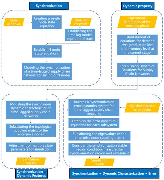
Figure 1.
Supply chain network synchronization model.
Company X’s supply chain network has a total of 72 nodes and its network connectivity diagram is shown in Figure 2.
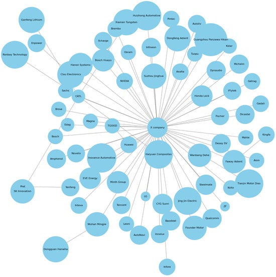
Figure 2.
Company X’s supply chain network connection diagram.
The topological coupling matrix of its network is a sparse matrix, so it is stored in accordance with the Compressed Sparse Row (below), and the storage matrix is as follows:
The column index matrix is as follows:
The row start position index matrix is as follows:
Company T’s supply chain network has a total of 127 nodes and its network connectivity diagram is shown in Figure 3.
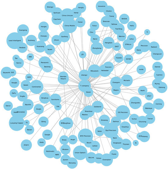
Figure 3.
Company T’s supply chain network connection diagram.
The topological coupling matrix of its network is stored according to Compressed Sparse Row and the storage matrix is as follows:
The column index matrix is as follows:
The row start position index matrix is as follows:
Let the level of demand in the current period be able to be planned based on the linear relationship between the inventory level and the order quantity in the previous period, i.e., , where n denotes the coefficient of outgoing inventory and m denotes the coefficient of order fulfillment. indicates that the level of supply in the previous period was less than the demand of customers’ orders.
The inventory level at the present stage should not only consider the joint influence of demand level and production level, but also the unanticipated losses that may occur, i.e., , where denotes the rate of inventory surplus in the previous stage, and indicates that the inventory in the period is steadily passed on to the period . denotes the coefficient of loss, and indicates that no loss is incurred. b is the intensity coefficient of the joint influence of demand and production.
The level of production in the current period depends on the nonlinear coupling between the inventory level and the firm’s demand level in the previous period as well as the replenishment of the safety stock depletion [20], i.e., , where p denotes the cross-influence intensity coefficient of the demand level and the inventory level; and q denotes the coefficient of the level of the safety stock. denotes the excess of the inventory and the absence of new production.
Based on the above description process, the following mathematical model is constructed:
The rate of change function of the operating parameters is as follows:
The continuous function form of Equation (1) is derived, i.e., the dynamic characteristic model of node i is as follows:
The synchronized dynamic characteristic model considering time lag is as follows:
The complexity of enterprise management stems from the constant change in the internal and external environment [21]. Although each enterprise in the supply chain has its own development concepts and plans, all enterprises focus on the final products or services provided by the supply chain, i.e., the common “attraction”. According to the synchronization model of the time-lagged new energy automotive supply chain network, the dynamic characteristic equations of each enterprise node in the automotive supply chain network are in accordance with Equation (3).
For different parameter settings, the three-dimensional evolution trajectories of the node states are shown in Figure 4.
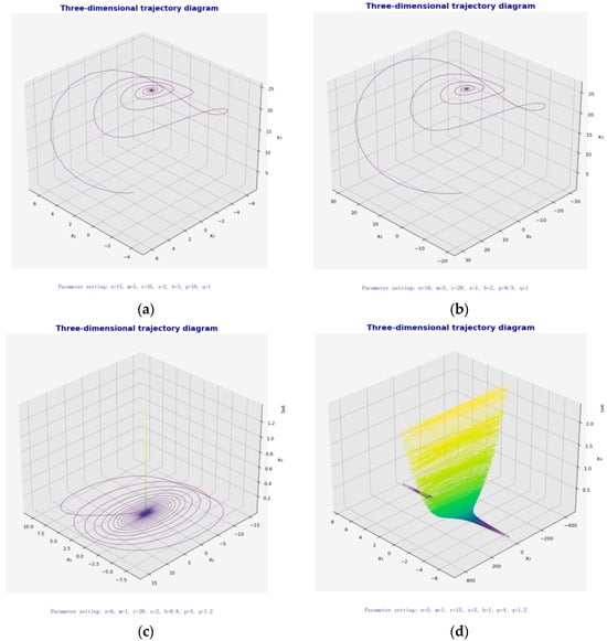
Figure 4.
Three-dimensional evolution trajectory of supply chain node state, (a) Three-dimensional trajectory diagram (n = 15, m = 5, r = 35, s = 2, b = 3, p = 10, q = 1) (b) Three-dimensional trajectory diagram (n = 10, m = 3, r = 28, s = 1, b = 2, p = 8/3, q = 1) (c) Three-dimensional trajectory diagram (n = 6, m = 1, r = 20, s = 2, b = 0.8, p = 4 and q = 1.2) (d) Three-dimensional trajectory diagram (n = 6, m = 1, r = 15, s = 3, b = 1, p = 1 and q = 1.2).
The selection of these parameters is based on the need for system behavior. n and m are positive numbers and n is usually large to reflect the pull of inventory on demand. and should be taken in a range that ensures a reasonable level of inventory, and b and p should be taken to reflect the strength of the joint influence of demand and production. q is usually taken in a small range to indicate that the effect of safety stock on production is weak. We found a combination of parameters that meets the research objectives through several simulation experiments, adjusting the parameter values and observing the dynamic behavior of the system. Overall, the parameters are set based on the characteristics of demand fluctuation, production and inventory management of the actual supply chain to simulate and analyze the system behavior under different scenarios, in order to help study the stability, cyclical fluctuation and loss of control in supply chain management.
The parameter setting of Figure 4a is n = 15, m = 5, r = 35, s = 2, b = 3, p = 10, q = 1, and the parameter setting of Figure 4b is n = 10, m = 3, r = 28, s = 1, b = 2, p = 8/3, q = 1, and the trajectories of the two gradually converge to the stabilized helical attractor, i.e., point attractor, which indicates that the system will always converge to the stabilized state after the change in initial conditions, and exhibits strong stability and low chaos. The point attractor corresponds to the stable equilibrium point of the system, which indicates that the system has a strong self-regulation mechanism under this parameter condition.
In Figure 4c, the parameters are set to n = 6, m = 1, r = 20, s = 2, b = 0.8, p = 4 and q = 1.2, and the system rapidly converges to a periodic trajectory, forming a stable limit ring attractor. The trajectory exhibits periodic oscillations. The limit ring attractor indicates that the system enters a dynamic equilibrium state, which is suitable for describing periodic demand fluctuations in the supply chain, such as seasonal sales behavior.
The parameter setting of Figure 4d is n = 6, m = 1, r = 15, s = 3, b = 1, p = 1 and q = 1.2, and the trajectory is dispersed, which shows the instability of the system, and the system enters into the state of energy explosion, which can be used to explain the system’s out-of-control phenomenon in the case of parameters exceeding the critical value. For example, a vicious circle is triggered by too high or too low inventory in the supply chain. This parameter can be used to study the “critical point behavior” of the system.
In cases where the system exhibits a stable equilibrium (e.g., Figure 4a,b), managers can focus on maintaining stable supply–demand relationships. On the other hand, if the system shows oscillatory behavior (e.g., Figure 4c), businesses may need to adapt to periodic demand variations by implementing seasonal strategies. Finally, for unstable conditions (e.g., Figure 4d), the focus should be on identifying the critical parameters that push the system to an out-of-control state, thus helping prevent catastrophic failures or inefficiencies in supply chain operations.
According to Equation (4), the dynamic characteristics of the new energy vehicle time-lag supply chain network composed of 72 enterprise nodes are modeled as follows:
The synchronization effect of the automotive supply chain network refers to the synchronization of the operations of each enterprise node in the supply chain through coordination and cooperation in order to improve the efficiency of the entire supply chain and its ability to respond to market changes. This synchronization involves a number of aspects such as inventory synergy, matching of production and demand, information sharing, reduction in the bullwhip effect, enhancement of supply chain resilience, optimization of supply chain structure, and promotion of changes in cooperation patterns. Specifically, the synchronization effect implies that firms in the supply chain are able to share information, such as order data, inventory information, and production progress, in order to achieve commonality in inventory management, synergy in production planning, collaboration in purchasing decisions, and coordination in the sales process. In order to make the supply chain network reach synchronization faster, we can add a controller to Equation (5), and let be a solution of network synchronization and when the automotive supply chain network reaches synchronization, the following equation is applicable:
The controller is designed below. We assume that for the differential equation , where and are continuous functions, there exists a unique solution for any initial value and is an m-dimensional vector. And for the vector function , the Lipschitz condition is assumed to hold.
From the definition of global exponential asymptotic synchronization, if the constants exist, where for any initial condition,
then Equation (A6) is said to achieve global exponential asymptotic synchronization. Therefore, the design of the controller is as follows:
which obeys the updated law as follows:
where and are both positive constants. Then, the supply chain network synchronization model is as follows:
The global exponential asymptotic synchronization is reached with the following expression:
Let be a solution of the new energy vehicle supply chain network synchronization model in Equation (10), where . , where is continuous, and . If there exists a non-empty region labelled , , and , the following expression is applicable:
At this point, the supply chain network achieves progressive network synchronization and is a network systematic synchronization region.
The controller designed according to the network in Equation (8) is obtained as , where . In the process of dynamic simulation, we take = 0.1, = 0.1. The model simulation results are shown in Figure 5.

Figure 5.
Simulation of new energy vehicle network synchronization model, (a) Node State Trajectories; (b) Error Convergence Curve.
Figure 5a illustrates the state trajectories of multiple nodes with time , showing obvious periodic oscillation characteristics. The trajectories of different nodes overlap with each other, indicating that the nodes in the network may have strong coupling, and the system reaches a synchronized behavior in a certain time period. In Figure 5b, the red curve indicates the change in the error parameter over time, and the error decreases rapidly at the initial time, suggesting that the control mechanism of the system is able to adjust the node state to be consistent with the reference trajectory quickly. On the other hand, the error curve exhibits oscillatory decay, indicating that the system may have weak damping properties and the system needs some time to fully converge.
According to the simulation results, it can be concluded that in the automotive supply chain network, when the coupling strength between enterprises is kept constant, the increase in the coupling time lag time leads to the growth of the time required for the synchronization process. This indicates that with the extension of the coupling time lag, the information acquired by enterprises at the current stage will lag more, thus making the bullwhip effect in the supply chain more significant. Therefore, one of the effective strategies to reduce the bullwhip effect is to enhance the information exchange between enterprises in the supply chain to ensure that their production plans are consistent with the market demand. In the automotive supply chain network, when the coupling time lag between enterprises is kept constant, an increase in the coupling strength k will shorten the time required for the supply chain network to reach synchronization. This indicates that with the enhancement of the coupling strength, the collaboration between the enterprises in the supply chain is closer, which is conducive to the flow of information in the supply chain, making the production plan more consistent with the actual demand. Therefore, the coupling strength k plays a key role in the synchronization process of the whole supply chain network.
In automotive supply chain management, the establishment of a supply chain network synchronization model has far-reaching theoretical significance and practical application value. The automobile industry is a highly complex, multinational and time-sensitive industry, and its supply chain structure involves a large number of parts suppliers, manufacturers, logistics service providers and sales networks. Each link is not only closely connected in terms of material flow, but also affected by multiple factors such as fluctuations in market demand, changes in raw material prices, policy environment and production capacity. The interaction of these factors can easily lead to the distortion or lag of information transmission in the supply chain, which in turn leads to uncoordination among the nodes of the supply chain, resulting in a series of problems such as the waste of production resources, excess or insufficient inventory, and delivery delays. Therefore, the primary purpose of establishing a supply chain network synchronization model is to eliminate information silos by integrating key information from upstream and downstream links in the supply chain, reduce the negative impact of forecast errors on production planning, and thus realize the coordinated operation of each link in the supply chain. Through this model, enterprises are able to respond to rapid changes in the market, optimize the overall resource allocation, and enhance the flexibility and adaptability of the supply chain through accurate information sharing and instant feedback in a dynamic and open supply chain environment.
3. Measurement of Synchronization Interval of New Energy Vehicle Supply Chain Network
In the process of new energy vehicle supply chain management, the measurement of the synchronization interval of the supply chain network is a crucial issue, especially in the context of the new energy vehicle industry facing rapid technological development, changes in the policy environment, and highly fluctuating market demand. As an emerging industry, the complexity of the supply chain of new energy vehicles far exceeds that of the traditional automotive supply chain, which involves not only core parts and components manufacturers such as batteries, motors, and electronic controls, but also charging facility suppliers, energy management service providers, and policy regulators. Therefore, the links in the new energy vehicle supply chain have high technical dependence and large external uncertainty, and the synchronization requirements between the nodes of the supply chain in production and logistics are more stringent. The measurement of synchronization interval is a kind of quantitative analysis of the coordination and responsiveness between the links in the supply chain, and the accurate measurement can help enterprises better understand the synergistic status of the links in the supply chain, identify possible bottlenecks or information lags, and take corresponding adjustment measures to improve the overall efficiency and resilience of the supply chain.
For the topology coupling matrix of Company X’s network, the eigenvalues −62, −6.84, −3, −2.62, −2.58, −1, −0.42, −0.38, −0.16 and 0 are obtained. Eigenvector is shown in Figure 6 (drawing a feature matrix on a heatmap is a data visualization technique used to show the size or pattern of each element in the matrix through changes in color).
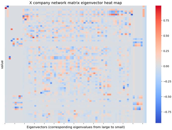
Figure 6.
Eigenvector heat map of Company X’s supply chain network matrix.
Figure 6 shows that the network matrix of firm X is highly sparse, with connections between only a few nodes. This suggests that there are fewer direct relationships between firms in the network and that most firms may rely more on indirect supply chain connections. The network matrix eigenvalues are non-positive, ranging from −62 to close to 0, with only one value of 0 (indicating that the network is weakly connected). The largest negative eigenvalue (−62) indicates that there may be highly centralized nodes (firms) in the network, and the removal of these nodes may significantly affect the stability of the network. Nodes with eigenvalues close to 0 (e.g., −0.16 and 0) correspond to eigenvectors representing nodes such as “Ningde Times”, “Company X”, etc., which may play a key bridging role in the network. A small range of eigenvectors indicates that the network is weakly coupled and the interdependence between nodes is low.
The eigenvalues 0, −0.71, −0.64, −0.49, −0.45, −0.42, −0.18, −0.2, −0.24, −0.31, −0.91, −1.99, −3.73, −7.11, −1.64, −4.3, −4.79, −81.01, −3.71, −3.62, −2.62, −0.38, −1.37, −0.21, −0.29, −1.86, −1.61, −1.0, −3.86, −0.27, −4.82, −3.0, −10.69, −10.92, −8.41, −7.93, −6.79, −2.0, −4.77, −3.85, −2.57 and −1.94 are obtained for the topological coupling matrix of the network of Company T. The eigenvector is shown in Figure 7.
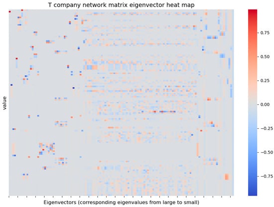
Figure 7.
Eigenvector heat map of Company T’s supply chain network matrix.
Company T’s supply chain network is more complex, with less sparsity and more connections between nodes compared to Company X. This indicates that there are more direct connections between firms in Company T’s network. This suggests that the relationships between firms in Company T’s network are more complex and there are more direct connections. The eigenvalues range from −81.01 to 0, with a wider distribution, where a large negative value (e.g., −81.01) corresponds to a node in the network “Company T”, which is an extremely important node, and its removal may have a significant impact on the network. Eigenvectors with an eigenvalue of 0 indicate that the network has a connected component. Eigenvalues close to 0 (e.g., −0.18 to −0.71) correspond to nodes such as “Company T” and “Changxin Technology”, which may act as bridges or key connectors between important sub-networks in the network. Eigenvectors with large negative eigenvalues, such as “Company T”, “Panasonic”, etc., may reflect the core enterprises in the network, which play a decisive role in the stability of the whole network.
The synchronization condition of the supply chain network system is equivalent to the zero-solution stability condition of the dynamical equations of each error subsystem. With the network topology and node state equations established, the synchronization of the supply chain network mainly depends on the parameters k and . Therefore, the synchronization stability region is determined by the set (k, ). The simplest network is composed of two nodes coupled to each other, and the synchronization stability region is assumed to consist of the set (k, ). According to the synchronization region measurements proposed by Neefs [22] and Oguchi [23,24], the synchronization region coupling strength k based on the number of nodes N = 2 is required for any synchronization region (k, ) with the number of nodes N ≥ 3. Therefore, to estimate the synchronization region of a fully connected network graph with N nodes, we only need to obtain the stable region for the number of nodes N = 2.
The synchronization error vector can be defined as follows:
where . This definition helps us to track the synchronization error of different nodes in the system.
According to the coordinate transformation,
The significance of this matrix transformation is that it transforms into a combination of the state and error of the first node, and as a result, we can more clearly observe the synchronization error between individual nodes. At this point, the dynamical system of the overall supply chain network can be written as follows:
where is the pseudo-inverse matrix of the matrix . and . Equation (15) describes the dynamic system of the entire supply chain network. and denote the time variation of the first node and the synchronization error vector, respectively. and denote the linear dynamics and nonlinear dynamics parts of the system, respectively. is a function that describes the nonlinear coupling. The final time-lag term represents the effect of the state at the previous moment on the current moment, reflecting the time-lag property of the system. According to Equation (15), the synchronization error dynamics of the supply chain network can be obtained as follows:
Equation (16) further develops the dynamic evolution of the synchronization error . It shows how the synchronization error changes over time, i.e., how the speed of the error is driven by the various influences in the system. Diagonalizing its matrix yields an eigenvalue of its matrix with one re-root of and N − 1 re-roots of . Also, since the error vector e(t) is defined by and Equation (13) is composed of N − 1 error subsystems, the error dynamics equations for each of the subsystems can be formulated as follows:
Equation (17) describes the dynamic equations of each error subsystem, which includes the linear part of the system, the nonlinearly coupled part, and the time-lag feedback part. Each error subsystem independently follows a similar dynamic law and interacts with each other through the time lag. For a general supply chain network graph M, where is the eigenvalue of the Laplace matrix , the supply chain network graph M error dynamics equation is as follows:
Consider the simultaneous stable region condition for a fully connected graph of two nodes with an error dynamical system:
where . If the error system described by Equation (5) is asymptotically stable, it implies that the two coupled nodes are asymptotically synchronized.
Let be the region consisting of (, ) that asymptotically stabilizes the error dynamics equation of Equation (18), and then can be estimated using the coupling strength axis based on the synchronization region S of the eigenvalue measure N = 2. Therefore,
Accordingly, to realize the complete synchronization of the automotive supply chain, the coupling strength between enterprises in the network must exceed a certain minimum threshold. When there is a long time lag, the collaborative synchronization of the supply chain network cannot be achieved even if the coupling strength is large, so the synchronization of information exchange between enterprises has a significant impact on the collaborative synchronization of the supply chain. The synchronization stability region of the supply chain network is not only related to the state equations of the nodes, but also related to the coupling strength and time lag between enterprises. Only when the coupling strength exceeds a certain threshold and the time lag of information transfer is small can the supply chain network realize complete synchronization. For a given supply chain network topology, we can use the synchronization stability region determined by the coupling strength and time lag to guide the degree of close collaboration between enterprises and the maximum threshold of time lag. This not only achieves collaborative synchronization among supply chain enterprises, but also achieves collaborative synchronization from an optimal perspective, because strengthening the coupling strength among enterprises and reducing the information time lag require certain costs to maintain. And too close a coupling relationship in addition to high connection costs, to a certain extent, is not conducive to the development of individual enterprises in the supply chain. On the basis of a highly integrated supply chain, enterprises in the supply chain should not only cooperate closely with each other to form strategic alliances, but also maintain relative independence and have the ability to independently manage and deal with emergencies, so as to weaken the negative feedback effect among enterprises in the supply chain. Therefore, in addition to the network space topology of the supply chain, the appropriate coupling strength and time lag are also very important for the collaboration synchronization of the supply chain.
Network synchronization has many impacts on the decision-making of new energy vehicle supply chain, including optimization of production planning and inventory management, logistics distribution and delivery, collaborative supply and risk management, after-sales service and continuous improvement. Through network synchronization, nodal enterprises in the supply chain of new energy vehicles can more accurately predict market demand, so as to formulate reasonable production plans, avoid over-production or under-production, and effectively reduce inventory costs and backlog risks. One can select the optimal distribution route synchronously through the network, improve logistics efficiency, shorten delivery time, and reduce transportation costs. New energy vehicle companies and suppliers can realize real-time information sharing and collaborative work. The two sides can communicate production plans, raw material demand, supply progress and other information in a timely manner, and jointly cope with possible supply disruptions, raw material shortages and other risks. Network synchronization enables the after-sales service of new energy automobile enterprises to receive customers’ fault repair and maintenance requests in real time, and at the same time, adjust after-sales service strategies according to customers’ needs and opinions, provide more personalized services, and enhance customer loyalty.
From the perspective of the actual operation of the new energy vehicle supply chain network, the measurement of the supply chain synchronization interval provides specific improvement directions for enterprises. For example, the supply process of batteries, drive motors and other components may be affected by technological upgrades and policy and regulatory changes, and there is great uncertainty in the production and delivery cycle, and the measurement of the supply chain synchronization interval can help enterprises identify the potential risks in these links, and deploy and optimize the corresponding suppliers and production facilities to ensure the coordination of the supply chain. In practice, enterprises can monitor the production progress, inventory status and logistics distribution of each link in real-time through information technology, so as to accurately assess the synchronization of the supply chain. If the response speed of a link is lagging behind, the enterprise can shorten the synchronization interval by adjusting the production plan, optimizing the inventory strategy or coordinating with the suppliers to improve the response efficiency of the overall supply chain [25]. In addition, the new energy vehicle industry itself has a long industrial chain and a high degree of technological dependence, so not only the manufacturing enterprises themselves, but also the battery manufacturers, charging facility providers, government agencies and other links involved need to work closely together in the supply chain network synchronization model. By measuring the synchronization interval, enterprises can more accurately grasp the production and distribution rhythm of each link, and enhance cross-industry and cross-regional supply chain synergy.
Therefore, the measurement of the synchronization interval of the new energy vehicle supply chain network has important theoretical and practical value. At the theoretical level, this measurement provides a quantitative tool for the precision and intelligence of supply chain management, and promotes the in-depth study of supply chain synergy optimization; at the practical level, it helps enterprises to identify the potential risks and optimization space in the supply chain, and to improve the operational efficiency and resilience of the supply chain through the adjustment of reasonable synchronization intervals, which in turn improves the competitiveness of the enterprises in the dynamic market. With the continuous development of the new energy automobile industry, the synchronization of supply chain will play an increasingly important role in enterprise production, logistics management and risk control, and become one of the key factors for enterprises to maintain their leading position in the market.
4. New Energy Vehicle Supply Chain Network Synchronization Optimization Strategies and Suggestions
In the process of collaboration and synchronization optimization of the new energy vehicle supply chain network, the coupling matrix L, the coupling strength k between enterprises, and the time lag τ of information exchange between enterprises are the key factors affecting the synchronization ability of supply chain. By optimizing the topology and network parameters of the supply chain network, the synchronization and collaboration ability of the supply chain network can be effectively improved.
4.1. Optimization Strategies
Based on the mathematical model and the main network parameters of Company X and Company T, it is easy to see that the number of nodes and edges of Company T is significantly larger than that of Company X, which indicates that the supply chain network of Company T is more complex, and the collaboration and management of the enterprise nodes are relatively more difficult; while Company X, which has fewer nodes, may have a more concise network structure and a lower complexity of collaboration, but there may be a lack of information flow. The average path length of Company T is larger than that of Company X, which indicates that there may be greater delays in information flow and less efficient collaboration among nodes, while the shorter average path length indicates that Company X has a more compact network structure and faster information transfer. However, too short paths may lead to overdependence on core nodes, exposing them to greater loads and risks. Therefore, a better path length should strike a balance between information flow efficiency and network robustness. The clustering coefficient of Company T is slightly higher than that of Company X, which indicates that the collaboration between the enterprise nodes in its network is closer, and it has a stronger ability to share resources and exchange technology; while a lower clustering coefficient may imply that Company X’s network has poorer local connectivity and less efficient cooperation, but it may also make it have higher flexibility and decentralization characteristics. The number of eigenvalues of Company T is significantly higher than that of Company X, which indicates that its supply chain network has higher complexity and higher coordination costs, while the fewer eigenvalues of Company X may imply that its network is more likely to reach a synchronized state and has higher collaboration stability.
From this, we can derive the following optimization schemes:
4.1.1. Optimize the Network Structure
The network coupling matrix L is one of the core elements of the supply chain network, reflecting the supply–demand cooperative relationship between the enterprises in the supply chain. The topology of the network directly determines the collaboration efficiency and synchronization ability of the supply chain. According to the complex network theory “structure determines function”, different network structures have different synchronization characteristics and dynamic characteristics of behavior; therefore, by optimizing the network structure, the supply chain collaboration ability can be fundamentally improved. Specific strategies include the following points.
First, one can reduce the average distance of the network and improve the clustering coefficient. The shorter the average distance of the network, the faster the information circulation and the more rapid the system response. At the same time, a higher clustering coefficient means that the nodes in the network are more closely connected to each other and the information dissemination is more efficient. In supply chain networks, the synchronization ability and information flow efficiency of the supply chain can be significantly improved by adjusting the connection method, shortening the average path length in the network and increasing the clustering coefficient between nodes. While maintaining the growth of the supply chain topology, the node connection scheme is preferred, and the clustering characteristics of the network are used to optimize the relationship between the nodes to ensure the high efficiency and low time lag of information exchange.
Second, one can optimize the eigenvalues of the node connection and coupling matrix. During the evolution of the supply chain network, the synchronization ability of the network will gradually decrease with the addition of new enterprises [26]. In order to maintain the synchronization performance of the network, the optimal connection should be preferred when new enterprises join the network, i.e., to ensure that the cooperative relationship established between the newly joined enterprises and the existing enterprises in the supply chain can minimize the loss of synchronization performance of the system. This can be achieved by adjusting the second-largest eigenvalue of the coupling matrix L. When selecting new enterprises to establish cooperation with existing enterprises, priority is given to reducing the second-largest eigenvalue of the coupling matrix so as to enhance the synchronization of the supply chain as a whole.
Third, one can reduce the load of key nodes by reducing the maximum meson number. Excessive loads of key nodes in the supply chain may lead to a decrease in the synchronization efficiency of the system, especially in unexpected events, and the overload of key nodes may become a bottleneck and affect the operation of the whole network. Therefore, reducing the load of key nodes and lowering the maximum number of mediators in the network are important measures to optimize the synchronization of supply chain networks. By optimizing the node connections in the network, the load of key nodes is reasonably distributed to avoid the key nodes from becoming a single point of failure, so as to guarantee the stability and efficiency of the supply chain [27]. Specifically, the following two optimization methods are given in this paper.
- Method 1: Adding connectivity edges to less connected or overloaded nodes
Optimization is carried out by optimizing nodes with low connectivity (degree < 3) with overloaded nodes with high connectivity (degree > 5) in order to reduce bottlenecks in the network. The constraint is that the two nodes must be currently unconnected to each other. The average path length of the corresponding network structure of Company X is 2.23, and the clustering coefficient is 0.06. The most heavily loaded node is “Company X”, which is “SK Korea”. The most heavily loaded node is “Company X”, which connects “SK Korea”, “Ningbo Rongbai”, “Changyuan Shenrui”, “Amphenol”, “Qunchuang” and “Company X”. “Company X”, “SK Korea”, “Ganfeng Lithium”, “Haiyuan Composites”, etc., are connected with “Ningde Times”. The average path length of the new network structure is 1.94, and the clustering coefficient is 0.97. The optimized network structure of Company X that corresponds to the network connection diagram is shown in Figure 8.
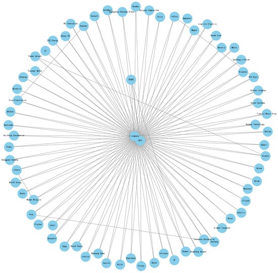
Figure 8.
Diagram of the supply chain network optimization structure of Company X in Optimization Method 1.
The topological coupling matrix of its network is stored according to the Compressed Sparse Row and the storage matrix is as follows:
The column index matrix is as follows:
The row start position index matrix is as follows:
For the optimized topological coupling matrix of Company X’s network, the eigenvalues −72, −4, −2 and 0 are obtained and the eigenvectors are shown in Figure 9.
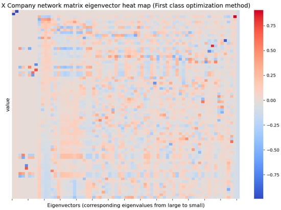
Figure 9.
Optimized Company X supply chain network matrix eigenvector heat map in Optimization Method 1.
The average path length of the corresponding network structure of Company T is 2.67, and the clustering coefficient is 0.08. The bottlenecks in the network are reduced by optimizing the nodes with low connectivity or the nodes with high connectivity but heavy loads. The most heavily loaded nodes are “Company T”, “Changxin Technology” and “Hengdian Dongmag”, while the least connected nodes are “Minmetals Capital”, “Pioneer Capital”, “Pioneer Capital”, and “Hengdian Dongmag”. The nodes with the lowest connectivity are “Minmetals Capital”, “Pilot Intelligence” and “Luoyang Copper”. “Minmetals Capital”, “Pilot Intelligence”, “Ganfeng Lithium”, “Luoyang Copper”, “Grimme”, “China Baoan”, etc., are connected to “T-companies” and “Sanshan shares”. “Hebei Xuan Gong”, “Wada Industry”, etc., are connected to “Changxin Technology” and “Hitachi Chemical” and “Huden” to “Huden”. The average path length of the new network structure is 1.90, and the clustering coefficient is 0.28. The optimized network structure of Company T is shown in Figure 10.
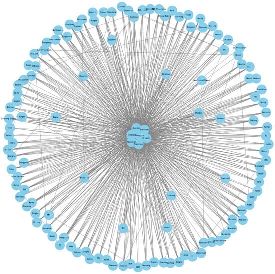
Figure 10.
Diagram of the supply chain network optimization structure of Company T in Optimization Method 1.
The topological coupling matrix of its network is stored according to the Compressed Sparse Row, and the storage matrix and column index matrix are as follows, respectively:
The row start position index matrix is as follows:
For the optimized topological coupling matrix of Company T’s network, the eigenvalues are −126.06, −113.68, −110.40, −105.87, −9.34, −9.00, −8.64, −8.25, −8.00, −7.00, −3.35, −3.00, −2.68, −2.52 and 0, and the eigenvector is shown in Figure 11.
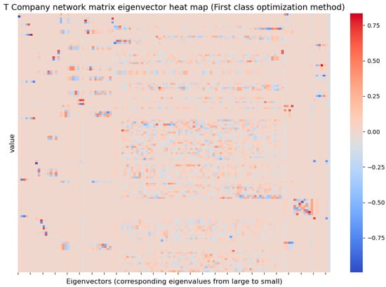
Figure 11.
Optimized Company T supply chain network matrix eigenvector heat map in Optimization Method 1.
The main parameters of the networks of Company X and Company T before and after optimization are shown in Table 2. The number of nodes and the number of edges reflect the scale and complexity of the supply chain network, the average path length can reveal the coordination efficiency of the supply chain, the clustering coefficient reflects the closeness and cooperation density of the local nodes in the supply chain network, and the number of eigenvalues reflects the network synchronization.
Table 2.
Comparison of the main parameters of Company X and Company T’s networks in Optimization Method 1.
By optimizing the nodes with low connectivity or nodes with high connectivity but heavy loads in the networks of Company X and Company T, i.e., increasing the number of edges of the nodes with low connectivity or nodes with heavy loads in the networks, the overall performance of the networks is improved. In the optimization of Company X, the addition of new edges further strengthens the influence of bridge nodes such as “Company X” and “Ningde Times”, making their role in the whole network more prominent. After optimization, the number of edges of Company X increases from 73 to 148, the average path length decreases from 2.23 to 1.94, the clustering coefficient increases from 0.06 to 0.97, and the number of eigenvalues decreases from 8 to 4. Similarly, in the optimization of Company T, the newly added edges further strengthen “Company T”, “Changxin Technology” and “Hengdian Dongmag”, etc. After optimization, the number of edges of Company T increases from 154 to 786, the average path length decreases from 2.67 to 1.90, the clustering coefficient increases from 0.08 to 0.28, and the number of eigenvalues decreases from 42 to 16. In addition, the number of eigenvalues decreases from 42 to 16.
After optimization, the number of edges of the two companies increases, which means that more cooperative relationships are added between the nodes of the companies in the supply chain network, and the connection density of the network increases significantly. The added connected edges make the local coupling degree of the network significantly stronger [28], and the control ability of the high centrality nodes in the network to the surrounding nodes increases. Such changes indicate that the optimization process may have introduced more information sharing and collaborative mechanisms, which enhances the network’s collaborative ability and reduces the problems of information silos and unequal distribution of resources.
The decrease in the average path length of the two companies indicates that the intermediate steps required to reach from one node to another in the network have been reduced, and the transmission speed of information and resources has been significantly increased, and the overall efficiency of the supply chain has thus been strengthened, enabling it to respond more quickly to changes in the market demand and the environment, and to reduce the risks caused by delays in the transmission of information.
The increase in the clustering coefficient of the two companies indicates that the local connection between enterprises in the network is closer, and the collaborative relationship between enterprises is stronger. This network structure helps the information and technology sharing between enterprises, especially in complex decision-making and joint innovation, showing higher efficiency, and also improves the network’s risk-resistant ability, making the supply chain more resilient.
The reduction in the number of eigenvalues of the two companies indicates that the redundancy of the network is reduced, the structure is more centralized and efficient, the synchronization performance of the network is improved, and the difficulty of collaborative operation is reduced, and it also indicates that the network is more likely to reach a stable state of synergy, so that the optimization of the network can reduce the complexity of the supply chain management and improve the efficiency of the overall coordination.
During the optimization process, because the original network size of Company T is larger, it pays more attention to improving the connectivity and collaboration ability of the network by adding a large number of new edge connections in the optimization process, which leads to the growth of the number of edges and the final number of edges of Company T to be significantly higher than that of Company X. The company prefers to keep the network moderately connected, and the newly added edges are mainly concentrated between key nodes, focusing on precise optimization rather than large-scale connection increase.
Moreover, due to the high path length and low information flow efficiency of Company T, the path length is effectively shortened by adding a large number of new edges. In contrast, the original path length of Company X is already relatively short, so there is less room to shorten the path after optimization. Although the optimized path lengths of the two companies are very close to each other, indicating that both companies achieve high information flow efficiency and fast response capability after optimization, the optimization of Company T is larger.
Company X exhibits a high degree of clustering after optimization, indicating that the local cooperative relationship between enterprises in its supply chain network is extremely close, which helps to strengthen information sharing, resource complementation and technology synergy. The clustering coefficient of Company T, although also improved, is still much lower than that of Company X. This reflects that Company T pays more attention to the enhancement of global connectivity in the optimization process and pays insufficient attention to the close collaborative relationships of local nodes. Company T prefers to enhance efficiency through the improvement of connectivity in the overall network rather than the enhancement of local collaboration.
The absolute value of the number of eigenvalues of Company X is much smaller than that of Company T, indicating that the supply chain network of Company X tends to be more simplified and synchronized after optimization, and the overall collaboration difficulty is lower, which shows higher synchronization performance. Although the number of eigenvalues of Company T decreases significantly, due to the large number of nodes in Company T, the absolute value is still higher, which indicates that the network is still of high complexity and synchronization difficulty, and may need further optimization to improve collaboration efficiency.
In supply chain network optimization, targeted optimization strategies should be formulated according to the specific needs of enterprises and network characteristics. Taking Company X and Company T in this paper as an example, due to the differences in the scale, characteristics and optimization goals of the supply chain networks of the two companies, Company X pays more attention to improving the synchronization ability and local collaboration efficiency of the network through accurate local optimization and high clustering coefficient, and its network shows close and highly collaborative characteristics, while Company T tends to increase the global connectivity significantly to enhance the overall connectivity and fast response ability of the network, but the network scale itself is very large, and it is very complex and difficult to improve collaboration. Given its fast response capability, but large network size, the enhancement of local collaboration is relatively limited, and the degree of improvement in network synchronization is not as significant as that of Company X. In terms of practical application, Company X’s optimization strategy may be more suitable for scenarios that require high collaboration efficiency and close local cooperation, while Company T’s optimization strategy is more suitable for supply chain environments that are large in scale and need to respond quickly to market demands.
- 2.
- Method 2: Adding connecting edges between nodes with long path lengths
Adding connecting edges to pairs of nodes with long path lengths reduces the average path length of the network. First, find out all the node pairs that are not directly connected and calculate the shortest path length of these node pairs. Second, sort the node pairs in descending order of path length and prioritize adding edges for the node pairs with the longest paths. Limit the number of added edges to 100 to avoid over-modifying the network structure. After the final addition of edges, the network characteristics are recalculated.
The average path length of the corresponding network structure of Company X is 2.23, and the clustering coefficient is 0.06. The average path length of the network structure of Company X is 2.23, and the clustering coefficient is 0.06. The average path length of the corresponding network structure of Company X is 2.23, and the clustering coefficient is 0.06. The “SK Korea”, “Ganfeng Lithium”, “Ningbo Rongbai” and so on are connected to “Infineon” and “Inconel”; “Dongguan Hanwha”, “Goldfarb” and so on are connected to “Pritchard”, “Pratt”, “Haiyuan Composites”, “Dongguan Hanwha”, “Encore” and “Xiamen Tungsten”. The average path length of the new network structure is 2.11, and the clustering coefficient is 0.16. The optimized network structure of Company X is shown in Figure 12.
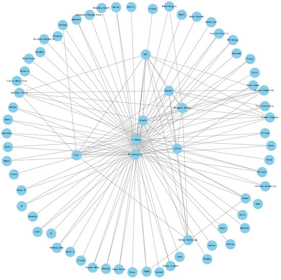
Figure 12.
Diagram of the supply chain network optimization structure of Company X in Optimization Method 2.
The topological coupling matrix of its network is stored according to the Compressed Sparse Row and the storage matrix is as follows:
The column index matrix is as follows:
The row start position index matrix is as follows:
The eigenvalues are −61.02, −32.04, −12.11, −10.83, −6.00, −4.00, −2.98, −2.00, −1.26, −1.00, −0.68 and 0, and the eigenvector is obtained for the optimized topology coupling matrix for Company X’s network as shown in Figure 13.
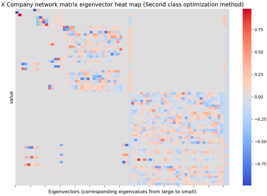
Figure 13.
Optimized Company X supply chain network matrix eigenvector heat map in Optimization Method 2.
The average path length of the corresponding network structure of Company T is 2.67, and the clustering coefficient is 0.08. The nodes with longer paths are optimized by adding edges to reduce bottlenecks in the network. The nodes of “Sugo”, “Luoyang Copper”, “Coldray Cobalt” and “Greenpeace” are clustered with the nodes of “Minmetals Capital” and the nodes of “Cobalt” and “Greenpeace” are clustered with the nodes of “Cobalt” and “Greenpeace”. Nodes such as “Minmetals Capital” are connected to nodes such as “China Bao’an”, “Tianqi Lithium” and “YWL”. Nodes are connected to “Pilot Intelligence” and “Nanyang Science and Technology”, “Xinzhoubang” and “Changyuan Group”. The average path length of the new network structure is 2.41, and the clustering coefficient is 0.08. The optimized network structure of Company T corresponds to the network connectivity diagram shown in Figure 14.
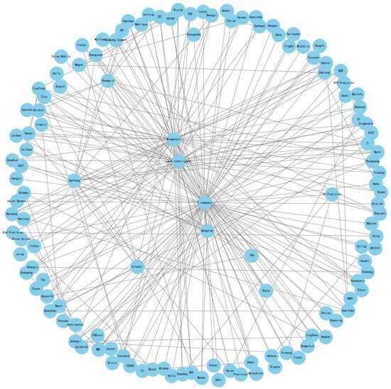
Figure 14.
Diagram of the supply chain network optimization structure of Company T in Optimization Method 2.
The topological coupling matrix of its network is stored according to the Compressed Sparse Row, and the storage matrix and column index matrix are as follows, respectively:
The row start position index matrix is as follows:
The eigenvalues are −81.01, −46.09, −12.11, −44.00, −17.19, −11.08, −7.63, −5.61, −4.80, −4.34, −3.93, −3.62, −3.39, −3.00, −2.74, −2.24, −1.98, −1.70, −1.38, −1.00, −0.45 and 0 and the eigenvector is shown in Figure 15.
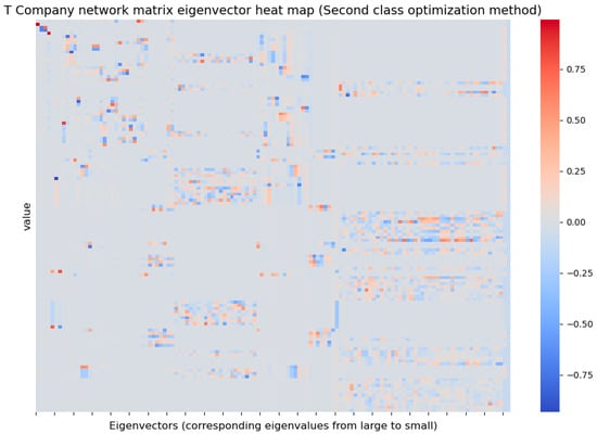
Figure 15.
Optimized Company T supply chain network matrix eigenvector heat map in Optimization Method 2.
The key parameter pairs of Company X and Company T networks in Optimization Method 2 are shown in Table 3. By optimizing the node pairs with longer paths in the network of Company X and Company T, the path lengths between the key nodes in the network are reduced so as to improve the efficiency of information flow and the transfer speed of resources. After optimization, the number of edges of company X increases from 73 to 148, the average path length decreases from 2.23 to 2.11 and the clustering coefficient increases from 0.06 to 0.16, but the number of eigenvalues increases from 8 to 12. After optimization, the number of edges of Company T increases from 154 to 786, the average path length decreases from 2.67 to 2.41, the clustering coefficient remains unchanged, and the number of eigenvalues decreases from 42 to 22.
Table 3.
Comparison of the main parameters of Company X and Company T’s networks in Optimization Method 2.
Similar to Method 1, in Method 2, the number of edges increases, the average path length decreases, the clustering coefficient of Company X increases, and the number of eigenvalues of Company T decreases after optimization in Company X and Company T. All of these indicate that the two companies have improved the overall collaborative efficiency and synchronization capability of the supply chain network through optimization, so that the supply chain network has a higher degree of flexibility, stability, and responsiveness after optimization.
However, the number of eigenvalues of Company X rises from 8 to 12, reflecting the increase in network complexity and the change in dynamic characteristic behavior brought about by the addition of new connected edges. During the optimization process, the distribution of edges and the increase in local connectivity create more local “subgroups” or dynamic patterns, which may lead to an increase in the difficulty of global synchronization and coordination while enhancing local collaboration. In addition, the increase in the number of eigenvalues also stems from the different focuses of the optimization objectives. This optimization mainly focuses on improving network connectivity and local collaboration, while the change in the eigenvalues is not a direct optimization objective, so the increase may be a by-product of the optimization process of other indicators. Although the increase in the number of eigenvalues reflects the complexity of synchronization to some extent, it does not diminish the improvement of overall network collaboration efficiency. The optimization results show the control of the trade-off relationship between local collaboration and global synchronization, while providing direction for further improvement of synchronization performance in the following.
Meanwhile, the clustering coefficient of Company T remains unchanged, which is closely related to the distribution mode of the newly added connecting edges. In the supply chain network optimization process, the change in the clustering coefficient mainly depends on whether the newly added edges are concentrated among local nodes to form a tighter triangular structure. In Optimization Method 2, Company T’s optimization strategy favors the increase in global connectivity, i.e., the newly added edges span more distances between different regions or groups of nodes to improve the connectivity and information flow efficiency of the overall network rather than to enhance the clustering of local nodes. Although this optimization improves the global collaboration ability and response speed of the network, it has not significantly affected the local connection density, so the clustering coefficient remains unchanged. This result reflects the difference in the orientation of the optimization objectives, focusing on shortening the average path length and reducing the global dynamic complexity, without prioritizing the adjustment of the local nodes’ collaboration tightness, which leads to no change in the clustering coefficients.
Both Method 1 and Method 2 reflect the same optimization objectives and characteristics in optimizing the supply chain network by increasing the connecting edges to improve the network structure, thus enhancing the overall performance of the supply chain. Both methods significantly increase the number of edges in the network and reduce the average path length, indicating that both methods enhance the information flow and resource transfer efficiency between nodes to different degrees, and both methods have an impact on the local and global characteristics of the network. Despite the different focuses of optimization, both of them show positive effects on the connectivity and dynamic behavior of supply chain networks by adjusting the network topology, indicating that they have consistent underlying logic and technical paths in optimizing network performance.
Method 1 aims to balance the load distribution and resource sharing of nodes in the network by establishing connecting edges between nodes with lower connectivity and nodes with higher loads, which significantly improves the local aggregation and the overall synergistic efficiency of the network. This optimization approach increases the clustering coefficients of both Company X and Company T by a large margin (from 0.06 to 0.97 for Company X, and from 0.08 to 0.28 for Company T), and at the same time effectively reduces the number of eigenvalues, reflecting the reduction in network complexity and synchronization difficulty. In contrast, Method 2 emphasizes the optimization of global connectivity and the improvement of information flow efficiency mainly by adding connecting edges between nodes with longer paths to shorten the average path length of the network. Since this method focuses more on global path adjustment than local collaboration enhancement, its improvement in clustering coefficients is more limited (from 0.06 to 0.16 for Company X, and the clustering coefficients are unchanged for Company T), and even triggers a rise in the number of eigenvalues in Company X, indicating that synchronization of the network has become more difficult. This difference shows the different orientations of the two methods in terms of optimization objectives and strategies: method 1 focuses on local collaboration and load balancing, which is suitable for enhancing the stability and robustness of the network; while method 2 is biased towards the optimization of global information flow, which is more suitable for enhancing the response speed and overall efficiency of the supply chain.
Based on the qualitative and quantitative analysis of Optimization Method 1 and Optimization Method 2, it is easy to see that the specific effect of supply chain network optimization depends largely on the setting of optimization objectives and the selection of optimization methods, and different strategies have their own advantages and disadvantages in strengthening local or global performance. Therefore, supply chain network optimization needs to seek a balance between local optimization and global optimization according to the characteristics of the network and the needs of enterprise objectives. Focusing only on local collaboration may lead to insufficient global efficiency, while focusing only on global connectivity may neglect local stability and risk resistance. The combined use of the two methods, or the selection of appropriate optimization strategies according to different scenarios, can help supply chain managers to improve overall efficiency while taking into account the stability and complexity control of the network, and ultimately achieve the organic combination of efficient supply chain operation and risk prevention and control. This goal-oriented optimization strategy selection provides a practical reference for the design and improvement of supply chain networks.
For enterprises, increasing the connecting edges in the network corresponds to the establishment of inter-enterprise cooperative relationships in reality. More direct connections between suppliers, manufacturers, distributors, etc., are established through electronic data exchange, information sharing platforms, and cooperation agreements to ensure that enterprises in different segments of the supply chain can exchange information, resources, and demands more efficiently, accurately transmit inventory, production progress, and demand changes to avoid information lags and errors, and be able to realize more rapid information flow and resource sharing, avoid information silos or collaboration bottleneck, optimize resource allocation, directly reduce ineffective communication and duplication of work and improve the overall efficiency of resource use, which in turn reduces operating costs and improves productivity. It also helps enterprises reduce the intermediate links of information transmission in the supply chain and shorten the path of information flow, which helps accelerate the decision-making process and enables enterprises to respond to market changes and customer needs in a shorter period of time. In response to emergencies or market fluctuations, even if a supplier has problems, the enterprise can quickly adjust the source of supply through the established additional cooperative relationship, reducing the dependence on a single supplier or partner. The nodes in the supply chain support and complement each other, improving the overall ability to adapt to external changes and avoiding the risks associated with supply chain disruptions.
4.1.2. Optimizing the Coupling Strength k and Time Lag
Coupling strength k and information time lag t are the key parameters of the edges in supply chain networks, which directly affect the efficiency of collaboration between enterprises and the speed of information transmission. Increasing the coupling strength k can enhance the close collaboration between enterprises and is conducive to the rapid dissemination and feedback of information, but too high a coupling strength may also lead to excessive dependence on the supply chain and reduce the independence of enterprises. The time lag t is the time required for information to be transmitted in the network, and too long a time lag reduces the efficiency of information exchange, so optimizing the coupling strength and time lag is the key to improving the synchronization capability of the supply chain. Specific strategies include the following:
- Moderately increasing the coupling strength
Increasing the coupling strength can enhance collaboration and information sharing among enterprises in the supply chain and accelerate the decision-making and feedback process. However, too high a coupling strength may increase operational costs and lead to rapid loss of control of the entire supply chain when unexpected events occur. Therefore, the coupling strength should be kept at a moderate level to balance the cost and collaboration efficiency. While enhancing the coupling strength, it is necessary to consider the balance between cost and benefit to avoid the over-dependence and risk brought by too high coupling strength. The optimal coupling strength can be found by simulating the network behavior under different coupling strengths.
In practice, optimizing the coupling strength means adjusting the degree of cooperation and the frequency of information exchange among enterprises in the supply chain to achieve the best collaboration efficiency. By signing clear cooperation agreements with partners, enterprises can set reasonable delivery times, production schedules and inventory levels to optimize the coupling strength. Optimizing coupling strength can lead to more efficient collaboration between different parts of the supply chain. For example, by increasing the frequency of cooperation between suppliers and manufacturers to ensure more accurate information transfer and more timely inventory management, enterprises can ensure that each link in the supply chain can respond more quickly to changes in market demand by sharing data such as sales forecasts, production schedules and inventory levels.
- 2.
- Reduce the time lag of information transfer
The time lag of information transfer t affects the speed of feedback and the efficiency of decision-making among enterprises. A short time lag can improve the speed of information flow and enhance the responsiveness of the supply chain. However, the shorter the information time lag, the better, because under the existing information technology conditions, the length of the time lag is limited by the network architecture and the level of technological development. By introducing advanced information technology, unnecessary time lag can be reduced and the speed and accuracy of information transmission can be improved. At the same time, the speed of information transmission and the reliability of information should be balanced to avoid information errors caused by too frequent updating of information.
In practice, optimizing the time lag refers to improving the real-time and accuracy of decision-making by reducing the delay in the information transmission process. Using big data analysis and artificial intelligence algorithms, enterprises can achieve more accurate demand forecasting and production scheduling, reducing the decision-making delay caused by time lag. Optimizing time lag can reduce the response time of decision-making by accelerating information transfer. Enterprises can obtain important information such as sales data, inventory status and production progress in real-time, so that they can make adjustments more quickly and avoid production interruptions or resource wastage due to information lag. For the fast-changing market, optimizing the time lag is especially important, which can help enterprises seize market opportunities, adjust the inventory quantity and supply chain scheduling in a timely manner, reduce the inventory cost and improve the utilization rate of resources, and avoid the backlog of inventory or supply chain rupture.
- 3.
- Appropriately reduce the impact of time lag on enterprise independence
The time lag in the supply chain not only affects the speed of information transmission, but also may affect the independence of enterprises. When the time lag is too long, the information transfer is not timely, which may lead to excessive interference of the enterprise’s strategic decisions by external information, which is not conducive to the enterprise’s autonomy and production arrangements. The application of information technology should be improved to reduce the time lag in information feedback between enterprises, while avoiding excessive reliance on external information, thus maintaining the strategic independence of enterprises.
Enterprises can implement enterprise resource planning (ERP) systems, supply chain management (SCM) systems or advanced Internet of Things (IoT) technology to realize information sharing and real-time data updating in each link of the supply chain, reduce the impact of time lag on enterprise independence, and promote close cooperation and rapid response among enterprises.
4.1.3. Optimize the Degree of Collaboration
The appropriate degree of collaboration between enterprises is crucial to the coordinated development of the supply chain. The appropriate degree of collaboration can not only reduce the management difficulty, but also enable enterprises to play their respective advantages in the supply chain to avoid excessive centralization and dependence. The appropriate intensity of collaboration can promote the formation of synergies among the parties in the supply chain, while avoiding over-dependence and maintaining the independence and autonomous decision-making ability of enterprises. By constructing a flexible cooperation mode and maintaining moderate collaboration among enterprises in the supply chain, the transmission of information and material flows can be made more efficient.
By guiding the actual operation through the optimization methods proposed in this section, enterprises can significantly improve the quality and accuracy of decision-making, effectively reduce the complexity of supply chain management, not only improve short-term operational efficiency and customer service level, but also enhance the market adaptability in the long-term strategic level, promote innovation, achieve sustainable development, and ultimately maintain a competitive advantage in the complex market environment.
4.2. Policy Recommendations
Based on the analysis of the synchronous optimization of the automotive supply chain network, the following policy recommendations can be put forward, aiming to enhance the overall collaboration and risk-resistant capability of the supply chain through optimizing the topology of the network, strengthening network collaboration, promoting innovation, and improving the transparency of information, so as to further promote the sustainable development of the automotive industry [29].
Firstly, from the perspective of systematization, the topology of the automotive supply chain network should be developed in the direction of small world, scale-free and decentralization. The automotive supply chain presents heterogeneous network characteristics, which means that nodes with smaller degree values tend to be connected with nodes with larger degree values, while most enterprise nodes have lower degree values. In order to enhance the collaborative synchronization ability of the supply chain and reduce the probability of network risk propagation, the “decentralization” strategy should be implemented moderately while maintaining the scale-free characteristics of the network. This strategy helps to reduce the load of core nodes, improve the robustness of the network, and enhance the network’s ability to defend against external shocks and malicious attacks. Through decentralization, members of the supply chain can establish a more equal partnership, which not only enhances the efficiency of inter-enterprise collaboration, but also improves the overall synchronization ability of the network. In addition, decentralization can also enhance the network’s stress resistance, so that the failure of individual enterprise nodes will not have an excessive impact on the operation of the whole supply chain.
On the other hand, the scale-free network characteristic of the automotive supply chain requires us to focus on the cultivation and management of “convergence nodes”. In the supply chain network, key nodes such as core manufacturing enterprises usually play a crucial role. As the core of the industry chain, vehicle manufacturers not only play a leading role in digesting excess capacity and promoting industrial optimization and restructuring, but also have a decisive influence in promoting regionalized supply-side reform and maintaining competitive advantages. Therefore, it is suggested that through the network nesting feature, the core enterprises should take the initiative to take the lead in promoting resource integration and complementary advantages with other key enterprises in the supply chain to further enhance the collaborative synchronization capability of the whole supply chain. Through this kind of in-depth cross-enterprise cooperation, the supply chain can be more flexible and responsive in the face of market changes, and bring rapid growth and development for the regional economy.
From the national policy level, the automobile industry should be encouraged to form a regional cluster development mode oriented by brand, so as to promote the overall structure of the supply chain towards the development of “small world” characteristics. A small world network has shorter average path lengths and higher clustering coefficients, which makes the information spread more efficiently in the network, and is conducive to the rapid realization of technology and resource sharing among enterprises. Through the development of regional clusters, it can not only improve the efficiency of information circulation, but also promote collaboration among supply chain members, thus enhancing the synchronization ability of the whole supply chain and ensuring its stable operation. In addition, the economies of scale formed by regional clusters will further promote the refinement of the division of labor within the supply chain, prompting the continuous optimization and upgrading of the industrial structure, and helping the automotive industry to move towards a more advanced stage of development.
At the same time, with the increasing complexity and dynamics of the automotive supply chain, all enterprises should undertake social responsibility and promote the coordinated development of the supply chain. Technological innovation plays a crucial role in this process, which can effectively enhance the overall operational efficiency and responsiveness of the supply chain [30]. Therefore, it is recommended that the government and industry authorities increase their support for technological innovation, especially technological breakthroughs in the fields of smart manufacturing, big data application and artificial intelligence, to further promote the digital transformation of the supply chain [31]. In addition, the establishment of a fair and reasonable benefit distribution mechanism to ensure that all enterprises realize win–win sharing in cooperation is also the key to promoting the healthy development of the supply chain. By creating a healthy ecosystem, it can not only improve the overall effectiveness of the supply chain, but also enhance the stability and resilience of each link in the industry chain.
From the micro level, each enterprise node in the supply chain should adopt different development strategies according to its position in the network in order to improve its role and influence in the supply chain. For the “convergence nodes” in the automotive supply chain (i.e., core enterprises and their important partners), it is necessary to firstly strengthen the protection measures to prevent the normal operation of the supply chain from being affected by malicious attacks or other external risks. In order to ensure the security of the supply chain, it is recommended to increase redundant connections, divest the non-core business of core enterprises, reduce their monopoly in the supply chain, and promote the decentralization of the network. Core enterprises should give full play to their leadership role, promote equal cooperation among enterprises, supervise each other and develop together, so as to improve the overall synchronization and coordination ability of the supply chain. In addition, core enterprises should consolidate their management position in the supply chain through technological innovation, and at the same time integrate more advantageous resources and services to promote the transformation and upgrading of the automotive industry.
As for the “non-critical node” enterprises, they should firstly improve their innovation ability and market competitiveness, and enhance their position in the supply chain by providing core technology, high-quality services or scarce resources. These enterprises should take advantage of their own strengths to establish strategic cooperative relationships with other enterprises in the supply chain, forming cooperative alliances for resource sharing and technology sharing, and maximizing benefits through “strong alliances”. Through this kind of cooperation, non-critical node enterprises can not only improve their innovation ability, but also expand their market share and enhance their influence in the supply chain. More importantly, non-key node enterprises should consider the optimization of geographic location, as close as possible to the core enterprises or other key nodes, which is conducive to industrial agglomeration and the formation of economies of scale, but also with the technology and resources of the core enterprises to continue to enhance their competitiveness.
In the dynamic development process of the automotive supply chain, all enterprises in the supply chain should have the right to independently choose to join or leave the network. To this end, the key enterprise nodes in the network should play a leading role in leading other enterprises in the supply chain to expand their scale, enhance their reputation and continuously improve their innovation ability. At the same time, the development of a reasonable benefit distribution model and responsibility mechanism will help attract more advantageous enterprises to join the supply chain and further enhance the competitiveness and market responsiveness of the supply chain [32].
Finally, with the continuous refinement of the social division of labor, the expansion of enterprises in the automotive supply chain may trigger the “bullwhip effect”. Therefore, information sharing should be one of the effective strategies to mitigate the bullwhip effect. Enterprises should adopt new technologies to improve information transfer efficiency and establish a more transparent information sharing platform. Suppliers can cooperate to form supplier alliances to reduce unnecessary inventory and improve information transparency; at the same time, sellers should keep in touch with key supplier nodes as much as possible when feeding back demand information to core enterprises to reduce inventory fluctuations in the supply chain.
5. Conclusions
In conclusion, this study provides critical managerial insights into the challenges and opportunities surrounding supply chain information synergy in the context of new energy vehicles under intelligent manufacturing. The findings reveal that information quality—encompassing standardization, security, completeness, and flexibility—plays a pivotal role in enhancing supply chain information synergy and, consequently, supply chain performance. Managers should prioritize improving these dimensions of information quality across supply chain nodes to foster greater collaboration and operational efficiency. Additionally, this study highlights the importance of information synergy efficiency as a direct driver of supply chain performance, underscoring the need for streamlined processes and technological integration.
From a nobility perspective, network synchronization optimized supply chain node enterprises can more accurately demand forecast and inventory management and reduce unnecessary inventory overhang and waste, thus reducing operating costs. Efficient information transmission speed and accuracy enable node enterprises in the supply chain to respond more quickly to changes in market demand, launch new products or adjust the production plan of existing products, thus helping to increase market share. In addition, network synchronization optimization can improve node enterprises to achieve higher standards in quality control, delivery time and other aspects, provide customers with better service experience, and enhance the market competitiveness of enterprises. At the same time, the supply chain network synchronization optimization improves the speed of information dissemination in the network to reach consensus. It also enhances the anti-risk ability of the network to surge the pressure of a node in the supply chain network due to discontinuity and other circumstances.
6. Limitations and Social Implications
While this study provides valuable insights into the optimization of supply chain information synergy for new energy vehicles under intelligent manufacturing, it is not without limitations. On the one hand, in the actual operation, there are complex competition and cooperation relations between enterprises in the supply chain node, and it is difficult for enterprises to achieve sufficient rational and active information opening, so it is difficult for network synchronization to be adopted by the whole network rationally. On the other hand, the real supply chain network is generally oriented and weighted, and the limitation of this method is that it does not consider the above cases. Because the value of the weight needs to be derived from the actual procurement contract, and the contract data are often difficult to obtain, the feasibility of this method for the above situation is poor. In addition, this method mainly adopts the way of enhancing network connection to optimize network synchronization in this paper, and other ways can be used to optimize network synchronization in practical applications.
Supply chain network synchronization helps new energy vehicle supply chain related enterprises to better coordinate production and distribution plans, improve production efficiency and reduce costs, so as to enhance the competitiveness of the entire industry chain. It can also more accurately understand the distribution of market demand and resources, so that limited resources are allocated to where they are most needed, improving the efficiency of resource use. It helps enterprises in the supply chain to stabilize production and operation and reduce production suspension and production reduction caused by poor coordination between upstream and downstream enterprises, so as to protect the employment of enterprises and reduce the unemployment rate. The synchronization of the supply chain network of new energy vehicles will promote the establishment of a closer trust relationship between enterprises, contribute to the stable operation of the supply chain, and will have a positive demonstration effect in society and promote the establishment of trust mechanisms in other fields.
Author Contributions
Conceptualization, H.G.; methodology, H.G.; validation, X.Y. (Xiaohan Yu) and Y.C.; formal analysis, X.Z.; investigation, H.W.; resources, X.Y. (Xiaobo Yang); data curation, X.Y. (Xiaohan Yu); writing—original draft preparation, Y.C.; writing—review and editing, B.G.; visualization, X.Y. (Xiaobo Yang); supervision, H.G.; project administration, X.Z.; funding acquisition, B.G. All authors have read and agreed to the published version of the manuscript.
Funding
This work was supported in part by the Project of Beijing Municipal University Teacher Team Construction Support Plan (No. BPHR20220104) and the Key Research and Development Project of Guang-dong Province (No. 2021B0101420003) and the National Science and Technology Major Project under grant (No.2021ZD0201302).
Data Availability Statement
The original contributions presented in this study are included in the article. Further inquiries can be directed to the corresponding author.
Conflicts of Interest
The authors declare no conflict of interest.
Appendix A
Symbol interpretation:
: The state variable of enterprise node i in time t represents the relevant variables in the supply chain network, such as order volume, production volume, inventory, etc.
: The rate of change in state variable indicates the dynamic characteristics of enterprise node i.
: Constant matrix, representing the linear relationship between state variables.
: Constant matrix, representing the influence of nonlinear function on the state variable.
nonlinear continuous differentiable function, representing nonlinear dynamic behavior in the supply chain network.
τ: Time lag constant, which represents the delay time for information to be transferred between enterprise nodes.
: Coupling strength between enterprise nodes i and j, indicating the closeness of cooperation between enterprises.
: Laplacian matrix, representing the topology of the supply chain network.
Assuming that there exists a component of M-dimensional state variables that are correlated variables of the supply chain network, including operational parameters such as order quantity , production quantity , inventory quantity , the state variable of firm node i is . If the rate of change in correlated variables is expressed in terms of , the state equation of the jth correlated variable of the firm node i can be obtained as follows:
Thus, the state equation of a single node i can be expressed in terms of an n-dimensional nonlinear dynamical system, i.e.,
where is the state variable of the ith enterprise node, is the dynamic characteristic equation of a single enterprise node, is a nonlinear continuously differentiable function, is a time lag constant, and A and B are constant matrices.
The dynamic characteristic equation of the whole network can be expressed as follows:
Assuming that the order quantity at the current stage of firm node i is synchronized with the supply chain, due to the time lag that exists between the transmission of information, firm node i will adjust the demand at the current stage based on the feedback information from the previous stage, so the control input for the level of demand at the current stage is as follows:
where is the time lag constant, which refers to the lag time of information transfer between the nodes of the firms; refers to the coupling strength between the firms of the supply chain network.
Assuming that all couplings are bi-directional, i.e., there is a connected coupling between firm i and firm j, then otherwise, It can be concluded that the external information input to firm node i in the network is represented by the following equations:
where is the system input variable formulated by the ith enterprise node of the supply chain based on the direct cooperative relationship (i = 1, 2, …, N).
Based on the above analysis, the synchronization model of the time-lagged supply chain network consisting of N enterprise nodes is established as follows:
For an undirected supply chain network topology graph M with N enterprise nodes, the degree matrix , is the degree of node i, and the adjacency matrix ; if there is cooperation between enterprise node i and enterprise node j, then otherwise, 0. The Laplace matrix of the graph M is and the matrix L can denote the topology of the supply chain network. The elements of the Laplacian matrix satisfy the following expression:
By introducing the Laplacian matrix, we can express the coupling terms in Formula (5) as follows:
Therefore, the synchronization model of the time-lagged supply chain network consisting of N enterprise nodes is as follows:
represents the power equation of the state variable of node i, is the control input of the supply chain network, is the time lag constant, which refers to the lag time of the information transfer between the nodes of the enterprises, and k is the degree of close collaboration between the enterprises in the supply chain; matrix represents the topology of the supply chain network, which satisfies the conditions , i = 1, 2, …, N, called the out-coupling matrix; if there is a connection between node i and node j (i ≠ j), then ; otherwise, 0. The diagonal element is is the degree of enterprise node i, which represents the number of enterprises that have a direct cooperation relationship with enterprise node i.
Since there are no isolated node firms in the supply chain, M is connected, and so the Laplace matrix has only one eigenvalue of 0 and the input variable can be expressed as follows:
The dynamic characteristic equation of the whole supply chain network can be expressed as follows:
where ⊗ denotes the Kronecker product, , and is the N-dimensional unit matrix, .
In Formula (9), we obtain the dynamic characteristic equation of the whole supply chain network. In order to apply this equation to the specific supply chain network of Company X, we need to consider the network topology and parameters of Company X. Assuming that the supply chain network of Company X has 72 enterprise nodes, and the state variable of each node is , the supply chain network synchronization model of Company X can be expressed as follows:
where is the state variable of enterprise node i in the automobile network, which represents the operational parameters such as order quantity, production quantity, inventory quantity, etc., represents the rate of change in the operational parameters, and the constant k denotes the coupling strength between enterprises in the supply chain of Company X.
References
- Liu, W.; Li, X.; Liu, C.; Wang, M.; Liu, L. Resilience assessment of the cobalt supply chain in China under the impact of electric vehicles and geopolitical supply risks. Resour. Policy 2023, 80, 103183. [Google Scholar] [CrossRef]
- Giannakis, M.; Papadopoulos, T. Supply Chain Sustainability: A Risk Management Approach. Int. J. Prod. Econ. 2016, 171, 455–470. [Google Scholar] [CrossRef]
- Song, W.; Ming, X.; Liu, H.-C. Identifying Critical Risk Factors of Sustainable Supply Chain Management: A Rough Strength-Relation Analysis Method. J. Clean. Prod. 2017, 143, 100–115. [Google Scholar] [CrossRef]
- Shao, L.; Jin, S. Resilience Assessment of the Lithium Supply Chain in China under Impact of New Energy Vehicles and Supply Interruption. J. Clean. Prod. 2020, 252, 119624. [Google Scholar] [CrossRef]
- Wu, Y.; Jia, W.; Li, L.; Song, Z.; Xu, C.; Liu, F. Risk Assessment of Electric Vehicle Supply Chain Based on Fuzzy Synthetic Evaluation. Energy 2019, 182, 397–411. [Google Scholar] [CrossRef]
- Wang, Y.; Zhang, F. Modeling and Analysis of Under-Load-Based Cascading Failures in Supply Chain Networks. Nonlinear Dyn. 2018, 92, 1403–1417. [Google Scholar] [CrossRef]
- Mizuno, T.; Ohnishi, T.; Watanabe, T. Structure of Global Buyer-Supplier Networks and Its Implications for Conflict Minerals Regulations. EPJ Data Sci. 2016, 5, 2. [Google Scholar] [CrossRef]
- Zeng, Y.; Xiao, R. Modelling of Cluster Supply Network with Cascading Failure Spread and Its Vulnerability Analysis. Int. J. Prod. Res. 2014, 52, 6938–6953. [Google Scholar] [CrossRef]
- Tang, L.; Jing, K.; He, J.; Eugene, S.H. Robustness of Assembly Supply Chain Networks By Considering Risk Propagation and Cascading Failure. Phys. A Stat. Mech. Appl. 2016, 459, 129–139. [Google Scholar] [CrossRef]
- Buldyrev, S.; Parshani, R.; Paul, G.; Eugene, S.H.; Shlomo, H. Catastrophic Cascade of Failures in Interdependent Networks. Nature 2010, 464, 1025–1028. [Google Scholar] [CrossRef]
- Zhu, Q.; Zhu, Z.; Qi, Y.; Yu, H.; Xu, Y. Optimization of Cascading Failure on Complex Network Based on NNIA. Phys. A Stat. Mech. Appl. 2018, 501, 42–51. [Google Scholar] [CrossRef]
- Dolgui, A.; Ivanov, D. Ripple Effect and Supply Chain Disruption Management: New Trends and Research Directions. Int. J. Prod. Res. 2021, 59, 102–109. [Google Scholar] [CrossRef]
- Li, Y.; Zobel, C. Exploring Supply Chain Network Resilience in the Presence of the Ripple Effect. Int. J. Prod. Econ. 2020, 228, 107693. [Google Scholar] [CrossRef]
- Li, Y.; Zobel, C.; Seref, O.; Dean, C. Network Characteristics and Supply Chain Resilience under Conditions of Risk Propagation. Int. J. Prod. Econ. 2019, 223, 107529. [Google Scholar] [CrossRef]
- Li, Y.; Chen, K.; Collignon, S.; Ivanov, D. Ripple Effect in the Supply Chain Network: Forward and Backward Disruption Propagation, Network Health and Firm Vulnerability. Eur. J. Oper. Res. 2020, 291, 1117–1131. [Google Scholar] [CrossRef]
- Garvey, M.; Carnovale, S. The Rippled Newsvendor: A New Inventory Framework for Modeling Supply Chain Risk Severity in the Presence of Risk Propagation. Int. J. Prod. Econ. 2020, 228, 107752. [Google Scholar] [CrossRef]
- Hosseini, S.; Ivanov, D. Bayesian Networks for Supply Chain Risk, Resilience and Ripple Effect Analysis: A Literature Review. Expert Syst. Appl. 2020, 161, 113649. [Google Scholar] [CrossRef] [PubMed]
- Liu, M.; Liu, Z.; Chu, F.; Zheng, F.; Chu, C. A New Robust Dynamic Bayesian Network Approach for Disruption Risk Assessment under the Supply Chain Ripple Effect. Int. J. Prod. Res. 2021, 59, 265–285. [Google Scholar] [CrossRef]
- Overview of China’s New Energy Vehicle Supply Chain Industry in 2022. Available online: http://www.chinawuliu.com.cn/xsyj/202301/13/597476.shtml (accessed on 23 September 2024).
- Hayashida, Y.; Hetel, L.; Oguchi, T.; Richard, J. Stability of sampled-data systems with uncertain time-varying delays and its application to consensus control of multi-agent systems. IFAC-PapersOnLine 2017, 50, 1257–1262. [Google Scholar] [CrossRef]
- Sheth, A.; Sinfield, J.V. Advancing the complex adaptive systems approach to enterprise risk management with quantified risk networks (QRNs). Sci. Rep. 2024, 14, 22312. [Google Scholar] [CrossRef]
- Neefs, P.J.; Steur, E.; Nijmeijer, H. Network complexity and synchronous behavior—An experimental approach. Int. J. Neural Syst. 2010, 20, 233–247. [Google Scholar] [CrossRef]
- Oguchi, T.; Nijmeijer, H.; Tanaka, N. A Synchronization Condition for Coupled Nonlinear Systems with Time-delay-A Circle Criterion Approach. IFAC Proc. Vol. 2009, 42, 256–261. [Google Scholar] [CrossRef]
- Oooka, K.; Oguchi, T. Synchronization patterns in network-of-networks of chaotic systems via cartesian product. IFAC-PapersOnLine 2015, 48, 13–18. [Google Scholar]
- Zhou, M.; Li, X.; Shi, Y. Study on the Resilience Measurement of the New Energy Vehicle Industry Chain. Sustainability 2024, 16, 5184. [Google Scholar] [CrossRef]
- Li, G.; Yang, H.; Sun, L.; Ji, P.; Feng, L. The evolutionary complexity of complex adaptive supply networks: A simulation and case study. Int. J. Prod. Econ. 2010, 124, 310–330. [Google Scholar] [CrossRef]
- Surana, A.; Kumara, S.; Greaves, M.; Raghavan, U.N. Supply-chain networks: A complex adaptive systems perspective. Int. J. Prod. Res. 2005, 43, 4235–4265. [Google Scholar] [CrossRef]
- Cancho, R.F.; Solé, R.V. Statistical Mechanics of Complex Networks; Springer: Berlin/Heidelberg, Germany, 2003; pp. 114–126. [Google Scholar]
- Lukin, E.; Krajnović, A.; Bosna, J. Sustainability strategies and achieving SDGs: A comparative analysis of leading companies in the automotive industry. Sustainability 2022, 14, 4000. [Google Scholar] [CrossRef]
- Liu, J.; Chang, H.; Forrest, J.Y.L.; Yang, B. Influence of artificial intelligence on technological innovation: Evidence from the panel data of china’s manufacturing sectors. Technol. Forecast. Soc. Change 2020, 158, 120142. [Google Scholar] [CrossRef]
- Adama, H.E.; Popoola, O.A.; Okeke, C.D.; Akinoso, A.E. Economic theory and practical impacts of digital transformation in supply chain optimization. Int. J. Adv. Econ. 2024, 6, 95–107. [Google Scholar] [CrossRef]
- Jafari, H.; Ghaderi, H.; Malik, M.; Bernardes, E. The effects of supply chain flexibility on customer responsiveness: The moderating role of innovation orientation. Prod. Plan. Control 2023, 34, 1543–1561. [Google Scholar] [CrossRef]
Disclaimer/Publisher’s Note: The statements, opinions and data contained in all publications are solely those of the individual author(s) and contributor(s) and not of MDPI and/or the editor(s). MDPI and/or the editor(s) disclaim responsibility for any injury to people or property resulting from any ideas, methods, instructions or products referred to in the content. |
© 2025 by the authors. Licensee MDPI, Basel, Switzerland. This article is an open access article distributed under the terms and conditions of the Creative Commons Attribution (CC BY) license (https://creativecommons.org/licenses/by/4.0/).