Stochastic Zeroth-Order Multi-Gradient Algorithm for Multi-Objective Optimization

Abstract

Multi-objective optimization (MOO) has become an important method in machine learning, which involves solving multiple competing objective problems simultaneously. Nowadays, many MOO algorithms assume that gradient information is easily available and use this information to optimize functions. However, when encountering situations where gradients are not available, such as black-box functions or non-differentiable functions, these algorithms become ineffective. In this paper, we propose a zeroth-order MOO algorithm named SZMG (stochastic zeroth-order multi-gradient algorithm), which approximates the gradient of functions by finite difference methods. Meanwhile, to avoid conflicting gradients between functions and reduce stochastic multi-gradient direction bias caused by stochastic gradients, an SGD-type method is adopted to acquire weight parameters. Under the non-convex setting and mild assumptions, the convergence rate is established for the SZMG algorithm. Simulation results demonstrate the effectiveness of the SZMG algorithm.

1. Introduction

In recent years, multi-objective optimization (MOO) has gained much attention in machine learning applications, including autonomous driving [1], language model training [2], safe reinforcement learning [3], and adversarial attacks [4]. MOO aims to optimize multiple, potentially competing objective functions simultaneously. Unlike single-objective optimization (SOO), which aims to find the minimum value of a single function, MOO problems rarely have a solution that is optimal for all objective functions. Therefore, the goal of MOO is to find the Pareto optimality, which is the optimal trade-off solution between objective functions.

To solve the MOO problems, various MOO algorithms have been proposed. A class of MOO methods involves heuristic algorithms inspired by natural behaviors, reactions, and communication mechanisms [5]. For example, NSGA-II (non-dominated sorting genetic algorithm II) [6], influenced by the process of biological evolution, explores the solution space to find optimal or near-optimal Pareto solutions by simulating genetic operations such as selection, crossover, and mutation. MOPSO (multi-objective particle swarm optimization) [7] and MOGWO (multi-objective gray wolf optimizer) [8], inspired by the survival and behavioral activities of organisms, simulate collaborative mechanisms within a population to randomly search for Pareto solutions. The AMOSA (archived multi-objective simulated annealing) method [9], inspired by the annealing process in meals, explores the entire solution space by accepting poorer solutions with a probability. However, these algorithms rarely provide theoretical convergence guarantees and generally yield a set of solutions with each run, which can be computationally expensive for machine learning problems (

Table 1. The time and space complexity of a single iteration.

Algorithms	Time Complexity	Space Complex
ZO-AdaMU [10]	$\mathcal{O}\left(q_1{q}_{2}d\right)$	$\mathcal{O}\left(d\right)$
BES [11]	$\mathcal{O}\left(q_1{q}_{2}d\right)$	$\mathcal{O}\left(q_1{q}_{2}d\right)$
RSGF [12]	$\mathcal{O}\left(q_1{q}_{2}d\right)$	$\mathcal{O}\left(q_1{q}_{2}d\right)$
ASMG [13]	$\mathcal{O}\left(M{q}_1{q}_{2}d\right)$	$\mathcal{O}(M{q}_1{q}_2+q_1{q}_{2}d)$
SZMG (This paper)	$\mathcal{O}\left(K(M^{2}d+M{q}_1{q}_{2}d)\right)$	$\mathcal{O}(Md+M^2+q_1{q}_{2}d)$

).

In contrast, gradient-based MOO algorithms have a first-order theoretical convergence guarantee and are more efficient in finding Pareto solutions through gradient information [14]. One simple method is to adopt the scalarization methods, which convert MOO problems into SOO problems by presetting a group of weights, and then solve MOO problems by using SOO methods [15,16]. But scalarization methods face challenges with conflicting functions, such as conflicting gradients, which can impede the algorithm’s ability to find Pareto solutions [17]. Additionally, pre-selecting weights is also a significant challenge. Reference [18] proposed a dynamic weight method called the multi-gradient descent algorithm (MGDA), which determines a multi-gradient descent direction in each iteration by solving a least-squares problem. The direction can optimize all objective functions simultaneously while avoiding the need for pre-selected weights. After that, various MGDA variants have been proposed [19,20].

The aforementioned works mainly focus on deterministic cases. In practical applications, many real-world optimization problems involve unknown or uncertain data parameters, and processing all the data can be extremely costly. An alternative approach is to use a stochastic optimization method. Mercier et al. [21] first proposed the stochastic version of MGDA, called SMGDA, by combining the stochastic gradient descent algorithm with MGDA. However, the paper did not identify a critical property of SMGDA—namely, that the stochastic multi-gradient direction is biased. Liu and Vicente [22] improved the analysis of SMGDA based on previous work and provided convergence analysis under convex and strongly convex settings. Subsequently, refs. [23,24] conducted theoretical studies of SMGDA under convex and non-convex settings.

However, the above works assume that gradient information is easily available. In some cases, gradients are not available, or the cost of obtaining gradients can be prohibitive, such as in black-box functions, where the explicit form and gradient information of the objective functions are unknown, making previous gradient-based optimization algorithms ineffective. Recently, some methods have been proposed to address the problems. Chen et al. [25] proposed a Hessian-aware zeroth-order optimization method, but papers mainly focus on convex settings. In practical applications, non-convex functions can more accurately represent actual scenarios. Ye et al. [13] proposed a multi-objective evolutionary strategy algorithm by iteratively updating the Gaussian distribution to find a Pareto solution. However, the paper assumes that the covariance matrix of the Gaussian distribution is diagonal, making it more suitable for separable functions where the parameters are independent. Additionally, in the theoretical analysis, it assumes that all functions are bounded, which is an uncommon assumption in standard SOO and MOO convergence analysis. In this paper, a stochastic zeroth-order multi-gradient algorithm (SZMG) is proposed, which adopts milder assumptions that require at least one function to be bounded. As a zeroth-order variant of the method presented in [24], SZMG uses zeroth-order techniques to estimate gradients to address the issue of unavailable function gradients. The theoretical analysis of the SZMG algorithm is established under non-convex settings and milder assumptions. Numerical experiments demonstrate that the SZMG algorithm effectively optimizes both separable and non-separable functions.

The contributions of this paper are as follows:

• This paper introduces a new gradient-free MOO algorithm called stochastic zeroth-order multi-gradient descent algorithm (SZMG), which applies the zeroth-order optimization method to multi-objective optimization problems.
• The convergence rate of $\mathcal{O}(\sqrt{d}/\sqrt{T})$ is established for the SZMG algorithm under non-convex settings and mild assumptions, where d is the dimensionality of the model parameters and T is the number of iterations.
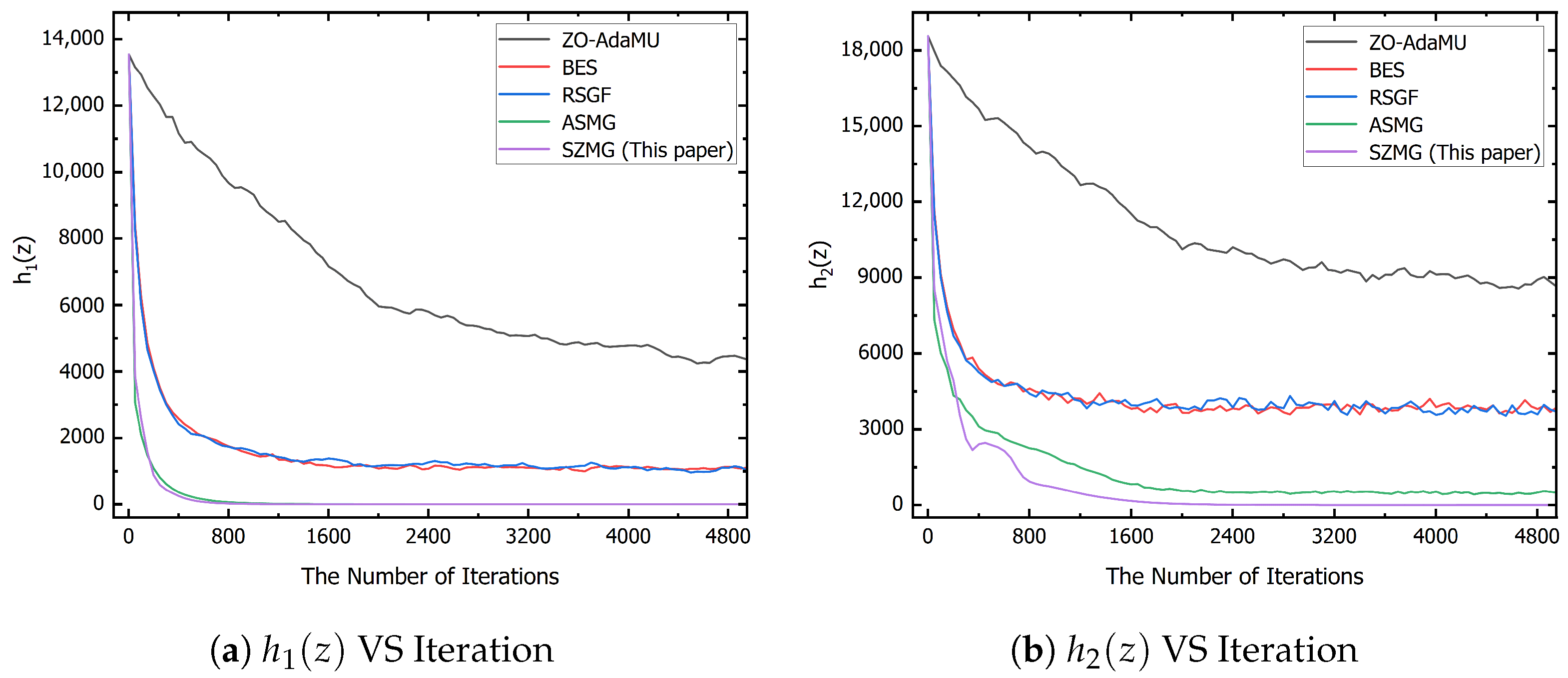
• Numerical experiments demonstrate the effectiveness of the SZMG algorithm.

The notations used in this paper are summarized in

Table 2. Some important notations used in the paper.

Notation	Introduction
z	Decision variable
w	Data random variable independence of z
u	A random vector following the Gaussian distribution
$\nu$	Smoothness parameter
d	The dimension of parameter z
M	Total number of functions
$h_i\left(z\right)$	The i-th objective function
$h_i^{\nu }\left(z\right)$	The smoothed version of function $h_i\left(z\right)$
$\nabla h_i\left(z\right)$	Gradient of the i-th objective function
$\nabla h_i^{\nu }\left(z\right)$	Gradient of the function $h_i^{\nu }\left(z\right)$
$s_i(z,u,w)$	Stochastic gradient of the function $h_i^{\nu }\left(z\right)$
$\nabla H\left(z\right)$	A matrix containing $\nabla h_1\left(z\right),\dots ,\nabla h_M\left(z\right)$ as columns
$\nabla H_{\nu }\left(z\right)$	A matrix containing $\nabla h_1^{\nu }\left(z\right),\dots ,\nabla h_M^{\nu }\left(z\right)$ as columns
$S_{\nu }(z,u,w)$	A matrix containing $s_1(z,u,w),\dots ,s_M(z,u,w)$ as columns
${\lambda }_t^{*}$	${\lambda }_t^{*}=arg{min}_{\lambda }{∥\nabla H\left(z_t\right)\lambda ∥}^2$
${\lambda }_{t,\nu }^{*}$	${\lambda }_{t,\nu }^{*}=arg{min}_{\lambda }{∥\nabla H_{\nu }\left(z_t\right)\lambda ∥}^2$
${\lambda }_{t,k+1}$	${\lambda }_{t,k+1}={\prod }_{{▵}^M}\left({\lambda }_{t,k}-{\beta }_{t,k}{S}_{\nu }{\left(z_t,u_t^{\prime },w_t^{\prime }\right)}^{\top }{S}_{\nu }\left(z_t,u_t^{″},w_t^{″}\right){\lambda }_{t,k}\right)$
$\eta ,\beta$	Learning rates
$c,l,L$	A constant greater than 0

.

2. Related Work

In this section, the development of gradient-based MOO and gradient-free MOO methods are briefly reviewed.

2.1. Gradient-Based Deterministic MOO

Gradient-based MOO methods can be divided into two categories—one is the scalarization method, as seen in References [15,16,26], which converts MOO problems into SOO problems by pre-selecting weights. Indeed, pre-selecting weights is a challenging task and does not resolve the issue of conflicting gradients. Another category is the non-scalarization method, which extends the ideas of SOO methods by finding a direction to optimize all objective functions simultaneously. Examples include the steepest descent method [27], the proximal method [28], Newton’s method [29], the trust-region method [30], and the conjugate gradient method [31]. Reference [18] proposes a dynamic weighting method called MGDA, which determines a descent direction in each iteration by solving a quadratic subproblem. After that, various MGDA variants have been studied, such as methods for obtaining Pareto distributions [19,20] and minimizing average loss [32]. However, the above studies focus on determination cases. In practical applications, stochastic and gradient-free cases remain challenges.

2.2. Gradient-Based Stochastic MOO

In recent years, the stochastic versions of MGDA have been studied. Reference [21] proposed SMGDA, but the paper did not identify an important property of SMGDA—that the stochastic multi-gradient direction is biased. This property was found in Reference [22], which provides a convergence analysis under strongly convex and convex settings by adopting a linearly increasing batch size. However, using a linearly increasing batch size is impractical. To tackle this challenge, various methods have been proposed to reduce stochastic multi-gradient bias, such as adopting momentum mechanisms [23,33], SGD-type methods [24], and double sampling [34,35]. However, these works all focus on situations where gradients are available. When encountering situations where the gradients of the function are not obtainable, these methods become ineffective.

2.3. Gradient-Free MOO

Many algorithms study black-box MOO problems, such as Bayesian optimization algorithms, as seen in [36,37]. These methods are better suited for handling low-dimensional expensive MOO problems. Another category is heuristic algorithms, such as [6,7,38]. These methods generally explore the entire Pareto solutions, which are computationally expensive and typically lack convergence guarantees. Recently, Reference [25] proposed a Hessian-aware zeroth-order optimization method, but the paper mainly focused on convex settings. Reference [13] proposed a multi-objective evolutionary strategy algorithm by iteratively updating the Gaussian distribution to find a Pareto solution. However, the paper assumes that the covariance matrix of the Gaussian distribution is diagonal, which is more suitable for separable functions. Additionally, achieving theoretical convergence guarantees requires that all function values be bounded, which is uncommon in standard SOO and MOO theoretical analysis. In this paper, we propose a zeroth-order multi-objective optimization algorithm (SZMG), which adopts a milder assumption. Additionally, the theoretical analysis of the SZMG algorithm is established under non-convex settings and milder assumptions. In the numerical experiments, the SZNG algorithm has demonstrated effectiveness in optimizing both separable and non-separable functions.

3. Preliminaries

In this section, the basic concept of MOO problems, the MGDA algorithm, and the zeroth-order gradient estimation methods are introduced.

3.1. Problem Setup

This paper addresses the following stochastic MOO problem:

$$\begin{array}{cc}\hfill \underset{z}{min}H\left(z\right)& =\left({\mathbb{E}}_w\left[h_1(z,w)\right],\dots ,{\mathbb{E}}_w\left[h_M(z,w)\right]\right),\hfill \end{array}$$

(1)

where $h_i:{\mathbb{R}}^d\to \mathbb{R}$ is the i-th continuously differentiable non-convex function with $h_m\left(z\right)={\mathbb{E}}_w\left[h_m(z,w)\right]$, z is a d-dimensional decision variable, w is a random variable, and M is the number of objective functions. In this setting, it is assumed that the gradients of the functions are not available, and only function values can be queried. Generally, the goal of MOO is to seek Pareto optimality, which means no other solution dominates it.

Definition 1 

(Pareto optimality). (a) For any two solutions, $z_1,z_2\in {\mathbb{R}}^d$, solution $z_1$ is said to dominate solution $z_2$, if $\forall i\in \left\{1,2,\dots ,M\right\}$, $h_i\left(z_1\right)\le h_i\left(z_2\right)$ and $H\left(z_1\right)\ne H\left(z_2\right)$. (b) A solution $z^{*}$ is called Pareto-optimal if no other solution dominates it.

For multi-objective non-convex functions, the goal is generally to find a Pareto stationary point, which is a necessary condition for the Pareto optimal point [23,24,33,39].

Definition 2 

(Pareto stationary point). If point z is a Pareto stationary point, then

$$range\left(\nabla H\left(z\right)\right)\cap \left(-{\mathbb{R}}_{++}^M\right)=\varnothing ,$$

where $\nabla H\left(z\right):=\left(\nabla h_1\left(z\right),\nabla h_2\left(z\right),\dots ,\nabla h_m\left(z\right)\right)$, and ${\mathbb{R}}_{++}^M$ is the positive orthant cone.

3.2. Multi-Gradient Descent Algorithm

The multi-gradient descent algorithm is a first-order gradient algorithm that aims to avoid conflicting gradients between functions. In each iteration, the algorithm first computes the gradients of the function, then obtains the descent direction $\nabla H\left(z\right){\lambda }^{*}\left(z\right)$, where weights ${\lambda }^{*}\left(z\right)={\left({\lambda }_1^{*}\left(z\right),\dots ,{\lambda }_M^{*}\left(z\right)\right)}^{\top }$ are acquired by solving the following sub-problem:

$$\begin{array}{cc}\hfill & {\lambda }^{*}\left(z\right)\in arg\underset{\lambda }{min}{∥\nabla H\left(z\right)\lambda ∥}^2\hfill \\ \hfill & s.t.\lambda \in {▵}^m:=\left\{\lambda \in {\mathbb{R}}^m|{\mathbf{1}}^{\top }\lambda =1,\lambda \ge 0\right\}.\hfill \end{array}$$

(2)

Then the parameter z is updated by the following equation:

$$\begin{array}{c}\hfill z_{t+1}=z_t-{\eta }_{t}d\left(z_t\right),\end{array}$$

(3)

where $d\left(z_t\right)=\nabla H\left(z_t\right){\lambda }^{*}\left(z_t\right)$ is the t-th iteration descent direction and ${\eta }_t$ is t-th iteration learning rate.

The standard MGDA is given in Algorithm 1, as follows:

Algorithm 1 Multi-gradient descent algorithm (MGDA)

1: Input: initial model parameter $z_0$, learning rate $\eta$. 2: for  $t=0,1,\dots ,T-1$  do 3:     for objective function $i=1,2,\dots ,M$ do 4:         Calculate gradients $\nabla h_i\left(z_t\right)$. 5:      end for 6:      Compute weights ${\lambda }^{*}\left(z_t\right)$ following (2). 7:      Update model parameters $z_{t+1}$ following (3). 8: end for

3.3. Zeroth-Order Optimization

ZOO is a method for approximating the gradient of a function by querying function values. Its fundamental idea is to use finite difference approximations of the directional derivatives of functions $h\left(z\right)$ along certain directions. In this paper, the Gaussian gradient estimator is utilized to approximate the gradients. For any function, $h_i\left(z\right)$, the Gaussian smoothed function of $h_i\left(z\right)$ is as follows:

$$h_i^{\nu }\left(z\right)={\mathbb{E}}_u\left[h_i(z+\nu u)\right],$$

(4)

where u follows the standard Gaussian distribution, $\nu$ is a smoothness parameter. The gradient of $h_i^{\nu }\left(z\right)$ can be expressed as follows:

$$\begin{array}{cc}\hfill \nabla h_i^{\nu }\left(z\right)& ={\mathbb{E}}_u\left[{\displaystyle \frac{h_i(z+\nu u)}{\nu }}u\right]\hfill \end{array}$$

(5)

$$\begin{array}{cc}\hfill & ={\mathbb{E}}_u\left[{\displaystyle \frac{h_i(z+\nu u)-h_i\left(z\right)}{\nu }}u\right],\hfill \end{array}$$

(6)

where Equation (5) is the single-point estimation and Equation (6) is the two-point estimation. In general, Equation (5) has a greater gradient variance than Equation (6) [40,41]. In this paper, two-point estimation is adopted to approximate the gradient.

4. Stochastic Zeroth-Order Multi-Gradient Algorithm

To address the challenge of unavailable gradients, this paper applies the ZOO technique to MOO problems. The multi-objective problem (1) is converted into a Gaussian smoothing multi-objective problem, as follows:

$$\begin{array}{c}\hfill \underset{z}{min}{H}_{\nu }\left(z\right)=\left(h_1^{\nu }\left(z\right),\dots ,h_M^{\nu }\left(z\right)\right),\end{array}$$

(7)

where $h_i^{\nu }\left(z\right)=\mathbb{E}\left[h_i(z+\nu u,w)\right]$. Following Equation (6), the stochastic gradient of the function $h_i^{\nu }\left(z\right)$ is defined as follows:

$$s_i(z,u,w)={\displaystyle \frac{1}{q_1{q}_2}}\sum _{m=1}^{q_1}\sum _{n=1}^{q_2}{\displaystyle \frac{h_i(z+\nu u_m,w_n)-h_i(z,w_n)}{\nu }}{u}_m.$$

(8)

In this paper, it is assumed that $\mathbb{E}\left[h_i\left(z,w\right)\right]=h_i\left(z\right)$, which indicates that the stochastic gradient $s_i(z,u,w)$ is an unbiased gradient estimation of $\nabla h_i^{\nu }\left(z\right)$ due to the following:

$$\begin{array}{cc}\hfill \mathbb{E}\left[s_i(z,u,w)\right]& ={\displaystyle \frac{1}{q_1{q}_2}}{\mathbb{E}}_u\left[{\mathbb{E}}_w\left[\sum _{m=1}^{q_1}\sum _{n=1}^{q_2}{\displaystyle \frac{h_i(z+\nu u_m,w_n)-h_i(z,w_n)}{\nu }}{u}_m|u\right]\right]\hfill \\ \hfill & ={\displaystyle \frac{1}{q_1{q}_2}}{\mathbb{E}}_u\left[\sum _{m=1}^{q_1}\sum _{n=1}^{q_2}{\displaystyle \frac{h_i(z+\nu u_m)-h_i\left(z\right)}{\nu }}{u}_m\right]\hfill \\ \hfill & =\nabla h_i^{\nu }\left(z\right).\hfill \end{array}$$

(9)

According to Equation (9), an unbiased stochastic gradient of function $h_i^{\nu }\left(z\right)$ can be obtained by querying the function values. To avoid potential conflicts in gradient direction, such as $〈s_i(z,u,w),s_j(z,u,w)〉<0$, the MGDA-type method is adopted to determine the weight values by solving the following problem:

$$\begin{array}{cc}\hfill & \underset{\lambda }{min}{∥\nabla H_{\nu }\left(z\right)\lambda ∥}^2\hfill \\ \hfill & s.t.\lambda \in {▵}^M:=\left\{\lambda \in {\mathbb{R}}^m|{\mathbf{1}}^{\top }\lambda =1,\lambda \ge 0\right\},\hfill \end{array}$$

(10)

where $\nabla H_{\nu }\left(z\right):=(\nabla h_1^{\nu }\left(z\right),\dots ,h_M^{\nu }\left(z\right))$.

According to References [22,33], replacing deterministic gradients $\nabla H_{\nu }\left(z\right)$ with stochastic gradients $S_{\nu }\left(z_{,}u,w\right)$ in Equation (10) and directly obtaining the weight values will introduce a bias $\mathbb{E}\left[S_{\nu }(z,u,w){\lambda }_{\nu }^{*}(z,u,w)\right]\ne \nabla H_{\nu }\left(z\right){\lambda }_{\nu }^{*}\left(z\right)$. To reduce this bias, an SGD-type method from [24] is adopted to obtain the optimal weight value ${\lambda }_{\nu }^{*}$.

The method for updating the weight ${\lambda }_t$ is as follows:

$$\begin{array}{c}\hfill {\lambda }_{t,k+1}={\prod }_{{▵}^M}\left({\lambda }_{t,k}-{\beta }_{t,k}{S}_{\nu }{\left(z_t,u_t^{\prime },w_t^{\prime }\right)}^{\top }{S}_{\nu }\left(z_t,u_t^{″},w_t^{″}\right){\lambda }_{t,k}\right),\end{array}$$

(11)

where $u_t^{\prime }$, $w_t^{\prime }$, $u_t^{″}$, $w_t^{″}$ are independent samples, ${\beta }_{t,k}$ is the learning rate for the weight ${\lambda }_t$ at the k-th iteration, and ${\prod }_{{▵}^M}$ represents a projection onto ${▵}^M$. The gradient $S_{\nu }{\left(z_t,u_t^{\prime },w_t^{\prime }\right)}^{\top }{S}_{\nu }\left(z_t,u_t^{″},w_t^{″}\right){\lambda }_{t,k}$ is unbiased for ${∥\nabla H_{\nu }\left(z\right)\lambda ∥}^2$ because

$$\begin{array}{c}\hfill \mathbb{E}\left[S_{\nu }{\left(z_t,u_t^{\prime },w_t^{\prime }\right)}^{\top }{S}_{\nu }\left(z_t,u_t^{″},w_t^{″}\right){\lambda }_{t,k}\right]=\nabla H_{\nu }{\left(z_t\right)}^{\top }\nabla H_{\nu }\left(z_t\right){\lambda }_{t,k}.\end{array}$$

(12)

After obtaining the weights, the decision variable $z_t$ will be updated by the following equation:

$$z_{t+1}=z_t-{\eta }_t{S}_{\nu }(z_t,u_t,w_t){\lambda }_{t,K},$$

(13)

where ${\eta }_t$ is the learning rate and K is the total number of iterations for the weight.

The proposed SZMG algorithm is given in Algorithm 2.

Algorithm 2 Stochastic zeroth-order multi-gradient algorithm (SZMG)

1: Input: initial model parameter $z_0$, weights ${\lambda }_0$, learning rates ${\left\{{\eta }_t\right\}}_{t=0}^T$, ${\left\{{\beta }_t\right\}}_{t=0}^T$. 2: for  $t=0,1,\dots ,T-1$  do 3:     Set weights ${\lambda }_{t,0}={\lambda }_{t-1,K}$. 4:     for $k=0,1,\dots ,K-1$ do 5:         Calculate zeroth-order gradient $S_{\nu }\left(z_t,u_t^{\prime },w_t^{\prime }\right)$, $S_{\nu }\left(z_t,u_t^{″},w_t^{″}\right)$. 6:         Update weights ${\lambda }_{t,k+1}$ following (11). 7:     end for 8:     Calculate zeroth-order gradient $S_{\nu }(z_t,u_t,w_t)$. 9:     Update model parameters $z_{t+1}$ following (13). 10: end for

5. Convergence Analysis

In this section, some standard assumptions are introduced first. Then, the error bound between gradient $S_{\nu }(z_t,u_t,w_t){\lambda }_{t,K}$ and gradient $\nabla H\left(z_t\right){\lambda }^{*}\left(z_t\right)$ is analyzed. Finally, the convergence rate of the SZMG algorithm is established. All the proofs are put in Appendix B.

Assumption 1. 

For any $z\in {\mathbb{R}}^d$, the estimation of $h_i\left(z\right)$ is unbiased such that ${\mathbb{E}}_w\left[h_i(z,w)\right]=h_i\left(z\right)$.

This assumption ensures that Equation (9) holds, making $s_i(z,u,w)$ an unbiased estimate of the gradients $\nabla h_i^{\nu }\left(z\right)$. This is also a standard assumption in stochastic zeroth-order optimization [12,40,42].

Assumption 2. 

All functions $h_1(z,w),\dots ,h_M(z,w)$ are l-Lipschitz continuous for any w and $h_1\left(z\right),\dots ,h_M\left(z\right)$ are L-smoothness, i.e.,

$$∥\nabla h_i(z_1,w)∥\le l,$$

$$h_i\left(z_1\right)\le h_i\left(z_2\right)+〈\nabla h_i\left(z_2\right),z_1-z_2〉+{\displaystyle \frac{L}{2}}{∥z_1-z_2∥}^2,$$

for any $z_1,z_2\in {\mathbb{R}}^d$.

Applying Jensen’s inequality, we have the following:

$${∥\nabla h_i\left(z\right)∥}^2\le \mathbb{E}\left[{∥\nabla h_i(z,w)∥}^2\right]\le l^2,$$

(14)

which implies that functions $h_1\left(z\right),\dots ,h_M\left(z\right)$ are l-Lipschitz continuous.

This is a standard assumption in MOO problems [23,24]. Here, the assumption that $h_i(z,w)$ is l-Lipschitz continuous is to ensure that gradient $s_i(z,u,w)$ is bounded for all $i\in \left\{1,\dots ,M\right\}$, which is necessary to control the drift of the optimal weight $\lambda$, thereby establishing convergence guarantees in the non-convex setting. This assumption is used for zeroth-order stochastic optimization problems in [12,43]. The L-smoothness property of the function is a standard assumption used to establish the convergence of non-convex functions [44].

Assumption 3. 

For some $\lambda \in {▵}^M$, there exists a constant $C_H$ such that $H_{\nu }\left(z_0\right)\lambda -{min}_z{H}_{\nu }\left(z\right)\lambda \le C_H$.

This assumption implies that there exists at least an objective function that is bounded at the initial point, such as $h_i^{\nu }\left(z_0\right)-{min}_z{h}_i^{\nu }\left(z\right)\le C_H$, which implies that the distance between the initial point and the Pareto optimal solution is finite. From this, it can be inferred that the algorithm can converge to the Pareto solution within a reasonable amount of time. Compared to [13], which requires the function values bounded for all objective functions at any point z, this is a milder assumption.

These assumptions are typically reasonable in the context of black-box adversarial attacks on an image classification neural network model. For example, in [45], the sparse adversarial attack is transformed into a multi-objective black-box optimization problem. In this context, the aforementioned assumptions hold.

The error upper bound between $S_{\nu }(z_t,u_t,w_t){\lambda }_{t,K}$ and $\nabla H\left(z_t\right){\lambda }^{*}\left(z_t\right)$ is established as follows:

Proposition 1. 

Suppose Assumptions 1 and 2 are satisfied. If we set $\nu =\Theta ({\displaystyle \frac{1}{\sqrt{T}d}})$, $K=T^2$, $\sqrt{d}\le q_1{q}_2<d$, and ${\beta }_{t,k}={\displaystyle \frac{c}{\sqrt{k}}}$, where $c>0$ is a constant, we have the following:

$$\begin{array}{cc}\hfill & \mathbb{E}\left[{∥\mathbb{E}\left[S_{\nu }\left(z_t,u_t,w_t\right){\lambda }_{t,K}\right]-\nabla H\left(z_t\right){\lambda }_t^{*}∥}^2|z_t\right]\hfill \\ \hfill \le & {\displaystyle \frac{c(log(K)+2)}{\sqrt{K}}}{\left({\displaystyle \frac{M{\nu }^2}{2q_1{q}_2}}{L}^2{(d+6)}^3+{\displaystyle \frac{2d+9+q_1{q}_2}{q_1{q}_2}}M{l}^2\right)}^2\hfill \\ \hfill & +\left(log\left(K\right)+2\right)\left({\displaystyle \frac{1}{c\sqrt{K}}}+\sqrt{2}\nu MLl{(d+3)}^{3/2}\right)+{\displaystyle \frac{M{\nu }^2}{4}}{L}^2{(d+3)}^3\hfill \\ \hfill =& \mathcal{O}\left({\displaystyle \frac{log\left(K\right)\sqrt{d}}{K^{1/4}}}\right).\hfill \end{array}$$

(15)

Proposition 1 shows that the error bound will converge to 0 as $K\to \infty$. The following theorem shows the SZMG can converge to a Pareto stationary point under a non-convex setting and mild assumptions:

Theorem 1. 

Suppose Assumptions 1, 2, and 3 are satisfied. If we set $\eta =\Theta (T^{-{\displaystyle \frac{1}{2}}})$, $\nu =\Theta ({\displaystyle \frac{1}{\sqrt{T}d}})$$K=\Theta (T^2)$, $\sqrt{d}\le q_1{q}_2<d$, and ${\beta }_{t,k}={\displaystyle \frac{c}{\sqrt{k}}}$, where $c>0$ is a constant, we have the following:

$$\begin{array}{cc}\hfill & {\displaystyle \frac{1}{T}}\sum _{t=0}^{T-1}\mathbb{E}\left[{∥\nabla H\left(z_t\right){\lambda }_t^{*}∥}^2\right]\hfill \\ \hfill \le & {\displaystyle \frac{2C_H}{T\eta }}+4l\sqrt{{\displaystyle \frac{1+log\left(T\right)}{cT}}}+{\displaystyle \frac{M{\nu }^2}{2}}{L}^2{(d+3)}^3\hfill \\ \hfill & +{\displaystyle \frac{M{\nu }^2}{2q_1{q}_2}}{L}^2{(d+6)}^3\left(2l\sqrt{{\displaystyle \frac{2c+2clog\left(T\right)}{T}}}+L\eta \right)\hfill \\ \hfill & +{\displaystyle \frac{2d+9+q_1{q}_2}{q_1{q}_2}}M{l}^2\left(2l\sqrt{{\displaystyle \frac{2c+2clog\left(T\right)}{T}}}+L\eta \right)\hfill \\ \hfill =& \mathcal{O}\left({\displaystyle \frac{d\sqrt{log\left(T\right)}}{q_1{q}_2\sqrt{T}}}\right).\hfill \end{array}$$

(16)

Theorem 1 shows that the proposed SZMG algorithm converges to a Pareto stationary point with a convergence rate of $\mathcal{O}({\displaystyle \frac{d\sqrt{log(T)}}{q_1{q}_2\sqrt{T}}})$. By choosing the parameter $q_1{q}_2=\sqrt{d}$ and ignoring the term $\sqrt{log\left(T\right)}$, which grows very slowly, the convergence rate of the SZMG algorithm reaches $\mathcal{O}(\sqrt{d}/\sqrt{T})$, which indicates that the SZMG algorithm has a convergence rate that matches the one in the zeroth-order stochastic single-objective non-convex setting [12]. To achieve an $ϵ$-optimal solution, the query complexity for each objective function is bounded by $\mathcal{O}\left(d^{9/2}/{ϵ}^6\right)$.

To reduce function query complexity, the error between $S_{\nu }(z_t,u_t,w_t){\lambda }_{t,K}$ and $\nabla H\left(z_t\right){\lambda }^{*}\left(z_t\right)$ is not considered. The following theorem shows that the query complexity for converging to an $ϵ$-optimal solution is bounded by $\mathcal{O}\left(d^{{\displaystyle \frac{3}{2}}}/{ϵ}^2\right)$.

Theorem 2. 

Suppose Assumptions 1–3 are satisfied. If we set $\eta =\Theta (T^{-{\displaystyle \frac{1}{2}}})$, $\beta =\Theta (T^{-{\displaystyle \frac{1}{2}}}{d}^{-{\displaystyle \frac{1}{2}}})$, $\nu =\Theta (T^{-{\displaystyle \frac{1}{2}}}{d}^{-1})$, $\sqrt{d}\le q_1{q}_2<d$, and $K=1$, we have the following:

$$\begin{array}{cc}\hfill & {\displaystyle \frac{1}{T}}\sum _{t=0}^{T-1}\mathbb{E}\left[{∥\nabla H\left(z_t\right){\lambda }_t^{*}∥}^2\right]\hfill \\ \hfill \le & {\displaystyle \frac{2C_H}{T\eta }}+\beta {\left({\displaystyle \frac{M{\nu }^2}{2q_1{q}_2}}{L}^2{(d+6)}^3+{\displaystyle \frac{2d+9+q_1{q}_2}{q_1{q}_2}}M{l}^2\right)}^2+{\displaystyle \frac{2}{T\beta }}\hfill \\ \hfill & +\eta L\left({\displaystyle \frac{M{\nu }^2}{2q_1{q}_2}}{L}^2{(d+6)}^3+{\displaystyle \frac{2d+9+q_1{q}_2}{q_1{q}_2}}M{l}^2\right)+{\displaystyle \frac{M{\nu }^2}{2}}{L}^2{(d+3)}^3\hfill \\ \hfill =& \mathcal{O}\left({\displaystyle \frac{d^{\frac{3}{2}}}{T^{\frac{1}{2}}{\left(q_1{q}_2\right)}^2}}\right).\hfill \end{array}$$

(17)

If we set the parameter $q_1{q}_2=\sqrt{d}$, Theorem 2 shows that the SZMG algorithm converges to a Pareto stationary point with a convergence rate of $\mathcal{O}(\sqrt{d}/\sqrt{T})$. To achieve an $ϵ$-optimal solution, the query complexity for each function is bounded by $\mathcal{O}(d^{{\displaystyle \frac{3}{2}}}/{ϵ}^2)$.

6. Experiments

In this section, several synthesis experiments are organized to verify the performance of the proposed SZMG algorithm.

6.1. Toy Example

To demonstrate that the proposed SZMG algorithm achieves better performance in stochastic multi-objective black-box settings, the first synthesis experiment is a two-dimensional problem, which is used in [34]. The objective functions are defined as follows:

$$\begin{array}{cc}\hfill & h_1\left(z\right)=f_1\left(z\right)g_1\left(z\right)+f_2\left(z\right)c_1\left(z\right)\hfill \end{array}$$

(18)

$$\begin{array}{cc}\hfill & h_2\left(z\right)=f_1\left(z\right)g_2\left(z\right)+f_2\left(z\right)c_2\left(z\right),\hfill \end{array}$$

(19)

where the functions $f_1\left(z\right)$, $f_2\left(z\right)$, $g_1\left(z\right)$, $g_2\left(z\right)$, $c_1\left(z\right)$, and $c_2\left(z\right)$ are defined by the following equations:

$$\begin{array}{cc}\hfill f_1\left(z\right)=& max\left(tanh\left(0.5z_2\right),0\right)\hfill \\ \hfill f_2\left(z\right)=& max\left(tanh(-0.5z_2),0\right)\hfill \\ \hfill c_1\left(z\right)=& \left({(-z_1+3.5)}^2+0.1{(-z_2-1)}^2\right)/10-20\hfill \\ \hfill & -2z_1{w}_1-5.5z_2{w}_2\hfill \\ \hfill c_2\left(z\right)=& \left({(-z_1-3.5)}^2+0.1{(-z_2-1)}^2\right)/10-20\hfill \\ \hfill & +2z_1{w}_1-5.5z_2{w}_2\hfill \\ \hfill g_1\left(z\right)=& log\left(max\left(|0.5(-z_1-7)-tanh(-z_2)|,\right.\right.\hfill \\ & \left.\left.0.000005\right)\right)+6\hfill \\ \hfill g_2\left(z\right)=& log\left(max\left(|0.5(-z_1+3)-tanh(-z_2)+2|,\right.\right.\hfill \\ \hfill & \left.\left.0.000005\right)\right)+6,\hfill \end{array}$$

where $z={[z_1,z_2]}^{\top }\in {\mathbb{R}}^2$ is the model parameter, and $w={[w_1,w_2]}^{\top }\in {\mathbb{R}}^2$ represents stochastic data, which follow the standard Gaussian distribution, as follows:

The following three initial points are selected:

$$z_0\in \{(-8.5,7.5),(-10,-3),(9,9)\}$$

The optimization trajectories of ZO-AdaMU (zeroth-order adapt momentum and uncertainty) [10], BES (Bernoulli smoothing) [11], RSGF (randomized stochastic gradient-free) [12], ASMG (adaptive stochastic multi-objective gradient) [13], MGDA [18], and SZMG are plotted in Figure 1. RSGF uses the Gaussian gradient estimator and BES adopts the variant of the Bernoulli distribution to estimate the gradient. ZO-AdaMU adopts the Gaussian gradient estimator by adapting perturbation with momentum and uncertainty. These three algorithms primarily focus on single-objective problems. In multi-objective scenarios, multiple objectives are aggregated into a single objective by applying equal weights to each individual objective. ASMG is an adaptive multi-objective gradient algorithm based on evolutionary strategies. MGDA is a first-order gradient algorithm. All algorithms adopt the Adam optimizer and the number of iterations is $T=70,000$. Other hyperparameters are summarized in

Table 3. Summary of hyperparameters.

	$\mathit{\nu }$	${\mathit{q}}_1$	${\mathit{q}}_2$	$\mathit{\eta }$	K	$\mathit{\gamma }$	$\mathit{\beta }$
ZO-AdaMU	0.00001	8	8	0.002	-	-	-
BES	0.00001	8	8	0.002	-	-	-
RSGF	0.00001	8	8	0.002	-	-	-
ASMG	-	8	8	0.01	-	${\displaystyle \frac{1}{t+1}}$	-
MGDA	-	-	full	0.002	-	-	-
SZMG	0.00001	8	8	0.002	1	-	${\displaystyle \frac{0.01}{\sqrt{k}}}$

.

In Figure 1, the results show that algorithms SZMG and ASMG can effectively optimize stochastic multi-objective black-box functions while addressing the conflicting gradient problem. The three initial points have all converged to the Pareto front. In contrast, the ZO-AdaMU, BES, and RSGF methods all become trapped in a valley at initial points $(-8,5,7.5),(9,9)$, and fail to reach the Pareto front due to the dominant gradient of a specific objective.

Figure 2 examines the impact of different numbers of inner iterations K on the error between gradients $S_{\nu }(z_t,u_t,w_t){\lambda }_{t,K}$, and $\nabla H\left(z_t\right){\lambda }^{*}\left(z_t\right)$. The gradient deviation for each trajectory is measured using the average norm ${\displaystyle \frac{1}{T}}{\sum }_{t=1}^T∥S_{\nu }(z_t,u_t,w_t){\lambda }_{t,K}-\nabla H\left(z_t\right){\lambda }^{*}\left(z_t\right)∥$. From the results, it can be seen that as K increases, the gradient deviation becomes smaller. This result validates Proposition 1. In Figure 1, the optimization trajectories of the SZMG algorithm are presented for different numbers of inner iterations K.

6.2. Separable and Non-Separable Functions

To validate the performance of the proposed SZMG algorithm under separable and non-separable functions, SZMG is compared to other algorithms using synthetic functions in 500 and 1000 dimensions.

For separable functions, we have the following:

$$\begin{array}{cc}\hfill H\left(z\right)& =(h_1\left(z\right),h_2\left(z\right))\hfill \\ \hfill & =\left(\sum _{i=1}^d{10}^{{\displaystyle \frac{2(i-1)}{d-1}}}{z}_i^2,10d-\sum _{i=1}^{d}10cos(2\pi {10}^{{\displaystyle \frac{(i-1)}{d-1}}}{z}_i)+\sum _{i=1}^d{({10}^{{\displaystyle \frac{(i-1)}{d-1}}}{z}_i)}^2\right).\hfill \end{array}$$

(20)

For non-separable functions, we have the following:

$$\begin{array}{c}\hfill H\left(x\right)=H\left(Rz\right)=\left(h_1\left(x\right),h_2\left(x\right)\right),\end{array}$$

(21)

where $h_1\left(x\right)={\sum }_{i=1}^d{x}_i^2-10cos\left(2\pi x_i\right)+10$, $h_2\left(x\right)={\displaystyle \frac{1}{d}}{\sum }_{i=1}^{d-1}100{\left(x_i^2-x_{i+1}\right)}^2+{\left(x_i-4\right)}^2$, and R is an orthogonal matrix generated by applying the Gram–Schmidt procedure to a random matrix with a standard normal distribution.

The SZMG algorithm will be compared with ZO-AdaMU [10], BES [11], RSGF [12], and ASMG [13]. For ZO-AdaMU, BES, RSGF, and SZMG methods, the learning rate is selected from $\{0.01,0.005,0.001,0.0005,0.0001,0.00005,0.00001\}$, and the smoothing parameters $\nu$ is set to $0.00001$. In the SZMG algorithm, the weight learning rate $\beta$ is set to $0.005$, and the number of inner iterations K is set to 1. The ASMG algorithm selects the learning rate from $\{5,1,0.5,0.1,0.05\}$. The total number of iterations T and the sample batch size $q_1$ are set to 5000 and 50, respectively, for all algorithms.

In Figure 3 and Figure 4, the convergence results of five algorithms on the separable function under different dimensions are presented. Specifically, the function value with respect to the number of iterations is presented. The results demonstrate that the proposed SZMG algorithm achieves better performance. The ASMG algorithm exhibits faster convergence on the separable function. ZO-AdaMU, BES, and RSGF methods converge to a suboptimal Pareto solution due to conflicting gradients. In Figure 5 and Figure 6, the convergence results of five algorithms on the non-separable functions under different dimensions are presented. The results can intuitively show that the SZMG algorithm outperforms ASMG in terms of convergence performance and results. These results show that the SZMG algorithm performs well on both separable and non-separable functions, demonstrating the effectiveness of the SZMG algorithm.

6.2.1. Runtime

In this subsection, the runtimes of different algorithms on separable functions are compared to evaluate their computational complexity. The runtime of an algorithm is the average time per iteration over 5000 iterations. The experimental results were obtained using a PC equipped with a 3.60-GHz Intel Core i7-7700 CPU (Acer, Luoyang, China).

Figure 7 shows the average time per iteration for the methods ZO-AdaMU, BES, RSGF, ASMG, and SZMG across different dimensions of separable functions. From the results, the BES and RSGF methods have the shortest runtime per iteration because they do not need to compute weights. ZO-AdaMU takes the longest time due to requiring multiple uncertain perturbations internally. SZMG requires an additional gradient estimation and matrix operation to obtain the weights, making its runtime longer than RSGF. Compared to ASMG, SZMG has a shorter runtime, which indicates that the SZMG has better efficiency.

6.2.2. Scalability

In this subsection, the scalability of SZMG is studied on separable and non-separable functions at 1500 and 3000 dimensions.

Figure 8 and Figure 9 show the convergence results of algorithms ZO-AdaMU, BES, RSGF, ASMG, and SZMG on separable functions at 1500 and 3000 dimensions. These results indicate that the SZMG algorithm has better performance and can converge to the Pareto solutions. Figure 10 and Figure 11 present the convergence results on non-separable functions at 1500 and 3000 dimensions. These results show that SZMG delivers better performance, which implies that gradient-based optimization methods are better suited for handling high-dimensional problems; moreover, using dynamic weights based on SGD effectively addresses conflicting gradients. These results demonstrate the SZMG algorithm’s effectiveness.

6.2.3. Sensitiveness to Batch Size

The sample batch size is a key parameter in the proposed SZMG algorithm. A larger batch size can reduce the variance of zeroth-order gradients, leading to a more accurate gradient direction, but it also results in higher time and function query overheads. In this subsection, we study the impact of different batch sizes on the convergence of the SZMG algorithm for non-separable functions.

Figure 12 shows the impact of batch sizes 10, 30, 50, and 70 on the SAMG algorithm for the 1000-dimensional non-separable function. From the results, it can be observed that as the batch size increases, the convergence trajectory of the SZMG algorithm becomes more stable and the convergence improves. Figure 13 shows the average runtime per iteration for different batch sizes. The runtime increases linearly with the batch size. Therefore, careful selection of an appropriate batch size is critical for balancing time consumption and stability for the SZMG algorithm.

7. Discussion

In the experiments section, several numerical experiments were conducted to validate the practical performance of the proposed SZMG algorithm. The results show that SZMG demonstrates promising performance on smooth black-box functions. As a zeroth-order variant of first-order multi-objective optimization algorithms, SZMG exhibits a convergence rate comparable to first-order methods and can serve as a substitute for these algorithms in handling black-box multi-objective optimization problems or scenarios with expensive gradients. Theoretically, we have demonstrated that the convergence rate of SZMG is $\mathcal{O}\left(d\right)$ worse than the first-order multi-objective optimization methods.

Despite its advantages, SZMG has potential limitations such as the curse of dimensionality. As the dimensionality of the problem increases, the number of required function evaluations also rises significantly, leading to a sharp increase in computational costs. Additionally, the theoretical convergence guarantees of SZMG are based on smooth functions, and its performance may degrade when applied to non-smooth functions. These limitations are also important research directions for zeroth-order multi-objective optimization algorithms.

In real-world applications, the SZMG algorithm has a wide range of application scenarios, such as black-box adversarial attacks. In single-objective optimization, zeroth-order algorithms are widely used in black-box attacks and have achieved excellent results [46]. Recently, Reference [45] explored sparse adversarial attacks as multi-objective problems, employing heuristic algorithms to generate adversarial examples. There is significant potential for applying the SZMG algorithm in this field.

8. Conclusions

In this paper, a gradient-free stochastic multi-objective optimization algorithm is proposed for addressing black-box multi-objective optimization problems. The algorithm applies zeroth-order optimization techniques to multi-objective optimization and adopts a dynamic weighting method to avoid conflicting gradients. Theoretically, this paper provides a convergence guarantee for the proposed algorithm under non-convex settings and mild assumptions. Moreover, synthetic experiments demonstrate the effectiveness of the proposed algorithm. In the future, it will be valuable to explore methods for zeroth-order algorithms to handle high-dimensional problems and introduce variance reduction techniques into zeroth-order optimization to reduce gradient variance and achieve better convergence performance.

References

1. Lu, W.; Zhou, Y.; Wan, G.; Hou, S.; Song, S. L3-Net: Towards Learning Based LiDAR Localization for Autonomous Driving. In Proceedings of the 31th IEEE Conference on Computer Vision and Pattern Recognition, CVPR, Long Beach, CA, USA, 16–20 June 2019. [Google Scholar]
2. Fernandes, P.; Ghorbani, B.; Garcia, X.; Freitag, M.; Firat, O. Scaling Laws for Multilingual Neural Machine Translation. In Proceedings of the 40th International Conference on Machine Learning, ICML, Honolulu, HI, USA, 23–29 July 2023. [Google Scholar]
3. Satija, H.; Thomas, P.S.; Pineau, J.; Laroche, R. Multi-Objective SPIBB: Seldonian Offline Policy Improvement with Safety Constraints in Finite MDPs. In Proceedings of the 35th Advances in Neural Information Processing Systems, NeurIPS, Virtual, 6–14 December 2021. [Google Scholar]
4. Zhang, L.; Liu, X.; Mahmood, K.; Ding, C.; Guan, H. Dynamic Gradient Balancing for Enhanced Adversarial Attacks on Multi-Task Models. CoRR 2023. [Google Scholar] [CrossRef]
5. Cui, Y.; Geng, Z.; Zhu, Q.; Han, Y. Review: Multi-objective optimization methods and application in energy saving. Energy 2017, 125, 681–704. [Google Scholar] [CrossRef]
6. Deb, K.; Agrawal, S.; Pratap, A.; Meyarivan, T. A fast and elitist multiobjective genetic algorithm: NSGA-II. IEEE Trans. Evol. Comput. 2002, 6, 182–197. [Google Scholar] [CrossRef]
7. Coello, C.A.C.; Pulido, G.T.; Lechuga, M.S. Handling Multiple Objectives With Particle Swarm Optimization. IEEE Trans. Evol. Comput. 2004, 8, 256–279. [Google Scholar] [CrossRef]
8. Mirjalili, S.; Saremi, S.; Mirjalili, S.M.; dos Santos Coelho, L. Multi-objective grey wolf optimizer: A novel algorithm for multi-criterion optimization. Expert Syst. Appl. 2016, 47, 106–119. [Google Scholar] [CrossRef]
9. Bandyopadhyay, S.; Saha, S.; Maulik, U.; Deb, K. A Simulated Annealing-Based Multiobjective Optimization Algorithm: AMOSA. IEEE Trans. Evol. Comput. 2008, 12, 269–283. [Google Scholar] [CrossRef]
10. Jiang, S.; Chen, Q.; Pan, Y.; Xiang, Y.; Lin, Y.; Wu, X.; Liu, C.; Song, X. ZO-AdaMU Optimizer: Adapting Perturbation by the Momentum and Uncertainty in Zeroth-Order Optimization. In Proceedings of the 38th AAAI Conference on Artificial Intelligence, AAAI, Vancouver, BC, Canada, 20–27 February 2024. [Google Scholar] [CrossRef]
11. Gao, K.; Sener, O. Generalizing Gaussian Smoothing for Random Search. In Proceedings of the 39th International Conference on Machine Learning, ICML, Baltimore, MD, USA, 17–23 July 2022. [Google Scholar]
12. Ghadimi, S.; Lan, G. Stochastic First- and Zeroth-Order Methods for Nonconvex Stochastic Programming. SIAM J. Optim. 2013, 23, 2341–2368. [Google Scholar] [CrossRef]
13. Ye, F.; Lyu, Y.; Wang, X.; Zhang, Y.; Tsang, I.W. Adaptive Stochastic Gradient Algorithm for Black-box Multi-Objective Learning. In Proceedings of the 12th International Conference on Learning Representations, ICLR, Vienna, Austria, 7–11 May 2024. [Google Scholar]
14. Zerbinati, A.; Desideri, J.A.; Duvigneau, R. Comparison Between MGDA and PAES for Multi-Objective Optimization; Research Report RR-7667; INRIA: Le Chesnay-Rocquencourt, France, 2011. [Google Scholar]
15. Gass, S.; Saaty, T. The computational algorithm for the parametric objective function. Nav. Res. Logist. 1955, 2, 39–45. [Google Scholar] [CrossRef]
16. Haimes, Y. On a bicriterion formulation of the problems of integrated system identification and system optimization. IEEE Trans. Syst. Man Cybern. Syst. 1971, SMC-1, 296–297. [Google Scholar] [CrossRef]
17. Chen, Z.; Ngiam, J.; Huang, Y.; Luong, T.; Kretzschmar, H.; Chai, Y.; Anguelov, D. Just Pick a Sign: Optimizing Deep Multitask Models with Gradient Sign Dropout. In Proceedings of the 34th Advances in Neural Information Processing Systems, NeurIPS, Virtual, 6–12 December 2020. [Google Scholar]
18. Désidéri, J.A. Multiple-gradient descent algorithm (MGDA) for multiobjective optimization. C. R. Math. 2012, 350, 313–318. [Google Scholar] [CrossRef]
19. Lin, X.; Zhen, H.; Li, Z.; Zhang, Q.; Kwong, S. Pareto Multi-Task Learning. In Proceedings of the 33th Advances in Neural Information Processing Systems, NeurIPS, Vancouver, BC, Canada, 8–14 December 2019. [Google Scholar]
20. Mahapatra, D.; Rajan, V. Multi-Task Learning with User Preferences: Gradient Descent with Controlled Ascent in Pareto Optimization. In Proceedings of the 37th International Conference on Machine Learning, ICML, Virtual Event, 13–18 July 2020. [Google Scholar]
21. Mercier, Q.; Poirion, F.; Désidéri, J. A stochastic multiple gradient descent algorithm. Eur. J. Oper. Res. 2018, 271, 808–817. [Google Scholar] [CrossRef]
22. Liu, S.; Vicente, L.N. The stochastic multi-gradient algorithm for multi-objective optimization and its application to supervised machine learning. Ann. Oper. Res. 2024, 339, 1119–1148. [Google Scholar] [CrossRef]
23. Zhou, S.; Zhang, W.; Jiang, J.; Zhong, W.; Gu, J.; Zhu, W. On the Convergence of Stochastic Multi-Objective Gradient Manipulation and Beyond. In Proceedings of the 36th Advances in Neural Information Processing Systems, NeurIPS, New Orleans, LA, USA, 28 November–9 December 2022. [Google Scholar]
24. Xiao, P.; Ban, H.; Ji, K. Direction-oriented Multi-objective Learning: Simple and Provable Stochastic Algorithms. In Proceedings of the 37the Advances in Neural Information Processing Systems, NeurIPS, New Orleans, LA, USA, 10–16 December 2023. [Google Scholar]
25. Chen, R.; Li, Y.; Chai, T. Multi-Objective Derivative-Free Optimization Based on Hessian-Aware Gaussian Smoothing Method. In Proceedings of the 18th IEEE International Conference on Control & Automation, ICCA, Reykjavík, Iceland, 18–21 June 2024. [Google Scholar] [CrossRef]
26. Tammer, C.; Winkler, K. A new scalarization approach and applications in multicriteria d.c. optimization. J. Nonlinear Convex Anal. 2003, 4, 365–380. [Google Scholar]
27. Fliege, J.; Svaiter, B.F. Steepest descent methods for multicriteria optimization. Math. Methods Oper. Res. 2000, 51, 479–494. [Google Scholar] [CrossRef]
28. Bonnel, H.; Iusem, A.N.; Svaiter, B.F. Proximal Methods in Vector Optimization. SIAM J. Optim. 2005, 15, 953–970. [Google Scholar] [CrossRef]
29. Fliege, J.; Drummond, L.M.G.; Svaiter, B.F. Newton’s Method for Multiobjective Optimization. SIAM J. Optim. 2009, 20, 602–626. [Google Scholar] [CrossRef]
30. Carrizo, G.A.; Lotito, P.A.; Maciel, M.C. Trust region globalization strategy for the nonconvex unconstrained multiobjective optimization problem. Math. Program. 2016, 159, 339–369. [Google Scholar] [CrossRef]
31. Pérez, L.R.L.; da Fonseca Prudente, L. Nonlinear Conjugate Gradient Methods for Vector Optimization. SIAM J. Optim. 2018, 28, 2690–2720. [Google Scholar] [CrossRef]
32. Liu, L.; Li, Y.; Kuang, Z.; Xue, J.; Chen, Y.; Yang, W.; Liao, Q.; Zhang, W. Towards Impartial Multi-task Learning. In Proceedings of the 9th International Conference on Learning Representations, ICLR, Virtual Event, 3–7 May 2021. [Google Scholar]
33. Fernando, H.D.; Shen, H.; Liu, M.; Chaudhury, S.; Murugesan, K.; Chen, T. Mitigating Gradient Bias in Multi-objective Learning: A Provably Convergent Approach. In Proceedings of the 11th International Conference on Learning Representations, ICLR, Kigali, Rwanda, 1–5 May 2023. [Google Scholar]
34. Chen, L.; Fernando, H.D.; Ying, Y.; Chen, T. Three-Way Trade-Off in Multi-Objective Learning: Optimization, Generalization and Conflict-Avoidance. J. Mach. Learn. Res. 2024, 25, 193:1–193:53. [Google Scholar]
35. Fernando, H.D.; Chen, L.; Lu, S.; Chen, P.; Liu, M.; Chaudhury, S.; Murugesan, K.; Liu, G.; Wang, M.; Chen, T. Variance Reduction Can Improve Trade-Off in Multi-Objective Learning. In Proceedings of the 49th IEEE International Conference on Acoustics, Speech and Signal Processing, ICASSP, Seoul, Republic of Korea, 14–19 April 2024. [Google Scholar] [CrossRef]
36. Laumanns, M.; Ocenasek, J. Bayesian Optimization Algorithms for Multi-objective Optimization. In Proceedings of the 7th Parallel Problem Solving from Nature, PPSN, Granada, Spain, 7–11 September 2002. [Google Scholar] [CrossRef]
37. Belakaria, S.; Deshwal, A.; Jayakodi, N.K.; Doppa, J.R. Uncertainty-Aware Search Framework for Multi-Objective Bayesian Optimization. In Proceedings of the 34th AAAI Conference on Artificial Intelligence, AAAI, New York, NY, USA, 7–12 February 2020. [Google Scholar] [CrossRef]
38. Zhang, Q.; Li, H. MOEA/D: A Multiobjective Evolutionary Algorithm Based on Decomposition. IEEE Trans. Evol. Comput. 2007, 11, 712–731. [Google Scholar] [CrossRef]
39. Fliege, J.; Vaz, A.I.F.; Vicente, L.N. Complexity of gradient descent for multiobjective optimization. Optim. Methods Softw. 2019, 34, 949–959. [Google Scholar] [CrossRef]
40. Liu, S.; Chen, P.; Kailkhura, B.; Zhang, G.; III, A.O.H.; Varshney, P.K. A Primer on Zeroth-Order Optimization in Signal Processing and Machine Learning: Principals, Recent Advances, and Applications. IEEE Signal Process. Mag. 2020, 37, 43–54. [Google Scholar] [CrossRef]
41. Berahas, A.S.; Cao, L.; Choromanski, K.; Scheinberg, K. A Theoretical and Empirical Comparison of Gradient Approximations in Derivative-Free Optimization. Found. Comput. Math. 2022, 22, 507–560. [Google Scholar] [CrossRef]
42. Balasubramanian, K.; Ghadimi, S. Zeroth-Order Nonconvex Stochastic Optimization: Handling Constraints, High Dimensionality, and Saddle Points. Found. Comput. Math. 2022, 22, 35–76. [Google Scholar] [CrossRef]
43. Chen, X.; Liu, S.; Xu, K.; Li, X.; Lin, X.; Hong, M.; Cox, D.D. ZO-AdaMM: Zeroth-Order Adaptive Momentum Method for Black-Box Optimization. In Proceedings of the 33th Advances in Neural Information Processing Systems, NeurIPS, Vancouver, BC, Canada, 8–14 December 2019. [Google Scholar]
44. Bottou, L.; Curtis, F.E.; Nocedal, J. Optimization Methods for Large-Scale Machine Learning. SIAM Rev. 2018, 60, 223–311. [Google Scholar] [CrossRef]
45. Williams, P.N.; Li, K. Black-Box Sparse Adversarial Attack via Multi-Objective Optimisation CVPR Proceedings. In Proceedings of the IEEE/CVF Conference on Computer Vision and Pattern Recognition, CVPR 2023, Vancouver, BC, Canada, 17–24 June 2023. [Google Scholar]
46. Papernot, N.; McDaniel, P.D.; Goodfellow, I.J.; Jha, S.; Celik, Z.B.; Swami, A. Practical Black-Box Attacks against Machine Learning. In Proceedings of the 2017 ACM on Asia Conference on Computer and Communications Security, AsiaCCS 2017, Abu Dhabi, United Arab Emirates, 2–6 April 2017. [Google Scholar]
47. Nesterov, Y.E.; Spokoiny, V.G. Random Gradient-Free Minimization of Convex Functions. Found. Comput. Math. 2017, 17, 527–566. [Google Scholar] [CrossRef]
48. Shamir, O.; Zhang, T. Stochastic Gradient Descent for Non-smooth Optimization: Convergence Results and Optimal Averaging Schemes. In Proceedings of the 30th International Conference on Machine Learning, ICML, Atlanta, GA, USA, 16–21 June 2013. [Google Scholar]
Figure 1. (ac) show the 3D images of two objective functions, and the contour maps of objective 1 and objective 2, where the black ★ marks the minimum point and the background solid contours display the landscape. (dl) show the optimization trajectories of different algorithms, where black • marks three different initial points, the gray bar is the Pareto front, and the black ★ denotes the point on the Pareto front corresponding to equal weights for each objective. All trajectories are shown fading from red (start) to yellow (end).
Mathematics 13 00627 g001
Figure 2. The average norm of gradient deviation with respect to the number of inner iterations K at the three initial points.
Mathematics 13 00627 g002
Figure 3. The two objective function values with respect to the number of iterations T on the separable function with 500 dimensions.
Mathematics 13 00627 g003
Figure 4. The two objective function values with respect to the number of iterations T on the separable function with 1000 dimensions.
Mathematics 13 00627 g004
Figure 5. The two objective function values with respect to the number of iterations T on the non-separable function with 500 dimensions.
Mathematics 13 00627 g005
Figure 6. The two objective function values with respect to the number of iterations T on the non-separable function with 1000 dimensions.
Mathematics 13 00627 g006
Figure 7. The average runtime per iteration with respect to the dimensions, d, on separable functions.
Mathematics 13 00627 g007
Figure 8. The two objective function values with respect to the number of iterations T on the separable function with 1500 dimensions.
Mathematics 13 00627 g008
Figure 9. The two objective function values with respect to the number of iterations T on the separable function with 3000 dimensions.
Mathematics 13 00627 g009
Figure 10. The two objective function values with respect to the number of iterations T on the non-separable function with 1500 dimensions.
Mathematics 13 00627 g010
Figure 11. The two objective function values with respect to the number of iterations T on the non-separable function with 3000 dimensions.
Mathematics 13 00627 g011
Figure 12. The two objective function values with respect to the number of iterations T on the non-separable function with 1000 dimensions.
Mathematics 13 00627 g012
Figure 13. The average runtime per iteration with respect to the batch size on non-separable functions.
Mathematics 13 00627 g013