A Phenomenological Fluid–Structure Interaction Study of Plaque Rupture in Stenosed Bifurcated Elastic Arteries

Abstract

Atherosclerosis is an accumulation of plaque, which can result in changes in blood flow in the vicinity, leading to severe heart attack. This paper presents a phenomenological fluid–structure interaction study of plaque rupture in stenosed bifurcated elastic arteries. We use the coupled monolithic Arbitrary Lagrange Euler (ALE) formulation for fluids and solids. We consider the Navier–Stokes equation to govern the non-Newton blood flow and linear elastic model for walls. We treat the interface as a continuum. We utilize the stable $P_2{P}_1$ finite element pair for velocity and pressure discretization in space. The nonlinear discretized algebraic system is tackled using the Newton method, with the Jacobian matrices approximated via a divided differences approach. The resulting linear systems are addressed using the direct solver MUltifrontal Massively Parallel Sparse direct Solver (MUMPS). We then determine the wall shear stress (WSS) for both minimum and maximum times, accounting for elastic walls. The study’s findings enhance our understanding of the mechanisms behind plaque rupture and aid in developing better diagnostic and therapeutic strategies.

1. Introduction

Atherosclerosis is a disease that is influenced by various risk factors, including hypercholesterolemia, modified lipoproteins, high blood pressure, diabetes, infections, and smoking. Researchers have been studying atherosclerosis for over 100 years, with a focus on the role of cholesterol in its development, as first reported by Anitschkow and Chalatov. Atherosclerotic plaques can be classified as either ‘vulnerable’ or ‘stable’, with vulnerable plaques having a significant lipid core and a thin bottom cap that separates tissue factor thrombogenic macrophages from the blood. Owasit et al. [1] found that the stenosis geometry of certain cardiovascular patients cannot be described by a vertically symmetric function across the stenosis. In their study, Zuhaila et al. [2] analyzed the dynamic response of blood flow heat transmission in stenotic conditions through a bifurcated artery with a stiff wall (2D) and Newtonian, incompressible, laminar, and constant blood flow.

Li et al. [3] examined the impact of different computational models on hydrodynamic factors when an incompressible fluid interacts with two symmetric elastic or poroelastic structures. They conducted numerical experiments on blood flow using the Carreau–Yasuda model to simulate viscosity and investigate the influence of non-Newtonian blood rheology and poroelasticity on a benchmark vessel while also presenting a two-dimensional simulation of blood flow in an axisymmetric stenosis artery that considered both non-Newtonian fluid properties and fluid–structure interactions. The results showed that blood flow exhibits non-Newtonian behavior in small vessels and in settings with complicated geometry.

Golam et al. [4] numerically investigated the effects of non-Newtonian modeling on unsteady periodic flows in a 2D pipe with two idealized stenoses of 75 percent and 50 percent degrees, respectively, to handle complex geometries. The study examined various non-Newtonian blood constitutive equations, including the (i) Carreau, (ii) Cross, (iii) Modified Casson, and (iv) Quemada models, and compared the results with the Newtonian viscosity model. Wang [5] proposed a mathematical model to convert heat to blood flow in a narrow tube, while Liu et al. [6] examined the modeling of blood flow in pulmonary arterial fluid–structure interactions with a single, multidisciplinary, and continuous variant formula. A general framework for patient-specific simulations for Blood Flow FSI was developed, which included medical image mesh production, the low-order variational multiscale model (VMS) finite element, compressible and incompressible material formulation, and boundary conditions such as downstream coupling of closed-loop lumped-parameter network (LPN) circulation and time integration system. The five crucial parameters influencing blood concentrations are plasma viscosity, hematocrit, red blood cell adhesion, the accumulation of red blood cells, and temperature.

Ali et al. and Raza et al. (2024) investigated magnetohydrodynamic (MHD) hybrid nanofluid flow in porous microchannels using fractal-fractional derivatives, analyzing velocity, heat transfer, and pressure gradients while comparing simple and hybrid suspensions with numerical validation [7,8]. Also, fluid–structure interaction analysis of biomagnetic blood flow and plaque growth in stenotic bifurcated arteries was reported in [9,10].

Carlo Palombo et al. [11] examined the mechanism for arterial stiffness development and progression, summarized the evidence, caution, and clinical applications of stiffness as a substitute marker for the risk of cardiovascular disease, artery strength, atherosclerotic burden, and cardiovascular disruption. The phenomena associated with the transit of hemodynamic bioheat have been found to have a growing impact on the development of atherogenic processes. It is essential to understand the distortion of temperature distribution as a function of vessel diameter in order to create adequate bioheat transport models. In physiological settings, when the diameter of the blood vessel is large, the thermal distribution is disrupted [12]. It is worth noting that localized areas of cooling can be detected in heated hyperthermic tissues when blood flow is present according to a prior study [13,14]. The typical human blood temperature is approximately 37 °C, and irreversible harmful effects can occur in blood proteins at such high temperatures, leading to cell death [15].

This paper is structured as follows: Section 2 details the formulation of the equations using the Arbitrary Lagrangian–Eulerian (ALE) method. Section 3 focuses on the discretization of the flow problem in two spatial dimensions, employing the $P_2{P}_1$ finite element pair within a standard finite element method (FEM) framework. Section 4 addresses the resulting discrete problems in a fully coupled, monolithic manner for displacement, velocity, and pressure $(\mathbf{u},\mathbf{v},p)$ utilizing outer Newton iterations and an inner direct solver. In Section 5, the problem configuration is described. Finally, numerical results and discussions for plaque rupture bifurcated stenosis are presented.

2. Bifurcated Stenosis Fluid-Structure Interaction Problem

We formulate the bifurcated fluid–structure interaction problem of the fluid and solid domains and the conditions to the interfaces. We define ${\Omega }_t^f$ as a fluid, i.e., blood, and ${\Omega }_t^s$ for elastic blood walls at time $\in [0,T]$. Let ${\Gamma }_t^0={\overline{\Omega }}_t^f\cap {\overline{\Omega }}_t^s$ be the boundary part where blood flow interacts with the elastic walls, and let ${\Gamma }_t^i,i=1,2,3$ be the other boundaries of the structure and the fluid. The mapping ${\mathbf{\Psi }}^s$ is defined as

$$\begin{array}{cc}\hfill {\mathbf{\Psi }}^s& :{\Omega }^s\times [0,T]\mapsto {\mathbb{R}}^3,\hfill \end{array}$$

and the displacement ${\mathbf{u}}^s$ and the velocity ${\mathbf{v}}^s$ are

$${\mathbf{u}}^s(\mathbf{X},t)={\mathbf{\Psi }}^s(\mathbf{X},t)-\mathbf{X},{\mathbf{v}}^s(\mathbf{X},t)={\displaystyle \frac{\partial {\mathbf{\Psi }}^s}{\partial t}}(\mathbf{X},t).$$

The blood flow velocity field ${\mathbf{v}}^f$ on the Eulerian current configuration ${\Omega }_t^f$ is

$${\mathbf{v}}^f(\mathbf{x},t):{\Omega }_t^f\times [0,T]\mapsto {\mathbb{R}}^3,$$

with auxiliary sufficient smooth mappings satisfying

$$\begin{array}{c}\hfill {\zeta }^f:{\Omega }^f\times [0,T]\mapsto {\mathbb{R}}^3,{\mathbf{u}}^f(\mathbf{X},t)={\zeta }^f(\mathbf{X},t)-\mathbf{X},\end{array}$$

(1)

$$\begin{array}{c}\hfill {\zeta }^f(\mathbf{X},t)={\mathbf{\Psi }}^s(\mathbf{X},t),\forall (\mathbf{X},t)\in {\Gamma }^0\times [0,T].\end{array}$$

(2)

Equation (2) is the artificial mesh deformation for the fluid. The balance equations of the fluid (blood) are

$$\begin{array}{cc}\hfill {\varrho }^f{\displaystyle \frac{\partial {\mathbf{v}}^f}{\partial t}}+{\varrho }^f(\nabla {\mathbf{v}}^f)({\mathbf{v}}^f-{\displaystyle \frac{\partial {\mathbf{u}}^f}{\partial t}})=\mathrm{div}{\sigma }^f& \hfill {\Omega }_t^f,\end{array}$$

(3)

$$\begin{array}{cc}\hfill \mathrm{div}{\mathbf{v}}^f=0& \hfill {\Omega }_t^f,\end{array}$$

(4)

where ${\displaystyle \frac{\partial {\mathbf{u}}^f}{\partial t}}$ is the mesh moving velocity. Similarly, the balance equations of the solid (elastic) domain are

$$\begin{array}{cc}\hfill {\varrho }^s{\displaystyle \frac{\partial {\mathbf{v}}^s}{\partial t}}+{\varrho }^s(\nabla {\mathbf{v}}^s){\mathbf{v}}^s=\mathrm{div}{\sigma }^s& \hfill {\Omega }_t^s,\end{array}$$

(5)

$$\begin{array}{cc}\hfill \mathrm{div}{\mathbf{v}}^s=0& \hfill {\Omega }_t^s.\end{array}$$

(6)

The interaction arises from the transfer of momentum across the shared part of the boundary ${\Gamma }_t^0$, where the forces are in balance, and the no-slip boundary condition for the fluid is

$$\begin{array}{ccc}\hfill {\sigma }^f\mathbf{n}={\sigma }^s\mathbf{n}{\Gamma }_t^0,& & \hfill {\mathbf{v}}^f={\mathbf{v}}^s{\Gamma }_t^0.\end{array}$$

(7)

A natural boundary condition on part ${\Gamma }_t^1$ is

$$\begin{array}{cc}\hfill {\sigma }^f\mathbf{n}=p_B\mathbf{n}& {\Gamma }_t^1,\hfill \end{array}$$

with $p_B$ being an assigned value. A Dirichlet boundary condition on ${\Gamma }_t^1$ can also be prescribed as

$$\begin{array}{cc}\hfill {\mathbf{v}}^f={\mathbf{v}}_B& {\Gamma }_t^1,\hfill \end{array}$$

where ${\mathbf{v}}_B$ is given and the solid displacement at ${\Gamma }_t^2$ defined as

$$\begin{array}{cc}\hfill {\mathbf{u}}^s=\mathbf{0}& {\Gamma }_t^2,\hfill \end{array}$$

and the stress-free boundary condition at ${\Gamma }_t^3$ is defined as

$$\begin{array}{cc}\hfill {\sigma }^s\mathbf{n}=\mathbf{0}& {\Gamma }_t^3.\hfill \end{array}$$

Considering $\Omega ={\Omega }^f\cup {\Omega }^s$, where ${\Omega }^f,{\Omega }^s$ are fluid and solid domains at the initial state, i.e.,

$$\begin{array}{ccccc}\hfill \mathbf{u}& :\Omega \times [0,T]\to {\mathbb{R}}^3,\hfill & & \hfill \mathbf{v}& :\Omega \times [0,T]\to {\mathbb{R}}^3,\hfill \end{array}$$

$\mathbf{v}$ is the velocity, and $\mathbf{u}$ is the displacement on the respective domains:

$$\mathbf{v}=\left\{\begin{array}{c}{\mathbf{v}}^s{\Omega }^s,\hfill \\ {\mathbf{v}}^f{\Omega }^f,\hfill \end{array}\right.\mathbf{u}=\left\{\begin{array}{c}{\mathbf{u}}^s{\Omega }^s,\hfill \\ {\mathbf{u}}^f{\Omega }^f.\hfill \end{array}\right.$$

By the Equations (2) and (7), $\mathbf{v}$ and $\mathbf{u}$ are continuous across the interface ${\Gamma }_t^0$ and global quantities on $\Omega$ as the deformation gradient and its determinant, which are defined as follows:

$$\begin{array}{cc}\hfill \mathbf{F}=\mathbf{I}+\mathrm{Grad}\mathbf{u},& J=det\mathbf{F}.\hfill \end{array}$$

(8)

Using the Equation (8), the Equations (5) and (6) become in the Lagrangian frame:

$$\begin{array}{cc}\hfill J{\varrho }^s{\displaystyle \frac{d\mathbf{v}}{dt}}=\mathrm{Div}{\mathbf{P}}^s& \hfill {\Omega }^s,\end{array}$$

(9)

$$\begin{array}{cc}\hfill J=1& \hfill {\Omega }^s.\end{array}$$

(10)

The Equations (3) and (4) are in the arbitrary Lagrangian–Eulerian formulation in ${\Omega }_t^f$, now bringing the equations to ${\Omega }^f$ by the mapping ${\zeta }^f$ defined by (1):

$$\begin{array}{cc}{\varrho }^f{\displaystyle \frac{\partial \mathbf{v}}{\partial t}}+{\varrho }^f\left(\mathrm{Grad}\mathbf{v}\right){\mathbf{F}}^{-1}(\mathbf{v}-{\displaystyle \frac{\partial \mathbf{u}}{\partial t}})=J^{-1}\mathrm{Div}\left(J{\sigma }^f{F}^{-T}\right)& {\Omega }^f,\\ \mathrm{Div}\left(J\mathbf{v}{\mathbf{F}}^{-T}\right)=0& {\Omega }^f.\end{array}$$

The relation for the mapping ${\zeta }^f$ for displacement ${\mathbf{u}}^f$, together with the Dirichlet boundary conditions required by (2), is defined as follows:

$$\begin{array}{ccccc}\hfill {\displaystyle \frac{\partial \mathbf{u}}{\partial t}}=\Delta \mathbf{u}{\Omega }^f,& & \hfill \mathbf{u}={\mathbf{u}}^s{\Gamma }^0,& & \hfill \mathbf{u}=\mathbf{0}{\Gamma }^1.\end{array}$$

The full set of the equations is

$$\begin{array}{cc}\hfill {\displaystyle \frac{\partial \mathbf{u}}{\partial t}}=& \left\{\begin{array}{cc}\mathbf{v}\hfill & {\Omega }^s,\hfill \\ \Delta \mathbf{u}\hfill & {\Omega }^f,\hfill \end{array}\right.\hfill \end{array}$$

(11)

$$\begin{array}{cc}\hfill {\displaystyle \frac{\partial \mathbf{v}}{\partial t}}=& \left\{\begin{array}{cc}{\displaystyle \frac{1}{J{\varrho }^s}}\mathrm{Div}{\mathbf{P}}^s\hfill & {\Omega }^s,\hfill \\ -\left(\mathrm{Grad}\mathbf{v}\right){\mathbf{F}}^{-1}(\mathbf{v}-{\displaystyle \frac{\partial \mathbf{u}}{\partial t}})+{\displaystyle \frac{1}{J{\varrho }^f}}\mathrm{Div}\left(J{\sigma }^f{\mathbf{F}}^{-T}\right)\hfill & {\Omega }^f,\hfill \end{array}\right.\hfill \end{array}$$

(12)

$$\begin{array}{cc}\hfill 0=& \left\{\begin{array}{cc}J-1\hfill & \mathrm{in}{\Omega }^s,\hfill \\ \mathrm{Div}\left(J\mathbf{v}{\mathbf{F}}^{-T}\right)\hfill & {\Omega }^f,\hfill \end{array}\right.\hfill \end{array}$$

(13)

with the initial conditions (ICs) defined as

$$\begin{array}{ccc}\hfill \mathbf{u}\left(0\right)=\mathbf{0}\Omega ,& & \hfill \mathbf{v}\left(0\right)={\mathbf{v}}_0\Omega ,\end{array}$$

and the boundary conditions (BCs) defined as

$$\mathbf{u}=\mathbf{0},\mathbf{v}={\mathbf{v}}_B{\Gamma }^1,\mathbf{u}=\mathbf{0}{\Gamma }^2,{\sigma }^s\mathbf{n}=\mathbf{0}{\Gamma }^3.$$

The ALE method is highly effective in fluid–structure interaction (FSI) problems, as it allows the computational mesh to adapt dynamically to deformations in both the fluid and the structure. By continuously adjusting the mesh while maintaining the physical integrity of the interface, the ALE method ensures stable and accurate simulations. This approach strikes a balance between computational efficiency and precision, making it possible to model complex FSI scenarios that would be difficult to handle using purely Lagrangian or Eulerian methods [16,17,18].

Constitutive Equations

We consider the laminar flow of an incompressible viscous fluid in a bifurcated artery with a stenosis. The stress tensor for the fluid is defined as follows:

$$\begin{array}{c}\hfill {\sigma }^f=-p^f\mathbf{I}+2{\mu }^f\mathbf{D},\end{array}$$

where $\mathbf{D}={\displaystyle \frac{1}{2}}(\nabla {\mathbf{v}}^f+({\nabla {\mathbf{v}}^f)}^{\mathrm{T}}$ is the symmetric part of the gradient velocity, and $p^f$ is the Lagrange multiplier. To incorporate the non-Newtonian effect in our analysis, we use the Casson–Papanastasiou model, which includes an exponential term suggested by Papanastasiou [19]. This term eliminates the need for a stress threshold in this situation. The regularized Casson model is expressed as follows:

$${\mu }^f={\left[\sqrt{{\alpha }_T{\mu }_p}+\sqrt{{\displaystyle \frac{{\tau }_y}{\dot{\gamma }}}}(1-e^{-\sqrt{m_p\dot{\gamma }}})\right]}^2,$$

where $\dot{\gamma }=\sqrt{2\mathbf{D}:\mathbf{D}}$. In addition, we consider the blood vessel walls to be elastic, using a mechanically homogeneous neo-Hookean isotropic hyperelastic material model. This model is suitable for both compressible materials (where ${\nu }^s<1/2$) and incompressible materials (where ${\nu }^s=1/2$). The Cauchy stress tensor ${\sigma }^s$ is defined by one of the following constitutive laws: The neo-Hooke compressible material ($J=det\mathbf{F}$) is defined as

$$\begin{array}{c}\hfill {\sigma }^s={\lambda }^s(J-{\displaystyle \frac{1}{J}})\mathbf{I}+{\displaystyle \frac{{\mu }^s}{J}}(\mathbf{F}{\mathbf{F}}^{\mathrm{T}}-\mathbf{I}).\end{array}$$

Similarly, an alternate compressible neo-Hooke model is possible (for instance, ${\sigma }^s={\lambda }^{s}log\left(J\right)\mathbf{I}+{\displaystyle \frac{{\mu }^s}{J}}(\mathbf{F}{\mathbf{F}}^{\mathrm{T}}-\mathbf{I})$ or ${\sigma }^s={\lambda }^s(J-1)\mathbf{I}+{\displaystyle \frac{{\mu }^s}{J}}(\mathbf{F}{\mathbf{F}}^{\mathrm{T}}-\mathbf{I})$), which is reported in the literature as leading to a similar behavior for small volumetric changes.

The neo-Hooke incompressible model is

$$\begin{array}{c}\hfill {\sigma }^s=-p^s\mathbf{I}+{\mu }^s(\mathbf{F}{\mathbf{F}}^{\mathrm{T}}-\mathbf{I}),det\mathbf{F}=1,\end{array}$$

and the first Piola-Kirchhoff stress tensor is

$$\begin{array}{c}\hfill {\mathbf{P}}^s=-J{p}^s{\mathbf{F}}^{-T},\end{array}$$

where $p^s$ is the Lagrange multiplier for the incompressibility constraint (10). The material’s elasticity is characterized by two parameters: the Poisson ratio ${\nu }^s$ and the Young’s modulus E. These parameters allow us to determine the Lamé constants ${\lambda }^s$ and the shear modulus ${\mu }^s$ using the following relations:

$${\nu }^s={\displaystyle \frac{{\lambda }^s}{2({\lambda }^s+{\mu }^s)}}E={\displaystyle \frac{{\mu }^s(3{\lambda }^s+2{\mu }^s)}{({\lambda }^s+{\mu }^s)}}$$

$${\mu }^s={\displaystyle \frac{E}{2(1+{\nu }^s)}}{\lambda }^s={\displaystyle \frac{{\nu }^{s}E}{(1+{\nu }^s)(1-2{\nu }^s)}}.$$

The stenosis walls can show anisotropic behavior in the case of more complex blood flow. More realistic constitutive relations can be employed in this case (for details, see, for example, [20,21]).

3. Finite Element Method (FEM) Discretization

The Taylor–Hood stable finite element pair $P_2{P}_1$ is utilized for its optimal convergence properties; it is the most accurate and robust finite element pair for incompressible viscous flow and satisfies the Ladyzhenskaya-Babuška–Brezzi (LBB) stability condition [22]. The velocity and displacement are discretized by a quadratic element $P_2$ and the pressure by $P_1$. Figure 1 illustrates the corresponding degrees of freedom.

Figure 1. The position of the degrees of freedom for the $P_2{P}_1$ element.

The basis function and basis vector for $P_2$ and $P_1$, respectively, (for details, see [23]) are defined as follows:

$${\varphi }_i\left(x\right)=a_i+b_{i}x+c_{i}y+d_i{x}^2+e_i{y}^2+f_{i}xy,⟨1,x,y,x^2,xy,y^2⟩$$

$${\varphi }_i\left(x\right)=a_i+b_{i}x+c_{i}y,⟨1,x,y⟩.$$

Variational Formulation

The standard Galerkin finite element method is applied to the Equations (11)–(13) by multiplying the test functions $\zeta ,\xi ,\gamma$ and integrating over the space and time interval I. Through integration by parts and using the boundary conditions, we reached the following:

$$\begin{array}{cc}\hfill {\int }_0^T{\int }_{\Omega }{\displaystyle \frac{\partial \mathbf{u}}{\partial t}}·\zeta dVdt=& {\int }_0^T{\int }_{{\Omega }^s}\mathbf{v}·\zeta dVdt-{\int }_0^T{\int }_{{\Omega }^f}\mathrm{Grad}\mathbf{u}·\mathrm{Grad}\zeta dVdt,\hfill \end{array}$$

$$\begin{array}{cc}\hfill {\int }_0^T{\int }_{{\Omega }^f}J{\displaystyle \frac{\partial \mathbf{v}}{\partial t}}·\xi dVdt& +{\int }_0^T{\int }_{{\Omega }^s}\beta J{\displaystyle \frac{\partial \mathbf{v}}{\partial t}}·\xi dVdt\hfill \\ \hfill =& -{\int }_0^T{\int }_{{\Omega }^f}J\mathrm{Grad}\mathbf{v}{\mathbf{F}}^{-1}(\mathbf{v}-{\displaystyle \frac{\partial \mathbf{u}}{\partial t}})·\xi dVdt\hfill \\ \hfill & +{\int }_0^T{\int }_{\Omega }Jp{\mathbf{F}}^{-T}·\mathrm{Grad}\xi dVdt\hfill \\ \hfill & -{\int }_0^T{\int }_{{\Omega }^f}J\mu \mathrm{Grad}\mathbf{v}{\mathbf{F}}^{-1}{\mathbf{F}}^{-T}·\mathrm{Grad}\xi dVdt,\hfill \end{array}$$

$$0={\int }_0^T{\int }_{{\Omega }^s}(J-1)\gamma dVdt+{\int }_0^T{\int }_{{\Omega }^f}\mathrm{Div}\left(J\mathbf{v}{\mathbf{F}}^{-T}\right)\gamma dVdt.$$

where $\beta ={\displaystyle \frac{{\rho }^f}{{\rho }^s}}$. The resulting nonlinear algebraic system of equations reads as follows:

$$\left(\begin{array}{ccc}{\mathbf{A}}_{\mathbf{u}\mathbf{u}}& {\mathbf{A}}_{\mathbf{u}\mathbf{v}}& \mathbf{0}\\ {\mathbf{A}}_{\mathbf{v}\mathbf{u}}& {\mathbf{A}}_{\mathbf{v}\mathbf{v}}& k\mathbf{B}\\ c_{\mathbf{u}}{\mathbf{B}}_{\mathbf{s}}^{\mathbf{T}}& c_{\mathbf{v}}{\mathbf{B}}_f^T& \mathbf{0}\end{array}\right)\left(\begin{array}{c}{\mathbf{u}}_h\\ {\mathbf{v}}_h\\ p_h\end{array}\right)=\left(\begin{array}{c}{\mathrm{rhs}}_{\mathbf{u}}\\ {\mathrm{rhs}}_{\mathbf{v}}\\ {\mathrm{rhs}}_p\end{array}\right),$$

(14)

where $\mathbf{A}$ denotes the operator for diffusion, reaction, and convection from the governing equations, whereas $\mathbf{B}$ and ${\mathbf{B}}^T$ represent the discrete gradient and divergence operators, respectively.

4. Solution Algorithm

The Newton iteration method exhibiting the quadratic convergence is used for the nonlinear algebraic equations of the saddle point type (14). We find the root of the residual as

$$\mathbf{R}\left(\mathbf{X}\right)=\mathbf{0},$$

The formula for the Newton iteration with damping is given as follows:

$${\mathbf{X}}^{n+1}={\mathbf{X}}^n+{\omega }^n{\left[{\displaystyle \frac{\partial \mathbf{R}\left({\mathbf{X}}^{\mathbf{n}}\right)}{\partial \mathbf{X}}}\right]}^{-1}\mathbf{R}\left({\mathbf{X}}^n\right),$$

where $\mathbf{X}=({\mathbf{u}}_h,{\mathbf{v}}_h,p_h)$ is the solution vector, n is the iteration number, and ${\omega }^n$ is the damping parameter. The Jacobian matrix ${\displaystyle \frac{\partial \mathbf{R}\left({\mathbf{X}}^{\mathbf{n}}\right)}{\partial \mathbf{X}}}$ is computed by the finite differences as

$${\left[{\displaystyle \frac{\partial \mathbf{R}\left({\mathbf{X}}^{\mathbf{n}}\right)}{\partial \mathbf{X}}}\right]}_{ij}\approx {\displaystyle \frac{{\left[\mathbf{R}\right]}_i({\mathbf{X}}^n+{\alpha }_j{\mathbf{e}}_j)-{\left[\mathbf{R}\right]}_i({\mathbf{X}}^n-{\alpha }_j{\mathbf{e}}_j)}{2{\alpha }_j}},$$

(15)

and in Equation (15), the coefficients ${\alpha }_j>0$ represent the increments at each iteration step n taken as $1E-6$, while ${\mathbf{e}}_j$ denotes the unit basis vectors in ${\mathbf{R}}^n$; for details, see [24]. For a more detailed explanation, please refer to [25,26]. Furthermore, the parameter ${\omega }^n\in (-1,0)$ is chosen such that the error measure decreases with each iteration as

$$\mathbf{R}\left({\mathbf{X}}^{n+1}\right)·{\mathbf{X}}^{n+1}\le \mathbf{R}\left({\mathbf{X}}^n\right)·{\mathbf{X}}^n,$$

and the damping parameter in the Newton iteration greatly enhances its robustness, particularly when the current approximation ${\mathbf{X}}^n$ is not close enough to the final solution. For more information, please refer to [25,27]. In this $2D$ problem, we employ a direct solver for sparse systems such as the MUltifrontal Massively Parallel sparse direct Solver (MUMPS) [28]. Algorithm 1 presents the Newton iteration algorithm used in this study. Algorithm 1 outlines the Newton iteration and line search method used in this study.

Algorithm 1 Newton iteration with line search

1: Tolerance parameter for nonlinear input 2: Start with $n=0$ and take ${\mathbf{X}}^n$ as the starting guess. 3: Residual vector construction $\mathbf{R}\left({\mathbf{X}}^n\right)=\mathbf{A}{\mathbf{X}}^n-\mathbf{b}$. 4: The Jacobian matrix computation $\mathbf{J}\left({\mathbf{X}}^n\right)={\displaystyle \frac{\partial \mathbf{R}}{\partial \mathbf{X}}}\left({\mathbf{X}}^n\right)$. 5: Go for linear system correction of $\delta \mathbf{X}$: $$\mathbf{J}\left({\mathbf{X}}^n\right)\delta {\mathbf{X}}^n=\mathbf{R}\left({\mathbf{X}}^n\right)$$ 6: Obtain the optimal step length ${\omega }^n\in (-1,0]$. 7: Solution update: ${\mathbf{X}}^{n+1}={\mathbf{X}}^n+{\omega }^n\delta {\mathbf{X}}^n$.

5. Problem Configuration

A parabolic flow profile is prescribed at the inlet:

$${\mathbf{v}}_{in}^f(x,y)=8y(1-y)$$

The outlet boundary conditions are prescribed on pressure. The pressure sets equal zero at the outlet. The boundary condition for the solid domain is a fixed point constraint at the start and end, meaning that those points do not move due to flow. Other parts of the domain are free to move. The outlet boundary conditions are prescribed on pressure, and the pressure is set to zero at the outlet.

Initially, the velocity and displacement are sets equal to zero. The parameters for the Casson–Papanastasiou models are ${\alpha }_T=1$, ${\mu }_p=1/Re=0.005$, ${\tau }_y=0.001$, and $m_p=100$. Unless otherwise specified, we used Young’s modulus $E=1\times {10}^{10}$ and Poisson’s ratio $\nu =0.49$.

Computation domain: As shown in Figure 2, a prototype geometric model with stenosis and a bifurcation with a symmetrical arrangement is considered for the computational domain. The full length of the region is $L=6.34$. The diameter h is considered to be 1 and shrinks to $50\%$ at the region of stenosis, which implies that stenosis restricts the artery about $50\%$ of the time. The elastic wall’s width w is estimated to be $0.1$. The diameter of the daughter artery is $0.37$. The bifurcation artery has an inclination of ${37}^{°}$. C is the central line along which pressure is recorded. A and B are selected to predict the velocity profile’s behavior before and after stenosis. The distance between lines a and b is calculated to be $d=0.8$. Table 1 shows the absolute error of wall shear stresses (WSS) as a function of the mesh refinement level and the number of elements. Additionally, it presents the WSS on the upper elastic wall. For Level 0 computations, we used a total of 884 finite elements.

Figure 2. A schematic diagram of the problem and coarse mesh.

Table 1. For $Re=200$: Absolute error for the WSS against refinement level showing mesh independence.

Level	Number of Elements	WSS	Abs. Error
0	884	0.487301	-
1	1149	0.487350	0.000091
2	1459	0.487389	0.000105
3	4523	0.487470	0.000109
4	13,297	0.487500	0.000030
5	14,360	0.487500	0.000003

6. Results and Discussions

In this section, the implications and significance of the findings are explained and interpreted in the context of the research hypotheses. The limitations of the study are discussed, and potential directions for future research are suggested. Moreover, the results are compared and contrasted with previous studies or theories where applicable.

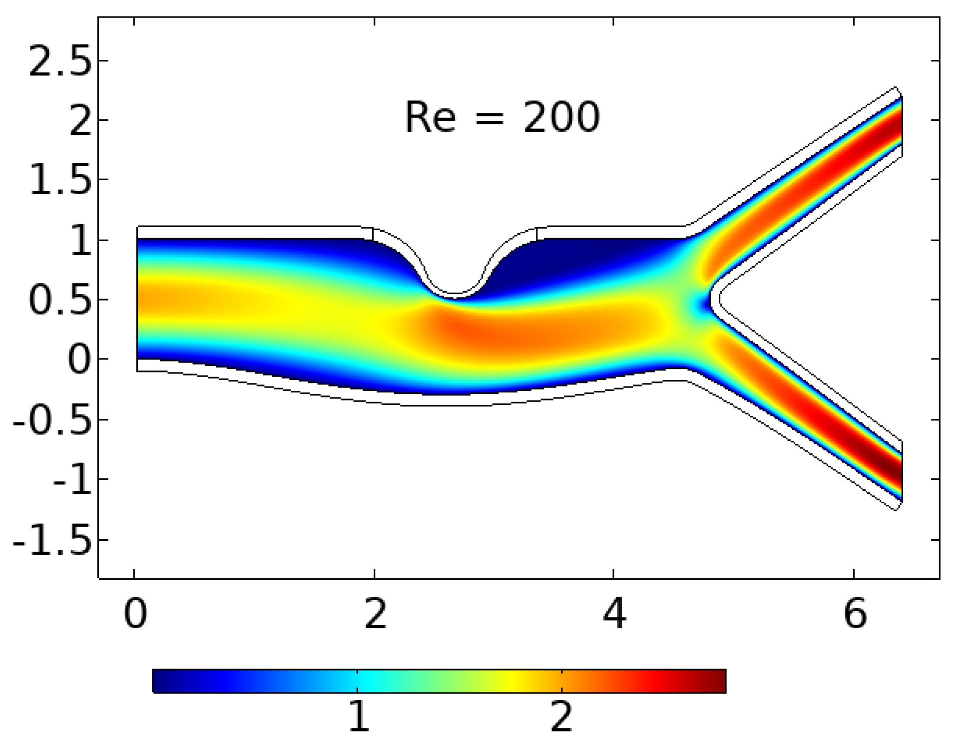
6.1. Velocity Profile

Figure 3 displays the blood flow behavior at $Re=200$ nonturbulent flow. As observed, the blood flow velocity decreased by $26\%$, from about 2.3 units to 1.7 units, as it approached the stenotic region labeled ‘B’. The gradual increase in the arterial diameter by approximately $31.5\%$ at the beginning part of the stenotic region is the cause of this drop in velocity. Moreover, the lower wall of the artery expanded more than the upper wall due to its Young’s modulus being around $25\%$ less than the upper wall, which is more rigid because of the plaque’s inherent property. The decrease in blood velocity in the expanded lower wall caused a region of relatively high pressure normal to the wall surface, resulting in arterial wall expansion.

Figure 3. Velocity contour maps with Reynolds number $Re=200$.

It is worth noting that backflow nucleation occurred at the bifurcation point as the blood divided into branches with smaller diameters, causing an increase in velocity compared to the main artery by around $30\%$. These findings provide insight into the effects of stenosis on blood flow behavior and arterial wall expansion. The results also highlight the significance of considering the heterogeneous properties of arterial walls when analyzing blood flow behavior in stenotic arteries.

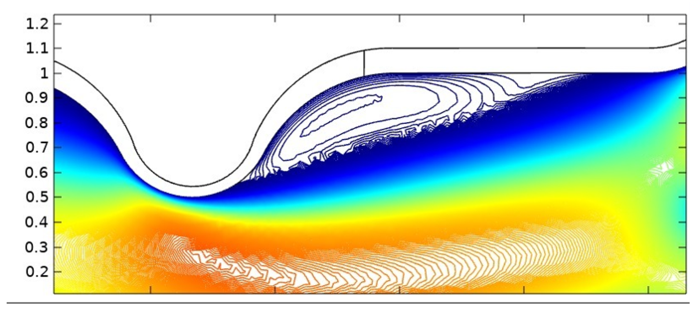
6.2. Blood Backflow

The velocity vector simulation results of blood flow at Reynolds number $Re=200$ are presented in Figure 4. The left image shows the normalized velocity vectors of the blood flow as it moves across the artery, revealing significant backflow in the trailing edge of the plaque, even at a low Reynolds number. However, it is not evident from this image whether there is any stagnation or other irregularity in the blood flow patterns. A low-velocity values, high-pressure effects are showcased in Figure 5.

Figure 4. Normalized and actual velocity vector results showing blood backflow in the trailing end of the plaque.

Figure 5. Low-velocity–high-pressure effect causing the arterial wall to expand.

The right image in Figure 4 shows the actual velocity of the blood flow, which is indicated by the length of the arrows. It is apparent from this image that the relative velocity of blood in the trailing edge of the plaque is much lower, by over $90\%$. This low flow rate can result in blood stagnation and the formation of micro-vortices, which can lead to activation and stress on blood platelets, further exacerbating the process of atherosclerosis. Such changes in the flow pattern of the blood flow can increase the likelihood of blood particle deposition at the stenosis region and subsequent thrombosis.

6.3. Higher Reynolds Number

Figure 6 shows the lower wall deformation for a Reynolds number of $Re=2000$, which is relatively small due to the high velocity and low normal pressure. As the Reynolds number increased from $Re=200$ to 2000, the effects of backflow, stagnation, vortices, and low lateral velocities were further amplified, as expected. Figure 6 and Figure 7 illustrate these effects.

Figure 6. $Re=2000$ lower wall deformation is very small due to high velocity and low normal pressure.

Figure 7. With $Re=2000$, the stagnation region grew significantly.

Moreover, as the velocity of the blood flow increased, the normal pressure on the arterial wall decreased. This resulted in a small deformation of the arterial wall, which is apparent when comparing Figure 3 with Figure 6 and Figure 7.

Figure 7 also shows that the stagnation region grew significantly with a Reynolds number of $Re=2000$.

6.4. Dynamic Energized Hotspots

At the backflow region labeled ‘H’ in Figure 8, the blood flow characteristics can create an environment conducive to the formation of highly Dynamic Energized Hot Spots (DEHSs).

Figure 8. Higher magnified region of the trailing end of the artery where there is significant backflow.

DEHSs are micro- to mini-sized vortices with low lateral speed (stagnation) but high rotational inertia. The vortices increase both the normal and shear stress in this region, causing further lesions to the plaque. This, in turn, activates the platelets and recruits more blood cells to the plaque, causing it to grow larger. Due to the low lateral speed, the damage to the artery wall and plaque can be severe. If these DEHSs are frequently in contact with a vulnerable region of the plaque, it can cause it to rupture, leading to thrombosis.

The severity of the damage caused by DEHSs emphasizes the need to understand the dynamics of blood flow and the associated fluid mechanics in atherosclerotic arteries. Figure 8 provides a higher magnified view of the trailing end of the artery where there is significant backflow, which can serve as a breeding ground for the formation of DEHSs.

6.5. Shear Stress

The slight narrowing of the arterial wall in the stenotic region caused the blood velocity to increase as the blood flow moved across the region. Figure 3 shows that the average velocity changes from high (2.2) to low (1.6) and then high (2.5) as the blood flowed across the artery. It is worth noting that the high-velocity resulted in greater shear stress at the plaque region. Specifically, as the blood flowed at its highest velocity through the narrowest region or the cap of the plaque, the shear stress was the greatest, as depicted in Figure 9.

Figure 9. High shear stress can result in the fracture of the cap of the plaque.

The high shear stress can cause the fracture of the plaque cap, leading to thrombus formation and even to myocardial infarction. Understanding the effects of shear stress on plaque vulnerability is essential to prevent and manage atherosclerosis-related complications. Figure 9 highlights the importance of assessing and monitoring shear stress levels in patients with stenotic plaques.

6.6. Wall Shear Stress

Observing wall shear stress (WSS) is essential to reduce the recirculation area in stenosed arteries, which in turn can lower the risk of atherosclerosis. Figure 10 illustrates the behavior of WSS in the stenosis for different Reynolds numbers ($Re$). The figure shows that as $Re$ decreased, the magnitude of WSS increased. This indicates that a decrease in $Re$ can reduce the chance of atherosclerosis in the stenosed region by increasing the total WSS experienced by the stenosis. Furthermore, it has been observed that WSS can play a crucial role in the formation and development of atherosclerotic plaques. A low or disturbed WSS can cause the endothelium to become dysfunctional and lead to the initiation of atherosclerosis. On the other hand, a high and unidirectional WSS can maintain the endothelium in a healthy state and protect against atherosclerosis. Therefore, the measurement and analysis of the WSS can provide valuable insights into the progression and treatment of cardiovascular diseases.

Figure 10. Total wall shear stress experienced by the stenosis from A to B.

6.7. Wall Displacement

The deformation of the arterial wall is an important factor to consider, as it can affect the overall health of the artery. In Figure 11, the behavior of wall displacement is shown. It can be observed that there is a comparatively small deformation at the stenosis position. This is due to the difference in elastic modulus between the stenotic and nonstenotic walls. As the value of Reynolds number $Re$ increased, the displacement or deformation of the wall decreased.

Figure 11. Total displacement of the upper wall.

It is important to note that excessive deformation of the arterial wall can lead to the rupture of the plaque and cause further damage to the artery. Therefore, monitoring the wall displacement can provide insight into the overall health of the artery and can be used as an early warning sign for potential health problems. Further research is needed to determine the optimal range of wall displacement for healthy arterial function.

7. Summary and Conclusions

In summary, the behavior of blood flow in a stenosed artery can have significant impacts on the development and progression of atherosclerosis. High shear stress and wall displacement are key factors to observe when analyzing the behavior of blood flow. Shear stress, caused by the high velocity of blood flow in the narrowest region or the cap of the plaque, can result in the fracture of the cap of the plaque, leading to thrombosis. Wall displacement or deformation, caused by the different elastic modulus at the stenosis and the other wall, can reduce as the value of the Reynolds number increases. Wall shear stress is another important factor to observe, as it helps to reduce the recirculation area in a stenosed artery. The magnitude of the WSS increases with a decrease in Reynolds number, which in turn, reduces the chance of atherosclerosis.

The computer model and simulation results have demonstrated a notable alteration in the blood flow dynamics as blood moves through the stenotic region of the artery. The observed changes encompass the expansion of the arterial wall, modifications in the velocity profiles, and the presence of blood stagnation and backflow. Based on the obtained results, it has been suggested that highly dynamic energized hot spots (DEHSs) may form, and this can lead to the development of a larger plaque, which can further narrow the artery lumen. Moreover, the simulation results have also revealed that the high shear stress at the narrowest part of the artery, which is located at the cap of the plaque, may cause it to rupture.

In conclusion, a better understanding of the behavior of blood flow in a stenosed artery can aid in the prevention and treatment of atherosclerosis. Factors such as shear stress and wall displacement should be considered when analyzing the risk of atherosclerosis in a patient. Future research could focus on developing more accurate and comprehensive models of blood flow behavior in a stenosed artery, as well as investigating new methods for preventing and treating atherosclerosis.