Control Law for Two-Process Flexible Manufacturing Systems Modeled Using Petri Nets

Abstract

The deadlock control problem in flexible manufacturing systems (FMSs) has received much attention in recent years. The formalism of the Petri net is employed to effectively model, analyze, and control deadlocks in an FMS case study. There are many kinds of deadlock prevention strategies based on the Petri net approach, where computational complexity is a major problem that needs to be considered. Based on the Petri net theory, this paper focuses on the two special subclasses in the ${\mathrm{S}}^3$PR net, namely the dual-process ${\mathrm{S}}^3$PR and the dual-process ${\mathrm{US}}^3$PR, in a bid to prevent deadlocks in an FMS. The relationship between the net structural characteristics and the deadlocks reached was analyzed, and then a regular method of adding controllers for these two models was proposed to reduce computational complexity.

1. Introduction

In flexible manufacturing systems (FMSs) [1,2], a resource is usually shared by different processes. If the resource allocation is not appropriate, the system may move to deadlocks [3], where any deadlock makes the whole system or part of the system unable to be operated, and indirectly causes incalculable economic losses or other catastrophic consequences. Therefore, a deadlock is a situation that FMSs should avoid. The description, analysis, solution, and control of deadlocks in FMSs are undoubtedly of vital importance to ensure the normal operation of the system.

The Petri net theory [4,5] has a strict mathematical expression and intuitive graphical expression, and is often used for the modeling, deadlock analysis, and control of FMSs. In the Petri net theory, there mainly exist three approaches for solving the deadlock problem: deadlock detection and recovery [6], deadlock avoidance [7,8], and deadlock prevention [9,10,11]. The reachability graph analysis method [12,13,14] is a fundamental technique for deadlock prevention, which provides complete and detailed information about the dynamic behavior of Petri nets since all-state place enumeration is considered. Moreover, the structural analysis method [15,16,17,18] is marking-independent and only depends on the place–transition relationship of the underlying net by the flow relation. Uzam and Zhou [19] proposed an active controller design method using the iterative method. The proposed method simplifies the calculation of the control places, but it cannot guarantee optimal controllability and solves the reachability graph repeatedly. In addition, Chen et al. [20] propose another iterative controller design method, which has higher computational efficiency and achieves optimal control. In the proposed method, first, the minimum cover sets of legal and first-time damaged identifiers are obtained by vector coverage. Second, by solving an integer linear programming problem, a P-invariant is designed to prevent the system from reaching the first-time damaged identifier, and then the illegal identifier is forbidden. Finally, the optimal controller of the system is obtained.

Siphons are closely related to deadlock on structural analysis [21]. Once a siphon is emptied, all transitions related to the siphon in the net become dead, and then the system is blocked. Therefore, siphon control is a typical deadlock prevention strategy based on structure analysis. Ezpeleta et al. [22] define the system of simple sequential processes with resources (${\mathrm{S}}^3$PR), and propose a controller design method for adding control places to all strict minimal siphons to avoid the result that siphons become emptied. The proposed method realizes the active control of the net but, for the large-scale net, a large number of control places need to be added, which makes the net structure extremely complex. Huang et al. [23] propose an iterative deadlock control strategy based on ${\mathrm{S}}^3$PR, where the strategy is divided into two stages. One is siphon control, and the other is control-induced siphon control. To reduce the complexity of the model structure, Li et al. [24] propose the concepts of the basic siphon and subordinate siphon, proving that the controllability of the subordinate siphon can be guaranteed by the controllability of the basic siphon if the basic siphon is controlled under certain conditions. Additionally, they propose the method of adding controllers to basic siphons as controlled places, which reduces the scope of controlled places, the computational complexity, and structural complexity, and is more suitable for large-scale Petri nets, compared with the method proposed in [22]. In addition to adding control places from the siphon point of view, Xing et al. [25] utilize the resource transition (RT) circuits of ${\mathrm{S}}^3$PR to describe the deadlock of the system, where a deadlock state occurs if a maximal perfect RT-circuit (MPRTC) is saturated, and a controller is designed to retain the maximally permissive behavior of ${\mathrm{S}}^3$PR without $\xi$ resources. However, the method has to face the problems of computational complexity and structural complexity. Liu et al. [26] put forward the concept of transition coverage, and prove that an active Petri net controller can be obtained only by controlling the maximal perfect RT-circuit under change coverage. As a result, the proposed method reduces the computational complexity of controlling and structural complexity of the net.

This paper studies dual-process ${\mathrm{S}}^3$PR and dual-process ${\mathrm{US}}^3$PR and analyzes the relationship between their structural characteristics and deadlock, where the control places are added to form the P-invariant with the activity places in the original net to realize deadlock prevention. The relationship between the control places and the net size is that the two special subclasses have fixed control laws. For a given dual-process ${\mathrm{S}}^3$PR and a dual-process ${\mathrm{US}}^3$PR, there is no need for the complex calculation of siphons or RTC, since control places can be directly added to the net to ensure that the system is alive.

The contributions of the paper are twofold as follows.

• This study introduces the concept of encounter place pair and encounter state in the dual-process ${\mathrm{S}}^3$PR, and the relationship between the encounter state and deadlock is analyzed. When the initial marking of the resource place is 1, the addition of control places prevents the occurrence of encounter states, progressive encounter states, and blocked states, ensuring that the net is live and maximally permissive. Moreover, the control law of dual-process ${\mathrm{S}}^3$PR is summarized.
• This paper utilizes the concept of ${\mathrm{US}}^3$PR and analyzes the relationship between a saturated pair of encounter paths and deadlock in dual-process ${\mathrm{US}}^3$PR. As a result, the optimal active-controlled system is obtained by adding control places. The mathematical relationship between the number of independent resource holder loops and the number of control places in the dual-process ${\mathrm{US}}^3$PR is analyzed, and the control law of the dual-process ${\mathrm{US}}^3$PR is obtained indirectly.

2. Preliminaries

2.1. Petri Nets

A Petri net (PN) is a four-tuple $N=(P,T,F,W)$, where P and T are non-empty and finite sets of elements named places and transitions, and $P\cap T=\varnothing$. F is a flow relation set of a PN, where $F\subseteq (P\times T)\cup (T\times P)$ is represented by directed arcs pointing from transitions to places (or places to transitions). Let $\mathbb{N}$ denote the set of non-negative integers. W:$F\to \mathbb{N}$ represents a map that assigns a non-negative integer number (weight) to each arc in F, i.e., $W(i,j)>0$ if $(i,j)\in F$, else $W(i,j)=0$. A PN $N=(P,T,F,W)$ is ordinary, if, for all $(i,j)\in F$, $W(i,j)=1$.

M is a marking of a PN, which is a map: $P\to \mathbb{N}$. For a place $p\subseteq P$, $M\left(p\right)$ represents the quantity of tokens in it. A place p is marked, if $M\left(p\right)>0$. A subset $P_s\subseteq P$ is marked if there exists at least one place $p\subseteq P_s$ marked by M. $M\left(P_s\right)={\sum }_{p\in S}M\left(p\right)$. $(N,M_0)$ is said to be a marked net with $M_0$ being called an initial marking.

Let $i\in P\cup T$ be an element of a PN $N=(P,T,F,W)$. ${}^{•}i=\{j\in P\cup T\mid (j,i)\in F\}$ is the preset of i; $i^{•}=\{j\in P\cup T\mid (i,j)\in F\}$ is the the postset of i. The previous notation is extended to sets of nodes; if $I\subseteq P\cup T$, ${}^{•}I={\cup }_{i\in I}{}^{•}i$, then $I^{•}$ = ${\cup }_{i\in I}$$i^{•}$. If, for all $x\in \{1,2,\dots ,n-1\}:i_{x+1}\in i_x^{•}$, a path $i_1\cdots i_n$ of N is defined as a string $i_1,\dots ,i_n$, where $\forall i\in \{i_1,\dots ,i_n\}$, $i\in P\cup T$. A path $i_1\cdots i_n$ is an elementary path, if all nodes of it are different (except, perhaps, $i_1$ and $i_n$). A path $i_1\cdots i_n$ is a circuit if it is an elementary path and $i_1=i_n$.

A transition $t\in T$ is enabled at a marking M if, for all $p\in {}^{•}t$, $M\left(p\right)\ge W(p,t)$, which is denoted by $M[t\rangle$. Firing t to a new marking $M^{\prime }$ such that for all $p\in P$, $M^{\prime }\left(p\right)=M\left(p\right)-W(p,t)+W(t,p)$, denoted by $M[t\rangle M^{\prime }$. If there is a sequence of transitions $\sigma$ = $t_0{t}_1\dots t_n$ as well as markings $M_1,M_2\dots M_n$, such that $M[t_0\rangle M_1[t_1\rangle M_2\dots M_n[t_n\rangle M^{″}$ holds, we can say $M^{″}$ is reachable from marking M. $R(N,M)$ is called the reachability set which denotes all the markings reachable from M in $(N,M)$. A reachability graph of a net is denoted as $RG$. A PN $N=(P,T,F,W)$ is called a state machine if, for all $t\in T$, ${|}^{•}t|=|t^{•}|=1$.

A net $N=(P,T,F,W)$ is pure if, for all $x,y\in P\cup T$, $W(x,y)>0$ implies $W(y,x)=0$. It can be noticed that a pure PN $N=(P,T,F,W)$ is able to be represented by an incidence matrix $\left[N\right]$, where $\left[N\right](p,t)=W(t,p)-W(p,t)$. This incidence matrix $\left[N\right]$ can be divided into two parts: $\left[N\right]=$ Post−Pre, where Post$(p,t)=W(t,p)$ and Pre$(p,t)=W(p,t)$ are called the output matrix and input matrix, respectively.

Given a PN ($N,M_0$), $t\in T$ is live under $M_0$ if $\forall M\in R(N,M_0),\exists M^{\prime }\in R(N,M),$ $M^{\prime }$$[t\rangle$. $(N,M_0)$ is live if $\forall t\in T$, t is live under $M_0$. $(N,M_0)$ is dead under $M_0$ if $\nexists t\in T$, $M_0$$[t\rangle$.

A P-vector is a column vector $I:P\to \mathbb{Z}$ indexed by P, where $\mathbb{Z}$ is the set of integers. The P-vector I is called a P-invariant (place invariant) if $I\ne 0$ and $I^T\left[N\right]={\mathbf{0}}^T$. The P-invariant I is a P-semiflow if every element of I is non-negative. $\parallel I\parallel =\left\{p\in P\left|I\right(p)\ne 0\right\}$ is called the support of I.

Let S be a non-empty subset of places. S is called a siphon (trap) if ${}^{•}S\subseteq S^{•}(S^{•}\subseteq {}^{•}S)$ holds. A siphon is said to be minimal if there is no siphon contained in it as a proper set. A minimal siphon is said to be strict if it does not contain a trap. A strict minimal siphon is denoted as SMS for short. $\mathsf{\Pi }$ denotes the set of SMSs in a PN.

2.2. $S^3$PR

The system considered can be modeled as a system of simple sequential processes with resources (${\mathrm{S}}^3$PR) if there is no unreliable resource. The definition of ${\mathrm{S}}^3$PR is briefly introduced as follows.

Definition 1

([22]). Let $(N_1,M_1)$ and $(N_2,M_2)$ be PNs with $N_1=(P_1,T_1,F_1,W_1)$ and $N_2=(P_2,T_2,F_2,W_2)$, where $P_1\cap P_2=P_C\ne \varnothing$ and $T_1\cap T_2=\varnothing$. The net $(N,M)$ with $N=(P,T,F,W)$ is said to be the resultant of composing $(N_1,M_1)$ and $(N_2,M_2)$ via the set of shared places $P_C$ if (1) $P=P_1\cup P_2$, $T=T_1\cup T_2$, $F=F_1\cup F_2$, and $W(x,y)=W_i(x,y)$ if $(x,y)\in F_i$, $i=1,2$; and (2) $\forall p\in P_1\setminus P_C$, $M\left(p\right)=M_1\left(p\right)$, $\forall p\in P_2\setminus P_C$, $M\left(p\right)=M_2\left(p\right)$, and $\forall p\in P_C$, $M\left(p\right)=max\{M_1\left(p\right),M_2\left(p\right)\}$. The composition of $N_1$ and $N_2$ is denoted by $N_1⨂N_2$.

Definition 2

([22]). A system of simple sequential processes with resources ($S^3$PR) is the PN $N={◯}_{i=1}^n{N}_i=(P_A,\left\{p^0\right\},P_R,T,F)$ defined as the union of a set of nets $N_i=(P_{A_i},\left\{p_i^0\right\},P_{R_i};T_i;F_i)$ sharing common places, where the following statements are true:

• $p_i^0$ is called the process idle place of $N_i$. Elements in $P_{A_i}$ and $P_{R_i}$ are called activity or operation and resource places, respectively. A resource place is called a resource for short in case of no confusion.
• $P_{R_i}\ne \varnothing ;P_{A_i}\ne \varnothing ;\left\{p_i^0\right\}\notin P_{A_i};(P_{A_i}\cup \left\{p_i^0\right\})\cap P_{R_i}=\varnothing ;\forall p\in P_{A_i},\forall t\in {}^{•}p,\forall t^{\prime }\in p^{•},\exists r_p\in P_{R_i},{}^{•}t\cap P_{R_i}=t^{\prime •}\cap P_{R_i}=\left\{r_p\right\};\forall r\in P_{R_i},{}^{••}r\cap P_{A_i}=r^{••}\cap P_{A_i}\ne \varnothing ;\forall r\in P_{R_i},{}^{•}r\cap r^{•}=\varnothing$; and ${}^{••}\left\{p_i^0\right\}\cap P_{R_i}=\varnothing$.
• ${\overline{N}}_i$ is a strongly connected state machine, where $\overline{N_i}=(P_{A_i},\left\{p_i^0\right\},P_{R_i};T_i;F_i^{\prime })$ is the resulting net after the places in $P_{R_i}$ and related arcs are removed from $N_i$ and $F_i^{\prime }=F_i\cap \{[(P_{A_i}\cup \left\{p_i^0\right\})\times T_i]\cup [T_i\times (P_{A_i}\cup \left\{p_i^0\right\})]\}$.
• Every circuit of $\overline{N_i}$ contains place $p_i^0$.
• Any two $\overline{N_i}$ s are composable when they share a set of common places. Every shared place must be a resource.
• Transitions in ${}^{•}\left\{p_i^0\right\}$ and ${\left\{p_i^0\right\}}^{•}$ are called the source and sink transitions of an $S^3$PR, respectively.

Definition 3

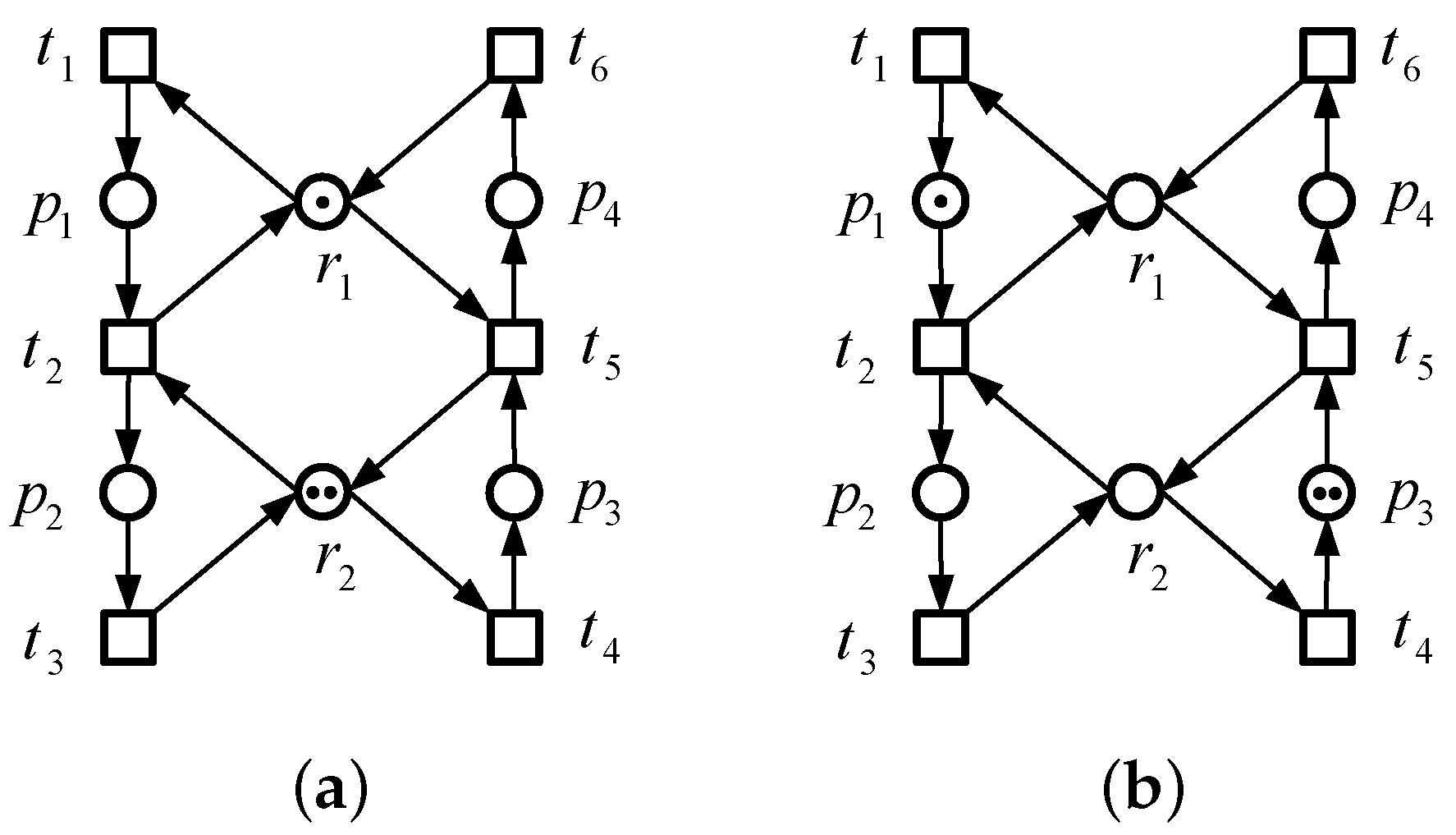
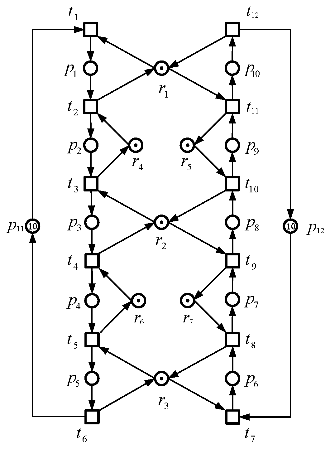
([22]). A PN $N=(P_A\cup \left\{p^0\right\}\cup P_R,T,F)$ is an $S^3$PR and let S be an SMS in N. $S_R=S\cap P_R$ and $S_A=S\setminus S_R$ represent the set of resource places and the set of activity places in S, respectively. For $r\in P_R$, $H\left(r\right){=}^{••}r\cap P_A$ is called the set of holders of r, which means that these activity places in $H\left(r\right)$ need resource r. Let $\left[S\right]={\cup }_{r\in S_R}H\left(r\right)\setminus S$ and it is called the complementary set of siphon S.

Figure 1 is an ${\mathrm{S}}^3$PR that has eleven places and eight transitions, where $\left\{p_1^0\right\}=\left\{p_1\right\},\left\{p_2^0\right\}=\left\{p_5\right\}$, $P_{A_1}=\{p_2,p_3,p_4\}{P}_{A_2}=\{p_6,p_7,p_8\}$, and $P_R=\{p_9,p_{10},p_{11}\}$. The sets $S_1=\{p_3,p_8,p_9,p_{10}\}$, $S_2=\{p_4,p_7,p_{10},p_{11}\}$, and $S_3=\{p_4,p_8,p_9,p_{10},p_{11}\}$ are three SMSs for the PN. According to Definition 3, we have $H\left(r_1\right)=\{p_2,p_8\}$, $H\left(r_2\right)=\{p_3,p_7\}$, and $H\left(r_3\right)=\{p_4,p_6\}$, which means that places $p_2$ and $p_8$ can use resources in $r_1$, $p_3$ and $p_7$ can use resources in $r_2$, and resources in $r_3$ can be used by places $p_4$ and $p_6$. Their complementary sets are $\left[S_1\right]=\{p_2,p_7\}$, $\left[S_2\right]=\{p_3,p_6\}$, and $\left[S_3\right]=\{p_2,p_3,p_6,p_7\}$, respectively.

Definition 4

([22]). Let $N=(P_A\cup \left\{p^0\right\}\cup P_R,T,F)$ be an $S^3$PR, and x and y are two different nodes in $P_A\cup T$. (1) A path in N that merely contains activity places in $P_A$ and transitions in T is called an operation path. (2) If there exists an operation path in N from x to y, it is said that x is previous to y in N, which is denoted as $x{<}_{N}y$. (3) Let $A\subseteq (P_A\cup T)$. If there is a node $y\in A$ with $x{<}_{N}y$, we can obtain $x{<}_{N}A$. If there exists a node $y\in A$ such that $y<{}_{N}x$, then $A<{}_{N}x$.

Let us consider the net shown in Figure 1, where $p_1{t}_1{p}_2{t}_2{p}_3{t}_3{p}_4{t}_4{p}_1$ is a circuit and $p_2{t}_2{p}_3{t}_3$ is a path in this circuit. Clearly, we have $p_2<{}_N{p}_3$.

3. Control Law for Dual-Process ${\mathbf{S}}^{\mathbf{3}}$PR

In the Petri net-based deadlock prevention strategy, computational complexity is a problem that needs to be faced. This section proposes a regular method by adding control places for the dual-process ${\mathrm{S}}^3$PR model, which avoids the calculation of siphons or reachable graphs. First, the concept of the dual-process ${\mathrm{S}}^3$PR and its encounter state are introduced. Then, the activity analysis of this special model is carried out, and the activity of the model is guaranteed by adding the control places, and then the control law of such model is obtained.

3.1. Dual-Process $S^3$PR and Encounter State

Definition 5.

Let $N=(P_A\cup P^0\cup P_R,T,F)$ be a normal $S^3$PR; it is called a dual-process $S^3$PR if

• $|P^0|=2$;
• $|P_{A1}|=|P_{A2}|=|P_R|$;
• $\forall p\in P_A\cup P^0$, $|{}^{•}p|=|p^{•}|=1$;
• (a) ${p_1^0}^{••}\cap P_A=\left\{p\right\}$,${}^{••}{p}_2^0\cap P_A=\left\{p^{\prime }\right\}$, ${}^{••}p\cap P_R={}^{••}{p}^{\prime }\cap P_R\ne \varnothing$; (b) $p_1\in P_{A1}$, $p_2\in P_{A2}$, ${p_1}^{••}\cap P_A=\left\{p_1^{\prime }\right\}$, ${}^{••}{p}_2\cap P_A=\left\{p_2^{\prime }\right\}$; if ${}^{••}{p}_1\cap P_R={}^{••}{p}_2\cap P_R\ne \varnothing$, so ${}^{••}{p}_1^{\prime }\cap P_R={}^{••}{p}_2^{\prime }\cap P_R\ne \varnothing$.

Given a dual-process ${\mathrm{S}}^3$PR net, the subscripts of places and transitions are arbitrary but, for the convenience of description, they need to be initialized in this chapter. Based on the definition in the previous section, Algorithm 1 is proposed to formalize the subscript initialization method for a dual-process ${\mathrm{S}}^3$PR, where Line 1 defines the output $N=(P_A\cup P^0\cup P_R,T,F)$. According to the rules, all places p and transitions t are numbered in Lines 2–24. The flow relations f remain unchanged in Lines 25–27. When the number of the resource places is $n(n\in {\mathbb{N}}^{+})$:$P^0=\left\{p_1\right\}\cup \left\{p_{n+2}\right\}$, $P_{A1}=\{p_2,p_3,\cdots ,p_{n+1}\}$, $P_{A2}=\{p_{n+3},p_{n+4},\cdots ,p_{2n+2}\}$, $P_R=\{r_1,r_2,\cdots ,r_n\}$, $T=\{t_1,t_2,\cdots ,t_{2n+2}\}$. In addition, $p_1^0$ corresponds to circuit $C_1=p_1{t}_1{p}_2{t}_2{p}_3···t_n{p}_{n+1}{t}_{n+1}{p}_1$ and $p_2^0$ corresponds to circuit $C_2=p_{n+2}{t}_{n+2}{p}_{n+3}{t}_{n+3}{p}_{n+3}···t_{2n+1}{p}_{2n+2}{t}_{2n+2}{p}_{n+2}$, where $C_1$ and $C_2$ represent process 1 and process 2, respectively. When a token is fired from the idle place and then returns to the idle place through the circuit $C_1$ or $C_2$, the process ends normally. For instance, Figure 2 displays a subscript-initialized dual-process ${\mathrm{S}}^3$PR.

Definition 6.

Let $x_1{x}_2···x_n$ be an elementary process path in a dual-process $S^3$PR; $T_{x_1-x_n}=\left\{y\right|y\in \{x_1,x_2,···,x_n\}\cap T\}$ is said to be the transition set from $x_1$ to $x_n$; $P_{x_1-x_n}=\left\{y\right|y\in \{x_1,x_2,···,x_n\}\cap P\}$ is said to be the place set from $x_1$ to $x_n$.

Algorithm 1: The subscript initialization method for a dual-process ${\mathrm{S}}^3$PR

Definition 7.

Let $N=(P_A\cup P^0\cup P_R,T,F)$ be a dual-process $S^3$PR; $\exists \{r,r^{\prime }\}\in P_R$, $\exists \{t,t^{\prime }\}\in T$; ordered pair ${\varphi }_r=(r,r^{\prime })$ is said to be an adjacent resource place pair and ordered pair ${\varphi }_{mt}=(t,t^{\prime })$ is said to be an encounter transition pair if $({}^{•}r\cap {r^{\prime }}^{•})\cap T_1=\left\{t\right\}$ and $(r^{•}\cap {}^{•}{r}^{\prime })\cap T_2=\left\{t^{\prime }\right\}$; ordered pair ${\varphi }_{mp}=(p,p^{\prime })$ is said to be an encounter place pair if ${}^{•}t\cap P_A=\left\{p\right\}$ and ${}^{•}{t}^{\prime }\cap P_A=\left\{p^{\prime }\right\}$.

According to Definitions 2 and 5, in a dual-process ${\mathrm{S}}^3$PR net, for $\forall t\in T$, firing t will consume one token of $r\in P_R$ and, if $t\in T_1\setminus \{{p_1^0}^{•}\cup {}^{•}{p}_1^0\}$ and $t^{\prime }\in T_2\setminus \{{p_2^0}^{•}\cup {}^{•}{p}_2^0\}$, firing t will consume one token of $r^{\prime }$ and release one token of r. So, the intersections $({}^{•}r\cap {r^{\prime }}^{•})\cap T_1=\left\{t\right\}$ and $(r^{•}\cap {}^{•}{r}^{\prime })\cap T_2=\left\{t^{\prime }\right\}$ are not empty.

Definition 8.

Let $(N,M_0)=(P_A\cup P^0\cup P_R,T,F,M_0)$ be a marked dual-process $S^3$PR, ${\varphi }_r$ be an adjacent resource place pair in N, ${\varphi }_{mp}$ be an encounter place pair associated with ${\varphi }_r$, and $M\in R(N,M_0)$; M is said to be an encounter state marking if $M\left({\varphi }_{mp}\right)=M_0\left({\varphi }_r\right)$, noted as $M_e$.

A dual-process ${\mathrm{S}}^3$PR net removes the idle places and the associated directed arcs; the subnet shown in Figure 3, $({}^{•}{r}_1\cap {r_2}^{•})\cap T_1=\left\{t_2\right\}$, $({r_1}^{•}\cap {}^{•}{r}_2)\cap T_2=\left\{t_5\right\}$. ${\varphi }_r=(r_1,r_2)$ is the adjacent resource place pair; ${\varphi }_{mt}=(t_2,t_5)$ is the encounter transition pair. ${}^{•}{t}_2\cap P_A=\left\{p_1\right\}$, ${}^{•}{t}_5\cap P_A=\left\{p_3\right\}$, so the encounter place pair is ${\varphi }_{mp}=(p_1,p_3)$.

Figure 3a shows the subnet with non-encounter state marking, where $M\left({\varphi }_{mp}\right)=M\left(p_1\right)+M\left(p_3\right)=0$, $M\left({\varphi }_{mp}\right)\ne M_0\left({\varphi }_r\right)$; the encounter place pair does not occupy the token in the associated adjacent resource place pair. Figure 3b shows the subnet with encounter state marking, where $M\left({\varphi }_{mp}\right)=M\left(p_1\right)+M\left(p_3\right)=M_0\left(r_1\right)+M_0\left(r_2\right)=M_0\left({\varphi }_r\right)$; the encounter place pair occupies all the tokens in the adjacent resource place pair associated with it.

Theorem 1.

Given a marked dual-process $S^3$PR $(N,M_0)$, if $M_e\in R(N,M_0)$, then deadlocks will occur in it.

Proof. 

According to Definition 5, in the case of ${\varphi }_{mt}=(t,t^{\prime })$, firing t will consume one token of $r^{\prime }$ and release one token of r. Similarly, firing $t^{\prime }$ will consume one token of r and release one token of $r^{\prime }$. If M is an encounter state marking, $M\left({\varphi }_{mp}\right)=M_0\left({\varphi }_r\right)$, $M\left(r\right)=M\left(r^{\prime }\right)=0$, the places of the encounter place pair occupy all tokens in the adjacent resource place pair associated with it. Thus, both t and $t^{\prime }$ cannot fire, and deadlocks occur in the ${\mathrm{dual-process S}}^3$PR.    □

Figure 4a shows a dual-process ${\mathrm{S}}^3$PR with encounter state marking $M_e$. For adjacent resource place pair ${\varphi }_r=(r_2,r_3)$, ${\varphi }_{mp}=(p_3,p_8)$ is the encounter place pair associated with it; $M\left(p_3\right)=M_0\left(r_2\right)=1$, $M\left(p_8\right)=M_0\left(r_3\right)=1$, and $M\left(r_2\right)=M\left(r_3\right)=0$, ${\varphi }_{mp}=(p_3,p_8)$ occupy all tokens in ${\varphi }_r=(r_2,r_3)$, so $t_5$ and $t_8$ cannot be fired; thus, $r_2$ and $r_3$ cannot obtain the tokens again, and $t_2$ and $t_7$ cannot be fired similarly, forming a circular wait. In other words, a deadlocks occur in this net. But $t_1$ is enabled in circuit $C_1$, and $t_6$ is enabled in circuit $C_2$, so the net is not dead. If $t_1$ and $t_6$ are fired, all resource places in the net have no tokens, all transitions cannot be fired, and it means the net is dead, as shown in Figure 4b.

3.2. Control Law for Dual-Process $S^3$PR with $M_0\left(r\right)$ Equals to 1

Definition 9.

Given a marked dual-process $S^3$PR $(N,M_0)=(P_A\cup P^0\cup P_R,T,F,M_0)$, where $(\forall r\in P_R)M_0\left(r\right)=1$, let ${\varphi }_{mp}=(p_i,p_j)$ be an encounter place pair of N. The order pair ${\varphi }_{lp}=(p,p^{\prime })$ is said to be a progressive encounter place pair if ${\varphi }_{lp}\ne {\varphi }_{mp}$, where $p\in P_{p_2-p_i},p^{\prime }\in P_{p_{n+3}-p_j}$, and ${\mathsf{\Phi }}_{lp}$ denotes the set of all progressive encounter place pairs of N.

Definition 10.

Let $(N,M_0)=(P_A\cup P^0\cup P_R,T,F,M_0)$ be a marked dual-process $S^3$PR, where $(\forall r\in P_R)M_0\left(r\right)=1$. Assume that ${\varphi }_{lp}=(p,p^{\prime })$ is a progressive encounter place pair; then, $M\in R(N,M_0)$ is a progressive encounter state marking if $M\left(p\right)=M\left(p^{\prime }\right)=1$, noted as $M_{pe}$.

Theorem 2.

Given a marked dual-process $S^3$PR $(N,M_0)=(P_A\cup P^0\cup P_R,T,F,M_0)$, where $(\forall r\in P_R)M_0\left(r\right)=1$, and $M_{pe}\in R(N,M_0)$, then there is a sequence of transitions σ, satisfying $M_{pe}[\sigma \rangle M_e$.

Proof. 

In the marked dual-process ${\mathrm{S}}^3$PR $(N,M_0)$, if $M_0[{\sigma }^{\prime }\rangle M_{pe}$, it means that both processes 1 and 2 have artifacts entering the system. Since the initial marking of every resource place is 1, and the order of use of resources by processes 1 and 2 is reversed, if there are workpieces in both processes, then, after a certain transition sequence is transmitted, the two workpieces will inevitably enter the encounter places, denoted by $M_{pe}[\sigma \rangle M_e$.    □

As shown in Figure 5a, the place pair $(r_1,r_2)$ is an adjacent resource place pair and $(p_2,p_9)$ is an encounter place pair associated with it, $(p_2,p_8)$ is a progressive encounter place pair according to Definition 9, and $M\left(p_2\right)=M\left(p_8\right)=1$ is a progressive encounter state marking according to Definition 10. The transitions $t_2,t_6,t_8$ can be fired at this moment. When $t_8$ is fired, $M\left(p_2\right)=M\left(p_9\right)=1$ is an encounter state marking, which is shown in Figure 5b. The transitions $t_1,t_2,t_3,t_4,t_5,t_7,t_8,t_9,t_{10}$ cannot be fired; only $t_6$ can be fired at this moment. Then, firing a sequence of transitions $\sigma =t_6{t}_7{t}_6$, the whole net is dead; all the transitions cannot be fired.

Definition 11.

Let $(N,M_0)=(P_A\cup P^0\cup P_R,T,F,M_0)$ be a marked dual-process $S^3$PR, where $(\forall r\in P_R)M_0\left(r\right)=1$. Let ${\mathsf{\Phi }}_p={\mathsf{\Phi }}_{mp}\cup {\mathsf{\Phi }}_{lp}$ denote the set of all encounter place pairs and progressive encounter place pairs, where ${\varphi }_{pi}\in {\mathsf{\Phi }}_p(i\in {\mathbb{N}}^{+})$. $(N_V,M_{V0})=(P_A\cup P^0\cup P_R\cup P_V,T,F\cup F_V,M_{V0})$ is defined as a marked controlled net of $(N,M_0)$, where

• $P_V=\left\{V_{{\varphi }_{pi}}\right|{\varphi }_{pi}\in {\mathsf{\Phi }}_p\}$;
• $F_V=F_{V_{{\varphi }_{p1}}}\cup F_{V_{{\varphi }_{p2}}}\cup ···\cup F_{V_{{\varphi }_{pn}}}$, where $F_{V_{{\varphi }_{pi}}}=\left\{(V_{{\varphi }_{pi}},t)\right|t\in {}^{•}p$, $p\in {\varphi }_{pi}\}\cup \{(t^{\prime },V_{{\varphi }_{pi}})|t^{\prime }\in p^{•}$, $p\in {\varphi }_{pi}\}$;
• (a)$\forall p\in P_A\cup P^0\cup P_R$, $M_{0V}\left(p\right)=M_0\left(p\right)$; (b)$\forall V\in P_V$,$M_{0V}\left(V\right)=1$.

Theorem 3.

Let $(N,M_0)$ be a marked dual-process $S^3$PR, where $(\forall r\in P_R)M_0\left(r\right)=1$; according to Definition 11, the marked controlled net $(N_V,M_{0V})$ obtained by adding control places to $(N,M_0)$ is live and maximally permissive.

Proof. 

In a marked dual-process ${\mathrm{S}}^3$PR $(N,M_0)$ where $(\forall r\in P_R)M_0\left(V\right)=1$, the marked controlled net $(N_V,M_{0V})$ is obtained by adding control places to $(N,M_0)$. For every reachable marking $M\in R(N,M_0)$, the control place and the encounter place pair or progressive encounter place pair constitute the P-invariant. With $M_0\left(V\right)=1$, for all $p\in P_{A1}$ and $p^{\prime }\in P_{A2}$, the condition is satisfied: $M\left(p\right)+M\left(p^{\prime }\right)\le 1$. Consequently, when the workpiece enters a process, it prevents another process from having a workpiece. At this point, the operation of the entire system is equivalent to a simple sequential process with resources ${\mathrm{S}}^2$PR. The circular wait condition can never be met, ensuring that $(N_V,M_{0V})$ is live.

Because $\forall V\in P_V$, $M_{0V}\left(V\right)=1$, when comparing the marked controlled net $(N_V,M_{0V})$ to the marked dual-process ${\mathrm{S}}^3$PR $(N,M_0)$, in the reachable graph, only the encounter state marking and the progressive encounter state marking are eliminated, preserving all markings except the two special markings. Simultaneously, the encounter state marking and the progressive encounter state marking can lead to system deadlock or inevitably generate deadlock, corresponding to the dead marking and the bad marking in the reachable graph of $(N,M_0)$. The marked controlled net $(N_V,M_{0V})$ removes only the dead marking and the bad marking compared to the marked dual-process ${\mathrm{S}}^3$PR $(N,M_0)$, retaining all legal markings, making $(N_V,M_{0V})$ maximally permissive.    □

Referring to Definition 11, Algorithm 2 outlines the controller design for a marked dual-process ${\mathrm{S}}^3$PR $(N,M_0)$ where $(\forall r\in P_R)M_0\left(V\right)=1$. The procedure begins with initializing the dual-process ${\mathrm{S}}^3$PR to obtain $(N,M_0)$ in Line 1. Subsequently, it calculates the sets of all encounter place pairs ${\mathsf{\Phi }}_{mp}$ and progressive encounter place pairs ${\mathsf{\Phi }}_{lp}$ for N in Lines 2–3. The set of controlled places, $P_V$, is determined as the union of ${\mathsf{\Phi }}_{mp}$ and ${\mathsf{\Phi }}_{lp}$ in Line 4. Following Definition 11, controlled places are systematically added to N in Lines 5–8. The resulting controlled net $(N_V,M_{0V})$ is then generated in Lines 9–10. According to Theorem 3, the controlled net $(N_V,M_{0V})$, established by introducing control places to $(N,M_0)$, ensures both liveness and maximal permissiveness.

Algorithm 2: A controller of a marked dual-process ${\mathrm{S}}^3$PR $(N,M_0)$ where $(\forall r\in P_R)M_0\left(V\right)=1$

Theorem 4.

In a marked dual-process $S^3$PR $(N,M_0)$ where $(\forall r\in P_R)M_0\left(V\right)=1$, $|P_R|=n(n\in {\mathbb{N}}^{+})$, the control law is outlined in

Table 1. The control place of the initial marking of every resource place is 1.

${\mathit{P}}_{\mathit{V}}$	${\mathit{M}}_0\left(\mathit{V}\right)$	${}^{•}\mathit{V}$	${\mathit{V}}^{•}$
$V_1$	1	$t_2,t_{2n+1}$	$t_1,t_{2n}$
$V_2$	1	$t_2,t_{2n}$	$t_1,t_{2n-1}$
…	…	…	…
$V_{n-1}$	1	$t_2,t_{n+3}$	$t_1,t_{n+2}$
$V_n$	1	$t_3,t_{2n}$	$t_2,t_{2n-1}$
$V_{n+1}$	1	$t_3,t_{2n-1}$	$t_2,t_{2n-2}$
…	…	…	…
$V_{2n-3}$	1	$t_3,t_{n+3}$	$t_2,t_{n+2}$
…	…	…	…
$V_{{\displaystyle \frac{n(n-1)}{2}}}$	1	$t_n,t_{n+3}$	$t_{n-1},t_{n+2}$

. According to this law, the optimal controller can be derived without the need to calculate siphons and reachable graphs of the dual-process $S^3$PR. The number of control places, denoted as x, is related to the number of resource places n:

$$x={\displaystyle \frac{n(n-1)}{2}}.$$

(1)

Proof. 

In a marked dual-process ${\mathrm{S}}^3$PR $(N,M_0)$ where $(\forall r\in P_R)M_0\left(V\right)=1$, $|P_R|=n(n\in {\mathbb{N}}^{+})$, we determine the encounter state marking and the progressive encounter state marking of the net. For the operation place $p_2$, it forms an encounter place pair ${\varphi }_{mp}=(p_2,p_{2n+1})$ with $p_{2n+1}$ and $(n-2)$ progressive encounter place pairs with $\forall p\in P_{p_{n+3}-{}^{•}{p}_{2n+1}}$, where ${\varphi }_{lp1}=(p_2,p_{2n}),{\varphi }_{lp2}=(p_2,p_{2n-1})\cdots$, ${\varphi }_{lp(n-2)}=(p_1,p_{n+3})$. To prevent encounter state markings and progressive encounter state markings, $(n-1)$ control places need to be added. Similarly, for the operation place $p_3$, it forms an encounter place pair ${\varphi }_{mp}=(p_3,p_{2n})$ with $p_{2n}$ and $(n-3)$ progressive encounter place pairs with $p\in P_{p_{n+3}-{}^{•}{p}_{2n}}$, requiring $(n-2)$ control places to be added. This pattern continues and, for the operation place $p_n$, it only forms an encounter place pair ${\varphi }_{mp}=(p_n,p_{n+3})$ with $p_{n+3}$, necessitating the addition of one control place. In summary, the number of control places is

$$x=(n-1)+(n-2)+\dots +1={\displaystyle \frac{n(n-1)}{2}}.$$

(2)

□

Example 1.

In Figure 6, a marked dual-process ${\mathrm{S}}^3$PR $(N,M_0)$ is depicted, where $(\forall r\in P_R)M_0\left(V\right)=1$, $|P_R|=5$, and there are four pairs of adjacent resource places denoted as ${\mathsf{\Phi }}_r=\{(r_1,r_2),(r_2,r_3),(r_3,r_4),(r_4,r_5)\}$. The net comprises 112 reachable states, with 63 being good states; for example, $M=p_2+p_3+p_4+p_5+p_6+5p_7$ is a good state, but $M^{\prime }=4p_1+p_2+p_7+p_8+p_9+p_{10}+p_{11}$ is a dead state. If not controlled, the net will inevitably enter a dead state. By substituting $n=5$ into Table 1, 10 control places are obtained, as illustrated in

Table 2. The control places of the dual-process ${\mathrm{S}}^3$PR shown in Figure 6.

${\mathit{P}}_{\mathit{V}}$	${\mathit{M}}_0\left(\mathit{V}\right)$	${}^{•}\mathit{V}$	${\mathit{V}}^{•}$
$V_1$	1	$t_2,t_{11}$	$t_1,t_{10}$
$V_2$	1	$t_2,t_{10}$	$t_1,t_9$
$V_3$	1	$t_2,t_9$	$t_1,t_8$
$V_4$	1	$t_2,t_8$	$t_1,t_7$
$V_5$	1	$t_3,t_{10}$	$t_2,t_9$
$V_6$	1	$t_3,t_9$	$t_2,t_8$
$V_7$	1	$t_3,t_8$	$t_2,t_7$
$V_8$	1	$t_4,t_9$	$t_3,t_8$
$V_9$	1	$t_4,t_8$	$t_3,t_7$
$V_{10}$	1	$t_5,t_8$	$t_4,t_7$

. The controlled net is live, with the number of reachable states being 63, and it is maximally permissive. To further test the control law shown in Table 1, control places are added to some large dual-process ${\mathrm{S}}^3$PR, and the results are displayed in

Table 3. Controlled system activity verification where initial marking of every resource place is 1.

Number of Resource Places	Number of Original Net’s Reachable State	Number of Original Net’s Legal State	Number of Controlled Net’s Reachable State	Live or Not	Optimal or Not
4	48	31	31	live	Optimal
5	112	63	63	live	Optimal
6	256	127	127	live	Optimal
7	576	255	255	live	Optimal
8	1280	511	511	live	Optimal
10	6144	2047	2047	live	Optimal
13	61,440	16,383	16,383	live	Optimal
15	278,528	65,535	65,535	live	Optimal

.

4. Control Law for Dual-Process ${\mathbf{US}}^{\mathbf{3}}$PR

Dual-process ${\mathrm{S}}^3$PR net is a special subclass of ${\mathrm{S}}^3$PR net, where every resource place is held by two processes and the two processes use the resource in reverse order. However, for a manufacturing system with resources that are only employed by one process, the dual-process ${\mathrm{S}}^3$PR net cannot model and analyze it. This section studies the activity analysis and control laws of another special ${\mathrm{S}}^3$PR subclass: the dual-process unitary ${\mathrm{S}}^3$PR (${\mathrm{US}}^3$PR) net.

Definition 12

([18]). Let θ be a circuit in an $S^{3}PR(N,M_0)$; it is called a resource–transition circuit (RT-circuit) if it contains resource places and transitions only.

Definition 13

([18]). In an $S^{3}PR(N,M_0)$, assuming that there exist two RT-circuits ${\theta }_1$ and ${\theta }_2$, then $r=R\left({\theta }_1\right)\cap R\left({\theta }_2\right)$ is called a ξ-resource if $M_0\left(r\right)=1$.

Definition 14

([17]). In the context of an $S^{3}PR(N,M_0)$, a resource $r\in P_R$ is termed independent if there is no strict minimal siphon S such that $H\left(r\right)\cap S^A\ne \varnothing$; otherwise, if such a siphon exists, r is considered dependent. The set of independent resources in $P_R$ is denoted by $S_{\mathrm{in}}^R$.

Definition 15

([18]). Given a resource $r\in P_R$ in an $S^3$PR, an associated holder–resource circuit (HR-circuit), denoted by $\mathcal{H}\left(r\right)$, is a simple circuit consisting of r as the unique resource place, an activity place $p\in H\left(r\right)$, and the connecting transitions. An HR-circuit, $\mathcal{H}\left(r\right)$, is termed monoploid if $r\in S_{in}^R$.

Definition 16

([18]). An $S^3$PR $(N,M_0)$ is said to be unitary if there is only one ξ-resource and, for all $r\in P_R$, there exists an RT-circuit θ, such that $r\in R\left(\theta \right),$ where $P_R$ is a set of resource places in N.

Definition 17.

Let $(N,M_0)=(P_A\cup P^0\cup P_R,T,F,M_0)$ be a marked $S^3$PR and unitary; $(N,M_0)$ is a marked dual-process ${\mathit{US}}^3$PR if

• $|P^0|=2$;
• $P_A=P_{A1}\cup P_{A2}$, $P_{A1}\cap P_{A2}=\varnothing$;
• $\forall p\in P_A\cup P^0$, $|{}^{•}p|=|p^{•}|=1$;
• $\forall p\in P_R$, $M_0\left(p\right)=1$.

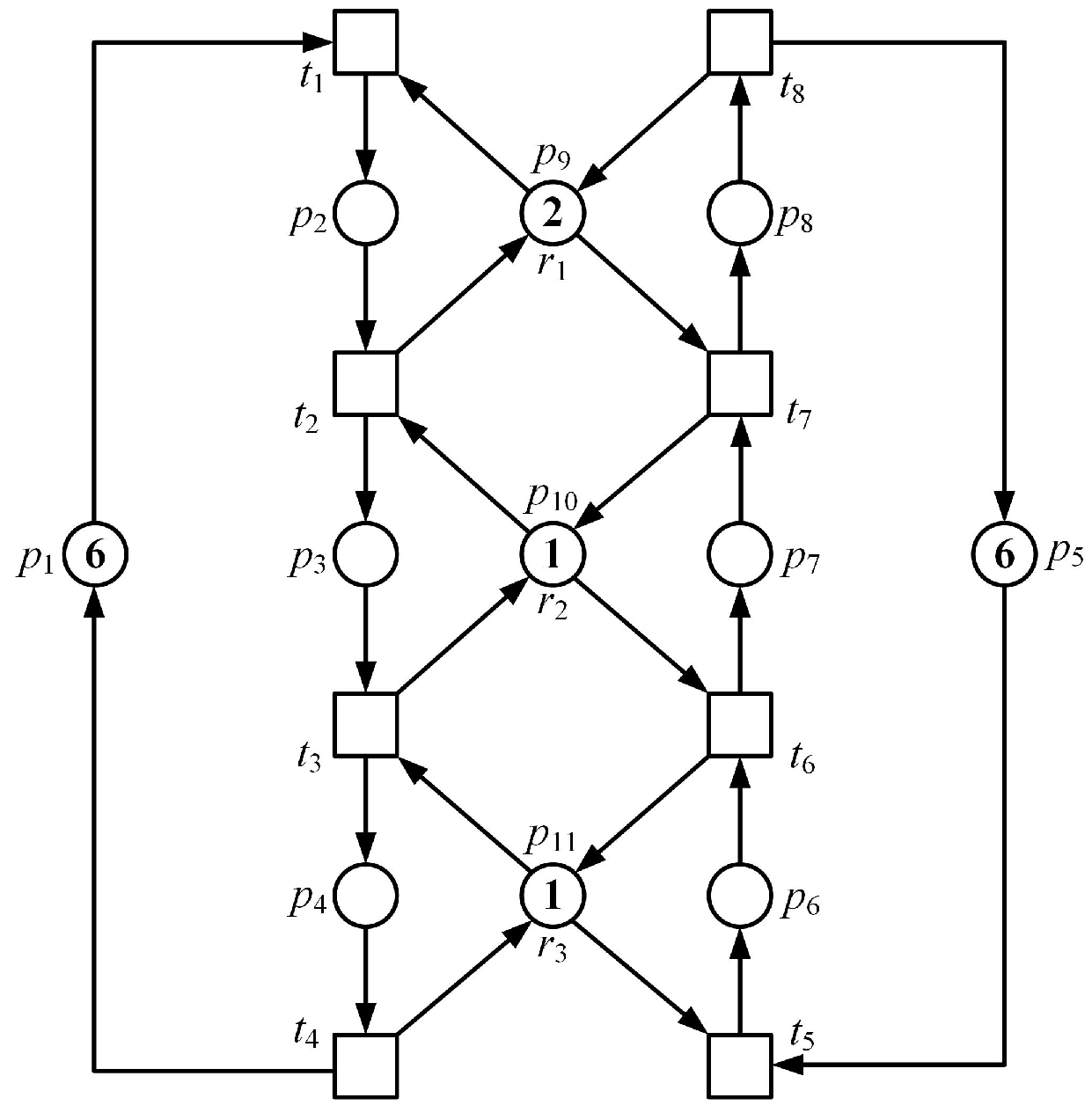
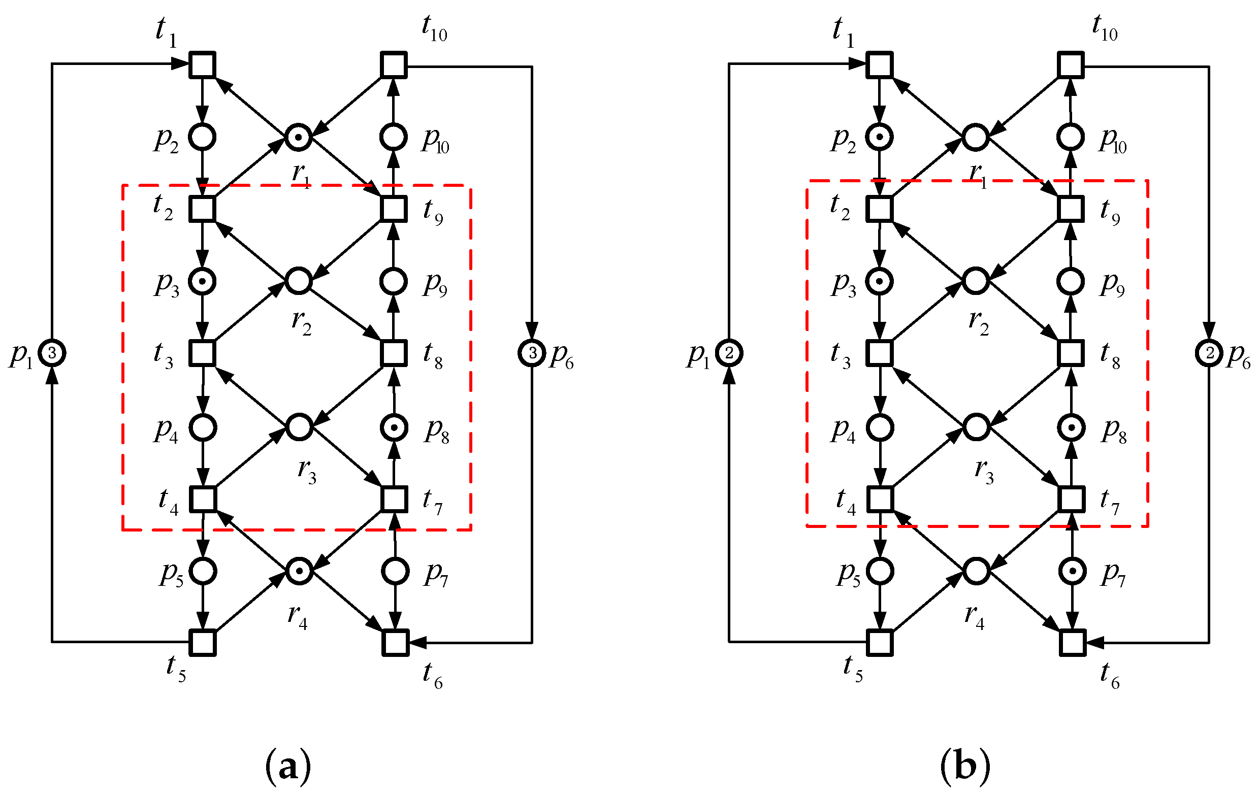
Figure 7 illustrates an ${\mathrm{S}}^3$PR net, featuring three distinct strict minimal siphons: $S_1=\{p_3,p_{10},r_1,r_2,r_4,r_5\}$, $S_2=\{p_5,p_8,r_2,r_3,r_6,r_7\}$, and $S_3=\{p_5,p_{10},r_1,r_2,r_3,r_4,r_5,r_6,r_7\}$. Two non-inclusive resource transition circuits, ${\theta }_1=r_1{t}_{11}{r}_5{t}_{10}{r}_2{t}_3{r}_4{t}_2{r}_1$ and ${\theta }_2=r_2{t}_9{r}_7{t}_8{r}_3{t}_5{r}_6{t}_4{r}_2$, are discerned.

It is noteworthy that $({\theta }_1\cap {\theta }_2)\cap P_R=\left\{r_2\right\}$, $M_0\left(r_2\right)=1$, designating $r_2$ as the exclusive $\xi$ resource in N. Furthermore, $\{r_1,r_2,r_4,r_5\}\subseteq R\left({\theta }_1\right)$ and $\{r_2,r_3,r_6,r_7\}\subseteq R\left({\theta }_2\right)$, affirming the net’s classification as a ${\mathrm{US}}^3$PR net.

Defining sets as $P^0=\left\{p_{11}\right\}\cup \left\{p_{12}\right\}$, $P_{A1}=\{p_1,p_2,p_3,p_4,p_5\}$, $P_{A2}=\{p_6,p_7,p_8,p_9,p_{10}\}$, and $P_R=\{r_1,r_2,r_4,r_5,r_6,r_7\}$, we observe a consistent pattern with $|{}^{•}{p}_i|=|{p_i}^{•}|=1$ for $i=1,2,\dots ,10$.

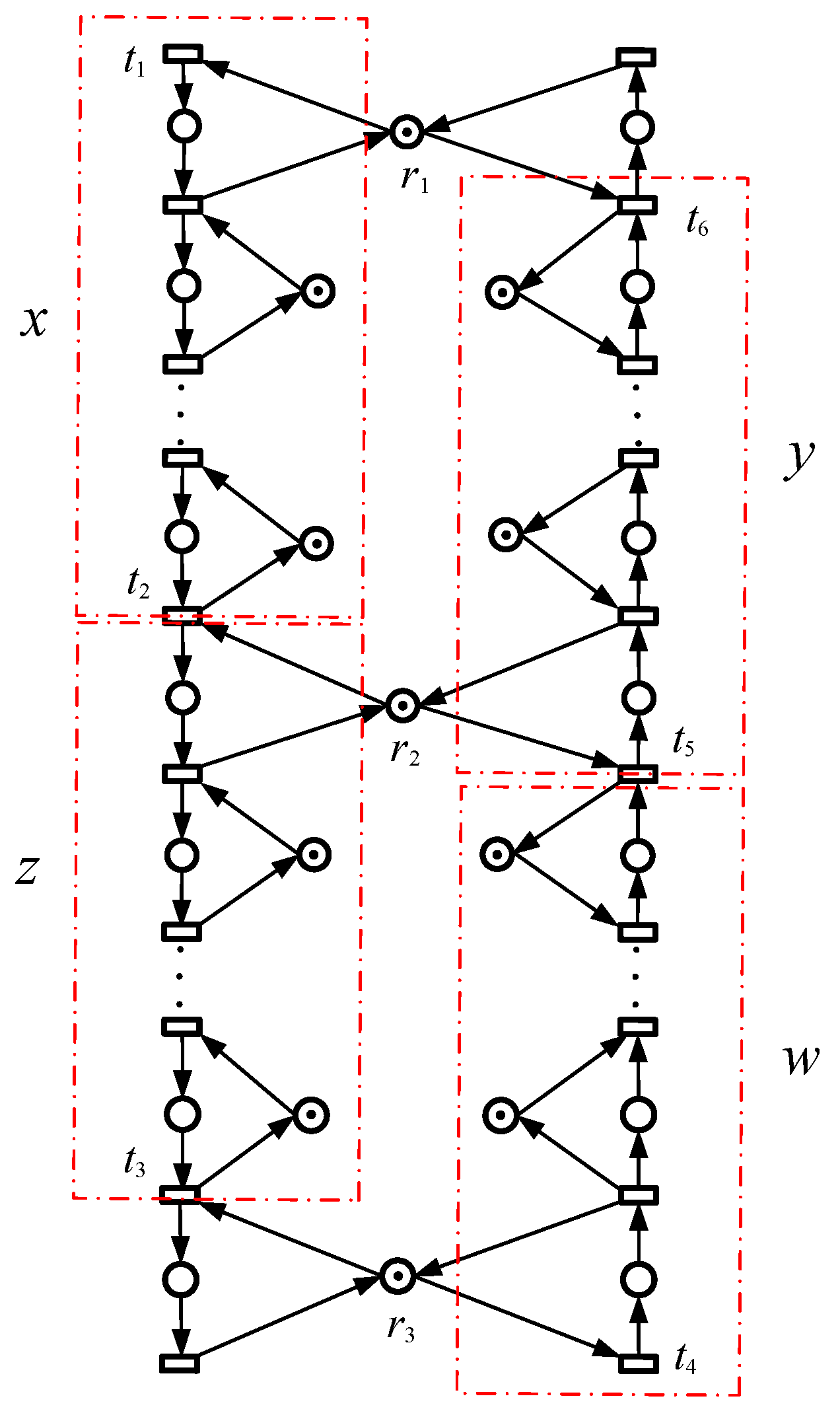
Definition 18.

Consider a dual-process ${\mathit{US}}^3$PR net denoted by $N=(P_A\cup P^0\cup P_R,T,F)$. For any $r\in P_R$, if $H\left(r\right)=\{p,p^{\prime }\}$ with $p\in P_{A1}$ and $p^{\prime }\in P_{A2}$, we designate r as a shared repository, denoted as $r_{de}$. The set of all shared repositories in N is represented by $R_{de}$.

If N is a dual-process ${\mathrm{US}}^3$PR, it must exclusively feature three shared repositories, denoted by $R_{de}=\{r_{de}^1,r_{de}^2,r_{de}^2\}$, with $r_{de}^2$ representing a $\xi$ resource place.

An RT-circuit $\theta$ necessitates a minimum of two shared resource repositories. Without this, the path formed by the resource places and transitions cannot constitute a circuit, as per Definition 17. Furthermore, as articulated in Definition 17, each process within a dual-process US3PR net lacks a branch structure. Consequently, any two adjacent shared resource repositories exclusively correspond to an RT-circuit.

Suppose there are only two shared resource repositories in N; in that scenario, only one RT-circuit $\theta$ exists, but no $\xi$ resource is present in N, leading to a contradiction with Definition 17. Conversely, assuming N contains four or more shared resource repositories would result in the formation of two or more $\xi$ resources, contradicting Definition 17. In summary, a dual-process ${\mathrm{US}}^3$PR net must invariably consist of precisely three shared resource places.

Definition 19.

If there exists a basic path $x_1,\cdots$, $x_n$, where, for all $x\in \{x_1,\cdots ,x_n\}$, $x\in P_A\cup T$, and $\{x_1,x_n\}\subseteq T$, then $x_1,\cdots ,x_n$ is considered the basic process path from $x_1$ to $x_n$, denoted as $l(x_1,x_n)$.

Definition 20.

Let $l(t_i,t_o)$ be a basic process path for the marked dual-process ${\mathit{US}}^3$PR $(N,M_0)$, and $P_{t_i-t_o}$ be the set of operation places in $l(t_i,t_o)$. If, for all $r\in R_l$, and all $p\in P_{t_i-t_o}$, there exists $r={}^{••}p\cap P_R$, then $R_l$ is referred to as a set of resource places held by $P_{t_i-t_o}$. If $M\left(P_{t_i-t_o}\right)=M_0\left(R_l\right)$, $l(t_i,t_o)$ is said to be saturated; if $M\left(P_{t_i-t_o}\right)=M_0\left(R_l\right)-1$, $l(t_i,t_o)$ is said to be progressively saturated.

Definition 21.

Let $R_{de}$ be the set of shared resources for the marked dual-process ${\mathit{US}}^3$PR $(N,M_0)$; if $r\in R_{de},r^{\prime }\in R_{de},r^{•}\cap T_1=\left\{t_r^1\right\},r^{•}\cap T_2=\left\{t_r^2\right\},{r^{\prime }}^{•}\cap T_1=\left\{t_{r^{\prime }}^1\right\}$, and ${r^{\prime }}^{•}\cap T_2=\left\{t_{r^{\prime }}^2\right\}$, then the basic process path $l(t_r^1,t_{r^{\prime }}^1)$ and $l(t_{r^{\prime }}^2,t_r^2)$ are a pair of encounter paths.

Theorem 5.

Let $l(t_r^1,t_{r^{\prime }}^1)$ and $l(t_{r^{\prime }}^2,t_r^2)$ be a pair of encounter paths in a marked dual-process ${\mathit{US}}^3$PR $(N,M_0)$; if $l(t_r^1,t_{r^{\prime }}^1)$ and $l(t_{r^{\prime }}^2,t_r^2)$ are saturated, then a deadlock occurs in N.

Proof. 

Consider a pair of encounter paths in a marked dual-process ${\mathrm{US}}^3$PR $(N,M_0)$, denoted as $l(t_r^1,t_{r^{\prime }}^1)$ and $l(t_{r^{\prime }}^2,t_r^2)$. According to Definition 21, ${}^{•}{t}_{r^{\prime }}^1\cap P_R=\left\{r^{\prime }\right\}$ and ${}^{•}{t}_r^2\cap P_R=\left\{r\right\}$, implying that firing $t_{r^{\prime }}^1$ or $t_r^2$ requires tokens in $r^{\prime }$ and r respectively.

As both $l(t_r^1,t_{r^{\prime }}^1)$ and $l(t_{r^{\prime }}^2,t_r^2)$ are saturated, the operation places in $l(t_r^1,t_{r^{\prime }}^1)$ have occupied all tokens in the associated resource places. Firing the output transition $t_{r^{\prime }}^1$ to release tokens in $r^{\prime }$ allows subsequent transitions to be fired, releasing other occupied resources. Similarly, the operation places in $l(t_{r^{\prime }}^2,t_r^2)$ have occupied all tokens in the associated resource places. Firing the output transition $t_r^2$ to release tokens in r enables subsequent transitions to release other occupied resources.

Therefore, both $l(t_r^1,t_{r^{\prime }}^1)$ and $l(t_{r^{\prime }}^2,t_r^2)$ depend on the other path to release resources first, leading to a circular wait condition. Consequently, all transitions in $l(t_r^1,t_{r^{\prime }}^1)$ and $l(t_{r^{\prime }}^2,t_r^2)$ become inactive. □

Definition 22.

In a marked dual-process ${\mathit{US}}^3$PR $(N,M_0)$, let $R_{de}=\{r_1,r_2,r_3\}$ be a set of shared resources, with $r_2$ identified as a ξ resource. Consider two pairs of encounter paths: $l(t_{r_1}^1,t_{r_2}^1)$ and $l(t_{r_2}^2,t_{r_1}^2)$, as well as $l(t_{r_2}^1,t_{r_3}^1)$ and $l(t_{r_3}^2,t_{r_2}^2)$. For any marking M in $R(N,M_0)$, M is termed a progressive encounter state if the following conditions hold: (1) $l(t_{r_1}^1,t_{r_2}^1)$ and $l(t_{r_3}^2,t_{r_2}^2)$ are saturated. (2) $l(t_{r_2}^1,t_{r_3}^1)$ and $l(t_{r_2}^2,t_{r_1}^2)$ are progressively saturated.

Theorem 6.

Given a marked dual-process ${\mathit{US}}^3$PR net $(N,M_0)$, if a progressive encounter state occurs, a deadlock occurs inevitably in N.

Proof. 

Let $l(t_{r_1}^1,t_{r_2}^1)$ and $l(t_{r_3}^2,t_{r_2}^2)$ be a pair of encounter paths of $(N,M_0)$. Referring to Definition 22, $l(t_{r_1}^1,t_{r_2}^1)$ and $l(t_{r_3}^2,t_{r_2}^2)$ are saturated, while $l(t_{r_2}^1,t_{r_3}^1)$ and $l(t_{r_2}^2,t_{r_1}^2)$ are progressively saturated. Under these circumstances, the paths have no opportunity to reach saturation, and deadlock is unlikely.

Since both $r_1$ and $r_3$ are occupied, transitions $t_{r_3}^1$ and $t_{r_1}^2$ cannot be fired, preventing a decrease in tokens in $l(t_{r_2}^1,t_{r_3}^1)$ and $l(t_{r_2}^2,t_{r_1}^2)$. The output transition of $l(t_{r_1}^1,t_{r_2}^1)$ serves as the input transition of $l(t_{r_2}^1,t_{r_3}^1)$, implying that firing $t_{r_2}^1$ would increase tokens in $l(t_{r_2}^1,t_{r_3}^1)$ and result in saturation. Similarly, firing $t_{r_2}^2$ would saturate $l(t_{r_2}^2,t_{r_1}^2)$. Given that $r_2$ is a $\xi$ resource with $M_0\left(r_2\right)=1$, simultaneous saturation of $l(t_{r_2}^1,t_{r_3}^1)$ and $l(t_{r_3}^2,t_{r_2}^2)$ is impossible. Therefore, a progressive encounter state inevitably leads to an encounter state, causing deadlocks. □

Definition 23.

Consider a dual-process ${\mathit{US}}^3$PR net $N=(P_A\cup P^0\cup P_R,T,F)$, where $R_{de}=\{r_1,r_2,r_3\}$ represents a set of shared resource places and $r_2$ is designated as the ξ resource. Let $H\left(r_2\right)=\{p_{\xi 1},p_{\xi 2}\}$. Two pairs of encounter paths corresponding to the resource pairs $r_1,r_2$ and $r_2,r_3$, are denoted as $l(t_{r_1}^1,t_{r_2}^1)$, $l(t_{r_2}^2,t_{r_1}^2)$ and $l(t_{r_2}^1,t_{r_3}^1)$, $l(t_{r_3}^2,t_{r_2}^2)$, respectively. A set of controlled places $P_L=\{P_{L1},P_{L2},P_{L3},P_{L4},P_{L5}\}\subseteq P_A$ of N is defined as follows:

• $P_{L1}=P_{t_{r_1}^1-t_{r_2}^1}\cup P_{t_{r_2}^2-t_{r_1}^2}$;
• $P_{L2}=P_{t_{r_2}^1-t_{r_3}^1}\cup P_{t_{r_3}^2-t_{r_2}^2}$;
• $P_{L3}=P_{t_{r_1}^1-t_{r_2}^1}\cup P_{t_{r_3}^2-t_{r_2}^2}\cup (P_{t_{r_2}^1-t_{r_3}^1}\setminus \left\{p_{\xi 1}\right\})\cup (P_{t_{r_2}^2-t_{r_1}^2}\setminus \left\{p_{\xi 2}\right\})$;
• $P_{L4}=P_{t_{r_1}^1-t_{r_2}^1}\cup P_{t_{r_2}^2-t_{r_3}^2}\cup (P_{t_{r_2}^1-t_{r_3}^1}\setminus \left\{p_{\xi 1}\right\})\cup (P_{t_{r_2}^2-t_{r_1}^2}\setminus \left\{p^{\prime }\right\})$, $p^{\prime }\in P_{t_{r_2}^2-t_{r_1}^2}\setminus \left\{p_{\xi 2}\right\}$;
• $P_{L5}=P_{t_{r_1}^1-t_{r_2}^1}\cup P_{t_{r_2}^2-t_{r_3}^2}\cup (P_{t_{r_2}^1-t_{r_3}^1}\setminus \left\{p^{\prime }\right\})\cup (P_{t_{r_2}^1-t_{r_3}^1}\setminus \left\{p_{\xi 2}\right\})$, $p^{\prime }\in P_{t_{r_2}^1-t_{r_3}^1}\setminus \left\{p_{\xi 1}\right\}$.

Definition 24.

Let $P_L$ denote the set of controlled places in a dual-process ${\mathit{US}}^3$PR net N. A set $R_L$ is defined as the collection of resource places held by $P_L$ if $R_L={}^{•}{P}_L\cap P_R$.

Definition 25.

Let $(N,M_0)$ be a marked dual-process ${\mathit{US}}^3$PR net, where $P_L$ is a set of controlled places of N. Add the control place $V_L$ to $(N,M_0)$, such that $g_L=P_L+V_L$ forms a P-invariant of the controlled net $(N_V,M_{0V})$, where $N_V=(P_A\cup \left\{p_0\right\}\cup P_R\cup \left\{V_L\right\},T,F\cup F_V)$, and, for all $p\in P_A\cup \left\{p^0\right\}\cup P_R$, $M_{0V}\left(p\right)=M_0\left(p\right)$, and $M_{0V}\left(V_L\right)=M_0\left(R_L\right)-1$.

Theorem 7.

Let $(N,M_0)$ be marked a dual-process ${\mathit{US}}^3$PR net; the controlled net $(N_V,M_{0V})$ defined in Definition 25 is live and maximally permissive.

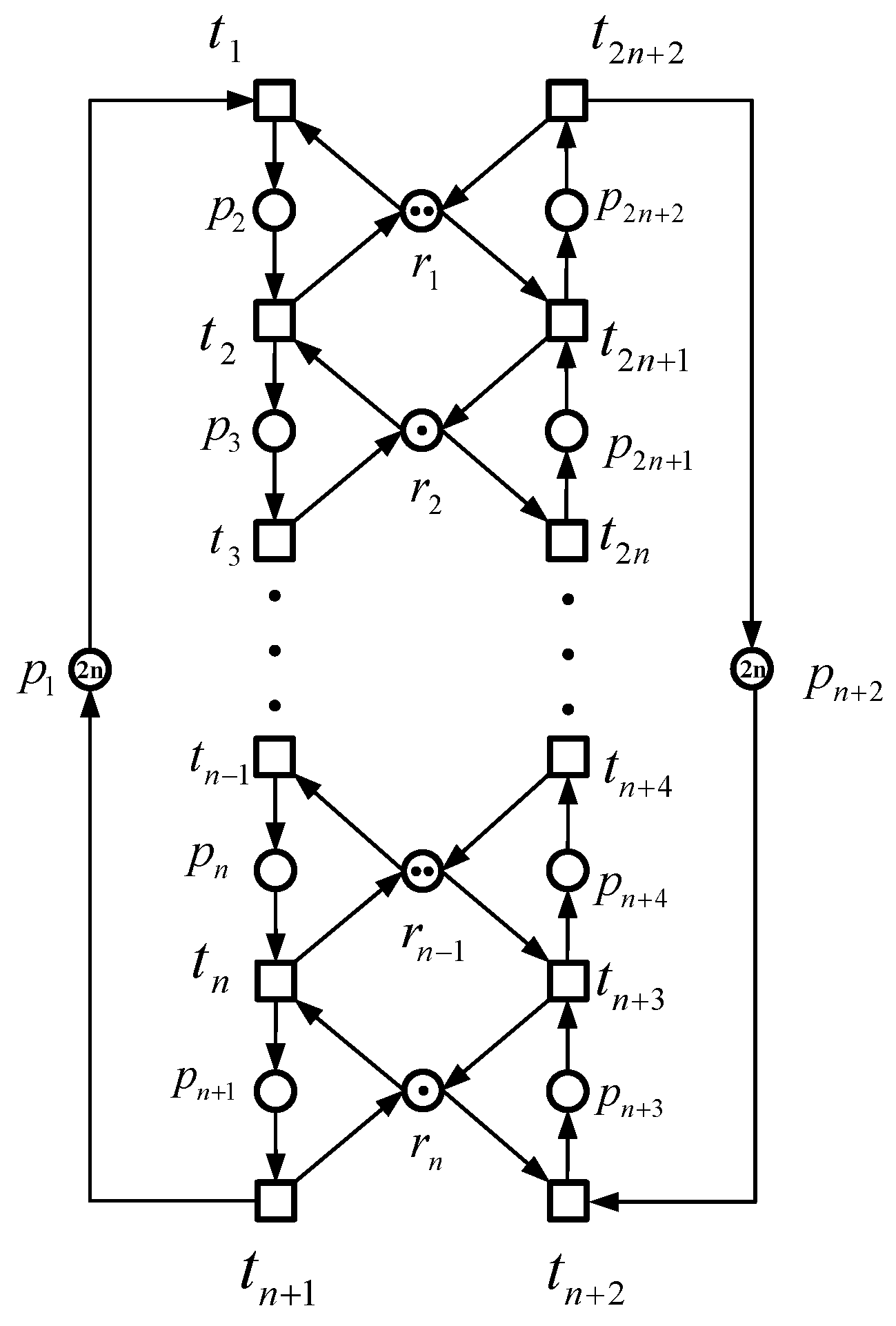
Proof. 

Given a marked dual-process ${\mathrm{US}}^3$PR net $(N,M_0)$, where the number of monoploid holder resource circuits is represented by a variable in the parameterized dual-process ${\mathrm{US}}^3$PR model, $R_{de}=\{r_1,r_2,r_3\}$ is the set of shared resource places, with $r_2$ being the $\xi$ resource, and encounter path pairs include $l(t_{r_1}^1,t_{r_2}^1)$ and $l(t_{r_2}^2,t_{r_1}^2)$ between $r_1$ and $r_2$, and $l(t_{r_2}^1,t_{r_3}^1)$ and $l(t_{r_3}^2,t_{r_2}^2)$ between $r_2$ and $r_3$. Let x, y, z, and w represent the number of operation places in $(t_{r_1}^1,t_{r_2}^1)$, $l(t_{r_2}^2,t_{r_1}^2)$, $l(t_{r_2}^1,t_{r_3}^1)$, and $l(t_{r_3}^2,t_{r_2}^2)$, respectively, where $x,y,z,w\in {\mathbb{N}}^{+}$.

According to Definition 25, control places are added to $(N,M_0)$ to obtain the controlled net $(N_V,M_{0V})$. Since the control places and the controlled place set form a P-invariant of $(N_V,M_{0V})$, where $M_{0V}\left(V_L\right)=M_0\left(R_L\right)-1$, and the encounter path pair $l(t_{r_1}^1,t_{r_2}^1)$ and $l(t_{r_2}^2,t_{r_1}^2)$ satisfies the condition that, for all $M\in R(N,M_0)$, $M\left(P_{t_{r_1}^1-t_{r_2}^1}\right)+M\left(P_{t_{r_2}^2-t_{r_1}^2}\right)\le M_0\left(R_L\right)-1$, the encounter path pair $l(t_{r_1}^1,t_{r_2}^1)$ and $l(t_{r_2}^2,t_{r_1}^2)$ will not saturate. Consequently, no deadlock is generated, and the workpiece in x can enter z by firing $t_{r_2}^1$, and the workpiece in y can be exported by firing $t_{r_1}^2$. Similarly, for the encounter path pair $l(t_{r_2}^1,t_{r_3}^1)$ and $l(t_{r_3}^2,t_{r_2}^2)$, after adding the control place, ensuring that the workpiece in w can enter y by firing $t_{r_2}^2$, the workpiece in z can be exported by firing $t_{r_3}^1$. The controlled net $(N_V,M_{0V})$ is live.

The initial marking of control place $M_{0V}\left(V_L\right)=M_0\left(R_L\right)-1$. Compared to the original net $(N,M_0)$, the controlled net $(N_V,M_{0V})$ only eliminates the encounter state and the progressive encounter state in the reachable graph, retaining all states except these two special states. As the encounter state and the progressive encounter state can cause deadlock or inevitably lead to deadlock, they correspond to the dead states and bad states in the reachable graph of $(N,M_0)$. The controlled net removes only the dead states and bad states compared to the original net while retaining all legal states. Therefore, $(N_V,M_{0V})$ is maximally permissive. □

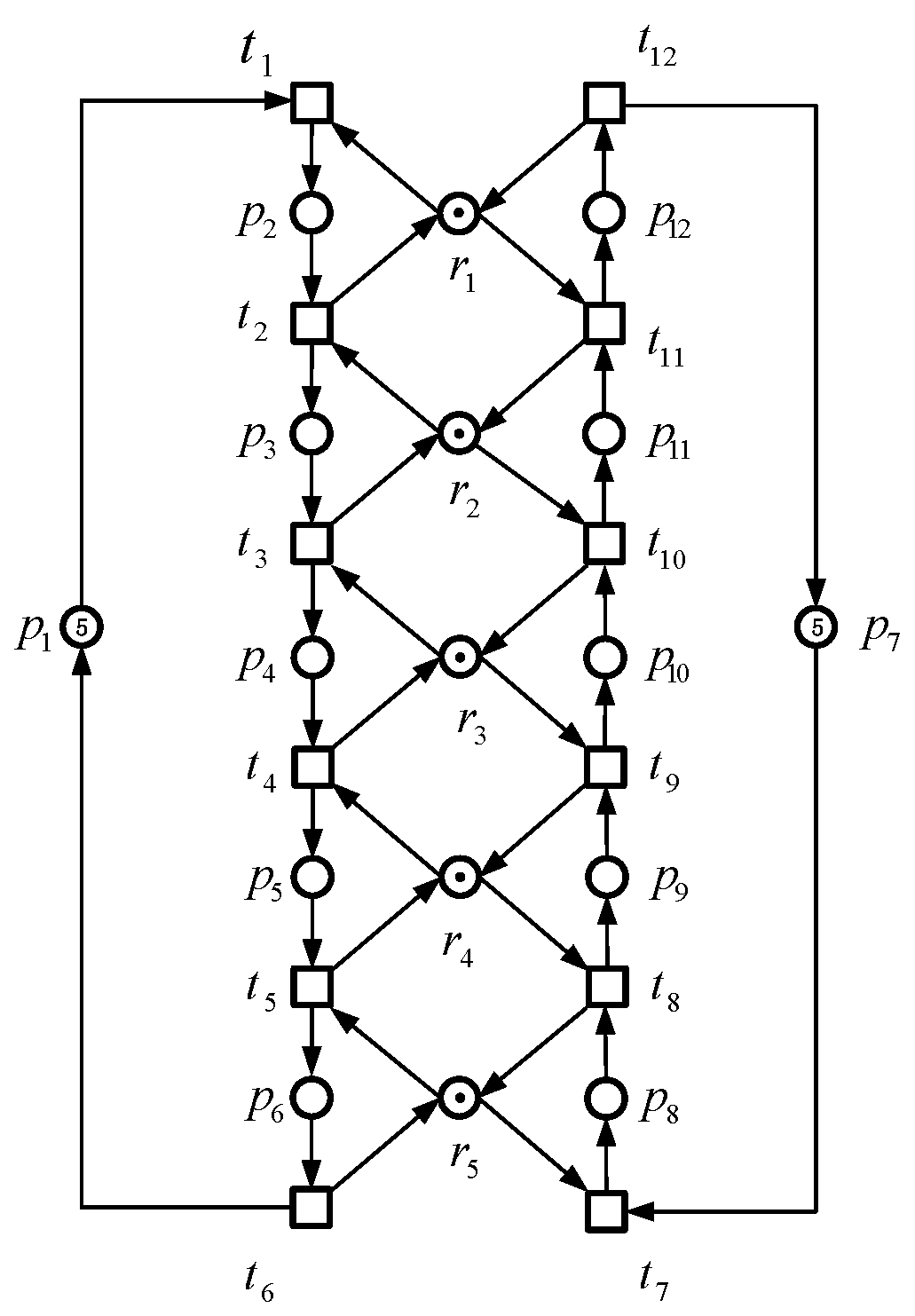
Figure 8 shows a dual-process ${\mathrm{US}}^3$PR net $(N,M_0)$, where $R_{de}=\{r_1,r_2,r_3\}$, $t_{r_1}^1=t_1$, $t_{r_2}^1=t_2$, $t_{r_3}^1=t_3$, $t_{r_3}^2=t_4$, $t_{r_2}^2=t_5$, $t_{r_1}^2=t_6$, the number of operation places in $l(t_1,t_2)$, $l(t_5,t_6)$, $l(t_2,t_3)$, and $l(t_4,t_5)$ are x, y, z, and w, respectively.

Theorem 8.

Let $(N,M_0)$ be a marked dual-process ${\mathit{US}}^3$PR, and x, y, z, and w respectively represents the number of operation places in $(t_{r_1}^1,t_{r_2}^1)$, $l(t_{r_2}^2,t_{r_1}^2)$, $l(t_{r_2}^1,t_{r_3}^1)$, and $l(t_{r_3}^2,t_{r_2}^2)$, where $V_L$ is the number of control places added according to Definition 25. As a result, k is only related to y and z, and satisfies $k=1+y+z$.

Proof. 

The control places $V_L$ defined by Definition 25 have a one-to-one correspondence with $P_L$. Therefore, the number k of $V_L$ is equal to the number $k^{\prime }$ of $P_L$. According to Definition 23, the following conditions are satisfied:

(1) The controlled place set is the set of operation places in the encounter path pair $l(t_{r_1}^1,t_{r_2}^1)$ and $l(t_{r_2}^2,t_{r_1}^2)$, denoted as $P_L^1=P_{t_{r_1}^1-t_{r_2}^1}\cup P_{t_{r_2}^2-t_{r_1}^2}$.

(2) The controlled place set is the set of operation places in the encounter path pair $l(t_{r_2}^1,t_{r_3}^1)$ and $l(t_{r_3}^2,t_{r_2}^2)$, denoted as $P_L^2=P_{t_{r_2}^1-t_{r_3}^1}\cup P_{t_{r_3}^2-t_{r_2}^2}$.

(3) The controlled place set is the set of operation places in the encounter path pair $l(t_{r_1}^1,t_{r_2}^1)$ and $l(t_{r_2}^2,t_{r_1}^2)$, $l(t_{r_2}^1,t_{r_3}^1)$ and $l(t_{r_3}^2,t_{r_2}^2)$, which excludes the set of places in $H\left(r_2\right)=\{p_{\xi 1},p_{\xi 2}\}$, i.e., $P_L^3=P_{t_{r_1}^1-t_{r_2}^1}\cup P_{t_{r_3}^2-t_{r_2}^2}\cup (P_{t_{r_2}^1-t_{r_3}^1}\setminus \left\{p_{\xi 1}\right\})\cup (P_{t_{r_2}^2-t_{r_1}^2}\setminus \left\{p_{\xi 2}\right\})$.

(4) If $p^{\prime }\in P_{t_{r_2}^2-t_{r_1}^2}\setminus \left\{p_{\xi 2}\right\}=P_{t_{r_2}^2-t_{r_1}^2}\setminus \left\{p_{\xi 2}\right\}$, where $P_{t_{r_2}^2-t_{r_1}^2}$ contains y operation places, the number of $p^{\prime }$ is $y-1$. Correspondingly, the number of $P_L$ is $y-1$. Similarly, if $p^{\prime }\in P_{t_{r_2}^1-t_{r_3}^1}\setminus \left\{p_{\xi 1}\right\}=P_{t_{r_2}^1-t_{r_3}^1}\setminus \left\{p_{\xi 1}\right\}$, the number of $P_L$ is $z-1$. In summary, the number of $P_L$ is $k^{\prime }=1+1+1+(y-1)+(z-1)=1+y+z$, and the number of $V_L$, i.e., $k=k^{\prime }=1+y+z$. □

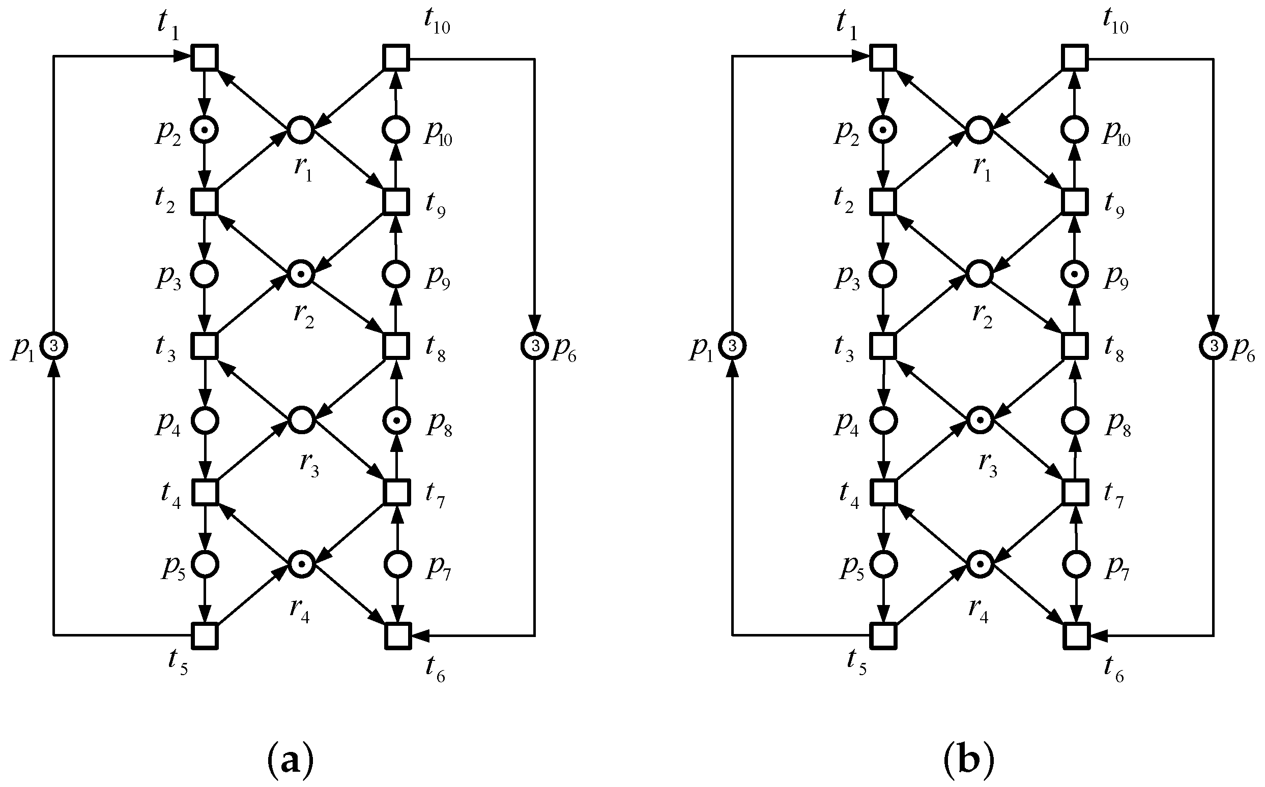
Example 2.

In the dual-process ${\mathit{US}}^3$PR net shown in Figure 7, since the number of reachable states is 405, and the number of good states is 380, the net is dead. The sets $P_L$ and $R_L$ are presented in

Table 4. $P_L$ and $R_L$ of the dual-process ${\mathrm{US}}^3$PR shown in Figure 7.

	${\mathit{P}}_{\mathit{L}}$	${\mathit{R}}_{\mathit{L}}$
1	$p_1,p_2,p_8,p_9$	$r_1,r_2,r_4,r_5$
2	$p_3,p_4,p_6,p_7$	$r_2,r_3,r_6,r_7$
3	$p_1,p_2,p_4,p_6,p_7,p_9$	$r_1,r_3,r_4,r_5,r_6,r_7$
4	$p_1,p_2,p_4,p_6,p_7,p_8$	$r_1,r_2,r_3,r_4,r_6,r_7$
5	$p_1,p_2,p_3,p_6,p_7,p_9$	$r_1,r_2,r_3,r_4,r_5,r_7$

. According to Definition 25, a control place needs to be added to each controlled place set. The control places and the controlled place set together form a P-invariant, and the control places are listed in

Table 5. The control places of the dual-process ${\mathrm{US}}^3$PR shown in Figure 7.

${\mathit{P}}_{\mathit{V}}$	${\mathit{M}}_0\left(\mathit{V}\right)$	${}^{•}\mathit{V}$	${\mathit{V}}^{•}$
$V_L^1$	3	$t_3,t_{11}$	$t_1,t_9$
$V_L^2$	3	$t_5,t_9$	$t_3,t_7$
$V_L^3$	5	$t_3,t_5,t_9,t_{11}$	$t_1,t_4,t_7,t_{10}$
$V_L^4$	5	$t_4,t_9,t_{11}$	$t_1,t_7,t_{10}$
$V_L^5$	5	$t_3,t_5,t_{10}$	$t_1,t_4,t_7$

. As a result, the controlled net $(N_V,M_{0V})$ with 380 reachable states is live and maximally permissive.

5. Conclusions

In this paper, two special subclasses in the ${\mathrm{S}}^3$PR are studied: the dual-process ${\mathrm{S}}^3$PR and the dual-process ${\mathrm{US}}^3$PR network models. By analyzing the relationship between their structural characteristics and deadlocks, some control laws are proposed, avoiding complicated calculations. In the future, we plan to research control laws for a more universal dual-process ${\mathrm{S}}^3$PR model that does not limit the initial marking of resource places to 1.

For the convenience of analysis, each process in the dual-process ${\mathrm{S}}^3$PR and the dual-process ${\mathrm{US}}^3$PR is defined without a branch structure, making the model relatively simple. Therefore, extending the model to include multiple processes or multiple branches in each process, and then conducting control law research, is also the focus of the next step.